Centrality bin size dependence of multiplicity correlation
in central Au+Au collisions at $\sqrt{s_{\rm{NN}}}$=200 GeV

Abstract

We have studied the centrality bin size dependence of charged particle forward-backward multiplicity correlation strength in 5%, 0-5%, and 0-10% most central Au+Au collisions at $\sqrt{s_{\rm{NN}}}$=200 GeV with a parton and hadron cascade model, PACIAE based on PYTHIA. The real (total), statistical, and NBD (Negative Binomial Distribution) correlation strengths are calculated by the real events, the mixed events, and fitting the charged particle multiplicity distribution to the NBD, respectively. It is turned out that the correlation strength increases with increasing centrality bin size monotonously. If the discrepancy between real (total) and statistical correlation strengths is identified as dynamical one, the dynamical correlation may just be a few percent of the total (real) correlation.

I INTRODUCTION

The study of fluctuations and correlations has been suggested as a useful means for revealing the mechanism of particle production and Quark-Gluon-Plasma (QGP) formation in Relativistic Heavy Ion Collisions hwa2 ; naya . Correlations and fluctuations of the thermodynamic quantities and/or the produced particle distributions may be significantly altered when the system undergoes phase transition from hadronic matter to quark-gluon matter because the degrees of freedom in two matters is very different.

The experimental study of fluctuations and correlations becomes a hot topic in relativistic heavy ion collisions with the availability of high multiplicity event-by-event measurements at the CERN-SPS and BNL-RHIC experiments. An abundant experimental data have been reported star2 ; phen2 ; phob where a lot of new physics arise and are urgent to be studied. A lot of theoretical investigations have been reported as well paja ; hwa1 ; konc ; brog ; fu ; yan ; bzda .

Recently STAR collaboration have measured the charged particle forward-backward multiplicity correlation strength $b$ in Au+Au collisions at $\sqrt{s_{\rm{NN}}}$=200 GeV star3 ; star4 . The outstanding features of STAR data are:

• In most central collisions, the correlation strength $b$ is approximately flat across a wide range in $\Delta\eta$ which is the distance between the centers of forward and backward (pseudo)rapidity bins.

• This trend disappears slowly with decreasing centrality and approaches a exponential function of $\Delta\eta$ at the peripheral collisions.

That has stimulated a lot of theoretical interests konc ; brog ; fu ; bzda .

In Ref. fu , a statistical model was proposed to calculate the charged particle forward-backward multiplicity correlation strength $b$ in 0-10% most central Au+Au collisions at $\sqrt{s_{\rm{NN}}}$=200 GeV. One outstanding feature of STAR data, the $b$ as a function of $\Delta\eta$ is approximately flat, was well reproduced. The calculated value of $b\approx 0.44$ was compared with STAR data of $b\approx 0.60$ star3 ; star4 .

However, in this statistical model fu the Negative Binomial Distribution (NBD) is assumed for the charged multiplicity distribution and the NBD parameters of $\mu$ and $k$ (see later) are extracted from fit in with PHENIX charged particle multiplicity distribution phen3 . It is turned out in Ref. yan that the experimental $\eta$ and $p_{T}$ acceptances have large influences on the correlation strength $b$. The STAR experimental acceptances are quite different from PHENIX, thus the inconsistency, using PHENIX multiplicity data to explain STAR correlation data, involved in fu have to be studies further. Meanwhile, what is the discrepancy between $b\approx 0.60$ (STAR datum) and $b\approx 0.44$ (NBD) also needs to be answered.

In this paper we use a parton and hadron cascade model PACIAE sa , to investigate the centrality bin size dependence of charged particle multiplicity correlation in 5, 0-5, and 0-10% most central Au+Au collisions at $\sqrt{s_{\rm{NN}}}$=200 GeV. Following Ref. yan we generate the real events (6000) by the PACIAE model, construct the mixed events according to real events one by one, and extract the NBD parameters ($\mu$ and $k$) from fitting the real events charged particle multiplicity distribution to the NBD. Then the charged particle forward-backward multiplicity correlation strength $b$ is calculated for the real events (real correlation strength), the mixed events (statistical correlation strength), and the NBD (NBD correlation strength), respectively. They are all nearly flat across a widw range in $\Delta\eta$. Their magnitude in 0-10% most central Au+Au collisions are about 0.63, 0.59, and 0.52, respectively. So the corresponding STAR data is well reproduced. It is turned out that the real (total), statistical, and NBD correlation strengths increase with increasing centrality bin size monotonously. If the discrepancy between real (total) and statistical correlation strengths is identified as dynamical one, then the dynamical correlation strength may just be a few percent of the total (real) correlation strength.

II PACIAE MODEL

The parton and hadron cascade model, PACIAE sa , is based on PYTHIA soj2 which is a model for hadron-hadron ($hh$) collisions. The PACIAE model is composed of four stages: parton initialization, parton evolution (rescattering), hadronization, and hadron evolution (rescattering).

II.1 Parton initialization

In the PACIAE model a nucleon-nucleon ($NN$) collision is described with PYTHIA model, where a $NN$ ($hh$) collision is decomposed into the parton-parton collisions. The hard parton-parton collision is described by the lowest-leading-order (LO) pQCD parton-parton cross section comb with modification of parton distribution function in the nucleon. And the soft parton-parton interaction is considered empirically. The semihard, between hard and soft, QCD $2\rightarrow 2$ processes are also involved in PYTHIA (PACIAE) model. Because of the initial- and final-state QCD radiation added to the above processes, the PYTHIA (PACIAE) model generates a multijet event for a $NN$ ($hh$) collision. That is followed, in the PYTHIA model, by the string-based fragmentation scheme (Lund model and/or Independent Fragmentation model), thus a hadronic state is reached for a $NN$ ($hh$) collision. However, in the PACIAE model above string fragmentation is switched off temporarily, so the result is a multijet event (composed of quark pairs, diquark pairs and gluons) instead of a hadronic state. If the diquarks (anti-diquarks) are split forcibly into quarks (anti-quarks) randomly, the consequence of a $NN$ ($hh$) collision is its initial partonic state composed of quarks, anti-quarks, and gluons.

A nucleus-nucleus collision, in the PACIAE model, is decomposed into the nucleon-nucleon collisions based on the collision geometry. A nucleon in the colliding nucleus is randomly distributed in the spatial coordinate space according to the Woods-Saxon distribution ($r$) and the 4$\pi$ uniform distribution ($\theta$ and $\phi$). The beam momentum is given to $p_{z}$ and $p_{x}=p_{y}=0$ is assumed for each nucleon in the colliding nucleus. A closest approaching distance of two assumed straight line trajectories is calculated for each $NN$ pair. If this distance is less than or equal to $\displaystyle{\sqrt{\sigma_{\rm{tot}}/\pi}}$, then it is considered as a collision pair. Here $\sigma_{\rm{tot}}$ refers to the total cross section of $NN$ collision assumed to be 40 mb. The corresponding collision time of this collision pair is then calculated. So the particle list and the $NN$ collision (time) list can be constructed. A $NN$ collision pair with smallest collision time is selected from the $NN$ collision (time ) list and performed by the method in former paragraph. After upgrading the particle list and collision (time) list we select and perform a new $NN$ collision pair again. Repeat these processes until the collision (time) list is empty we obtain a initial partonic state for a nucleus-nucleus collision.

II.2 Parton evolution (rescattering)

The next step, in the PACIAE model, is parton evolution (partonic rescattering). Here the $2\rightarrow 2$ LO-pQCD differential cross sections comb are employed. The differential cross section for a subprocess $ij\rightarrow kl$ reads

$$\frac{d\sigma_{ij\rightarrow kl}}{d\hat{t}}=K\frac{\pi\alpha_{s}^{2}}{\hat{s}}\sum_{ij\rightarrow kl},$$ (1)

where the $K$ factor is introduced for higher order corrections and the non-perturbative QCD correction as usual. Take the process $q_{1}q_{2}\rightarrow q_{1}q_{2}$ as an example, one has

$$\sum_{q_{1}q_{2}\rightarrow q_{1}q_{2}}=\frac{4}{9}\frac{\hat{s}^{2}+\hat{u}^{2}}{\hat{t}^{2}},$$ (2)

which can be regularized as

$$\sum_{q_{1}q_{2}\rightarrow q_{1}q_{2}}=\frac{4}{9}\frac{\hat{s}^{2}+\hat{u}^{2}}{(\hat{t}-m^{2})^{2}}$$ (3)

by introducing the parton colour screen mass, $m$=0.63 GeV. In above equation $\hat{s}$, $\hat{t}$, and $\hat{u}$ are the Mandelstam variables and $\alpha_{s}$= 0.47 stands for the running coupling constant. The total cross section of the parton collision $i+j$ is

$$\sigma_{ij}(\hat{s})=\sum_{k,l}\int_{-\hat{s}}^{0}d\hat{t}\frac{d\sigma_{ij\to kl}}{d\hat{t}}.$$ (4)

With these total and differential cross sections the parton evolution (rescattering) can be simulated by the Monte Carlo method until the parton-parton collision is ceased (partonic freeze-out).

II.3 Hadronization

In the PACIAE model the partons can be hadronized with the string-based fragmentation scheme or by the coalescence (recombination) models biro ; csiz ; grec ; hwo ; frie . The Lund string fragmentation regime, involved in the PYTHIA model, is adopted for hadronization in this paper, see soj2 for the details.

Meanwhile, we have proposed a simulant coalescence (recombination) model which can be briefly explained as follows:

1. The Field-Feynman parton generation mechanism ff1 is first applied to deexcite the energetic parton and thus to increase the parton multiplicity. This deexcitation of an energetic parton plays a similar role as string multiple fragmentation in the Lund model and1 .

2. The gluons are forcibly split into $q\bar{q}$ pair randomly.

3. In the program there is a hadron table composed of mesons and baryons. The pseudoscalar and vector mesons made of u, d, s, and c quarks, as well as $B^{+}$, $B^{0}$, $B^{*0}$, and $\Upsilon$ are considered. The SU(4) multiplets of baryons made of u, d, s, and c quarks (except those with double c quarks) as well as $\Lambda^{0}_{b}$ are considered.

4. Two partons can coalesce into a meson and three partons into a baryon (antibaryon) according to the flavor, momentum, and spatial coordinates of partons and the valence quark structure of hadron.

5. When the coalescing partons can form either a pseudoscalar meson or a vector meson (e. g. $u\bar{d}$ can form either a $\pi^{+}$ or a $\rho^{+}$) a judgment of less discrepancy between the invariant mass of coalescing partons and the mass of coalesced hadron is invoked to select one from two mesons above. In the case of baryon, e. g. both $p$ and $\Delta^{+}$ are composed of $uud$, the same judgment is invoked to select one baryon from both of $\frac{1}{2}^{+}$ and $\frac{3}{2}^{+}$ baryons.

6. Four momentum conservation is required.

7. There is a phase space condition

   $$\frac{16\pi^{2}}{9}\Delta r^{3}\Delta p^{3}=\frac{h^{3}}{d},$$ (5)

   where $h^{3}/d$ is the volume occupied by a single hadron in the phase space, $d$=4 refers to the spin and parity degeneracies, $\Delta r$ and $\Delta p$ stand for the spatial and momentum distances between coalescing partons, respectively.

II.4 Hadron evolution (rescattering)

We obtain a configuration of hadrons in spatial and momentum coordinate spaces for a nucleus-nucleus collision after the hadronization. If one only considers the rescattering among $\pi,k,p,n,\rho(\omega),\Delta,\Lambda,\Sigma,\Xi,\Omega,J/\Psi$ and their antiparticles, the particle list is then constructed by the above hadrons. A closest approaching distance of two assumed straight line trajectories is calculated for each $hh$ pair. If this distance is less than or equal to $\displaystyle{\sqrt{\sigma_{\rm{tot}}^{hh}/\pi}}$ sa1 , then it is considered as a collision pair. Here $\sigma_{\rm{tot}}^{hh}$ refers to the total cross section of $hh$ collision. The corresponding collision time of this collision pair is then calculated. So the $hh$ collision (time) list can be constructed. A $hh$ collision pair with smallest collision time is selected from the collision (time) list and performed by the usual two-body collision method sa1 . After upgrading the particle list and collision (time) list we select and perform a new $hh$ collision pair again. Repeat these processes until the collision (time) list is empty (hadronic freeze-out).

A isospin averaged parametrization formula is used for the $hh$ cross section koch ; bald . However, we also provide a option of constant total, elastic, and inelastic cross sections sa1 : $\sigma_{\rm{tot}}^{NN}=40$ mb, $\sigma_{\rm{tot}}^{\pi N}=25$ mb, $\sigma_{\rm{tot}}^{kN}=35$ mb, $\sigma_{\rm{tot}}^{\pi\pi}=10$ mb, and the assumed ratio of inelastic to total cross section equals 0.85. We also assume

$$\sigma_{pp}=\sigma_{pn}=\sigma_{nn}=\sigma{\Delta N}=\sigma{\Delta\Delta}.$$ (6)

The cross section of $\pi\bar{N}$ and $k\bar{N}$, for instance, is assumed to be equal to the cross section of $\pi N$ and $kN$, respectively.

The momentum of scattered particles in a $hh$ elastic collision is simulated according to that the $hh$ differential cross section, $d\sigma_{\rm{tot}}^{hh}/dt$, is assumed to be an exponential function of $t$ which is squared momentum transfer sa1 . As it is impossible to include all inelastic channels, we consider only a part of them ($\approx$ 600) which have noticeable effects on the hadronic final state, and the rest is attributed to the elastic scattering. Take incident channel $\pi N$ as an example, if there are possible final channels of $\pi N\rightarrow\pi\Delta$, $\pi N\rightarrow\rho N$, and $\pi N\rightarrow k\Lambda$, their relative probabilities are then used to select one among above three channels. The momentum of scattered particles in a $hh$ inelastic collision is simulated according to the usual two-body kinematics sa1 ; pdg .

III CALCULATION AND RESULT

Following cape the charged particle forward-backward multiplicity correlation strength $b$ is defined as

$$\ b=\frac{\langle n_{f}n_{b}\rangle-\langle n_{f}\rangle\langle n_{b}\rangle}{\langle n_{f}^{2}\rangle-\langle n_{f}\rangle^{2}}=\frac{{\rm{cov}}(n_{f},n_{b})}{{\rm{var}}(n_{f})},$$ (7)

where $n_{f}$ and $n_{b}$ are, respectively, the number of charged particles in forward and backward pseudorapidity bins defined relatively and symmetrically to a given pseudorapidity $\eta$. $\langle n_{f}\rangle$ refers to the mean value of $n_{f}$ for instance. cov($n_{f}$,$n_{b}$) and var($n_{f}$) are the forward-backward multiplicity covariance and forward multiplicity variance, respectively.

Table 1: Total charged particle multiplicity in three $\eta$ fiducial ranges in 0-6% most central Au+Au collisions at $\sqrt{s_{\rm{NN}}}$=200 GeV.

	$N_{\rm{ch}}(|\eta|<4.7)$	$N_{\rm{ch}}(|\eta|<5.4)$	$N_{\rm{ch}}$(total)
PHOBOSa	4810 $\pm$ 240	4960 $\pm$ 250	5060 $\pm$ 250
PACIAE	4819	4983	5100
a The experimental data are taken from phob2 .

In the calculations the default values given in the PYTHIA model are adopted for all model parameters except the parameters $K$ and $b_{s}$ (in the Lund string fragmentation function). The $K$=3 is assumed and the $b_{s}$=6 is fixed by fitting the charged particle multiplicity to the corresponding PHOBOS data in 0-6% most central Au+Au collisions at $\sqrt{s_{\rm{NN}}}$=200 GeV phob2 as shown in Tab. 1. Therefore in the generation of real events there is no free parameters. The mapping relation sa2 between the centrality definition in theory and experiment

$$b_{i}=\sqrt{g}b_{i}^{\rm{max}},\qquad b_{i}^{\rm{max}}=R_{A}+R_{B},$$ (8)

is employed. In the above equation $b_{i}$ (in fm) refers to the theoretical impact parameter and $g$ stands for the percentage of geometrical (total) cross section used in experiment to define the centrality. $R_{A}=1.12A^{1/3}+0.45$ fm, for instance, is the radius of nucleus $A$. Thus the 0-10, 0-6, 0-5, and 5% most central collisions, for instance, are mapped to $0<b_{i}<4.46$, $0<b_{i}<3.53$, $0<b_{i}<3.20$, and $b_{i}=3.20$ fm, respectively.

In this paper we propose a mixed event method where the mixed events are generated according to real events one by one. We first assume the charged particle multiplicity $n$ in a mixed event is the same as one corresponding real event. However, $n$ particles of this mixed event are sampled randomly from the particle reservoir composed of all particles in all real events. Therefore, there is no dynamical relevance among the particles in a mixed event. So the correlation calculated by mixed events is reasonably to be identified as the statistical correlation yan .

It is known that the statistical correlation can also be studied by the NBD method, because the charged particle multiplicity distribution in high energy heavy-ion collisions is close to NBD phen3 . For an integer $n$ the NBD reads

$$\ P(n;\mu,k)=\begin{pmatrix}n+k-1\\ k-1\end{pmatrix}\frac{(\mu/k)^{n}}{(1+\mu/k)^{n+k}},$$ (9)

where $\mu\equiv\langle n\rangle$ is a parameter, $P(n;\mu,k)$ is normalized in $0\leq n\leq\infty$, and $k$ is another parameter responsible for the shape of the distribution. As proved in yan the correlation strength can be expressed as

$$\ b=\frac{\langle n_{f}\rangle}{\langle n_{f}\rangle+k},$$ (10)

where the parameter $k$ is fixed by fitting the charged particle multiplicity to the NBD usually.

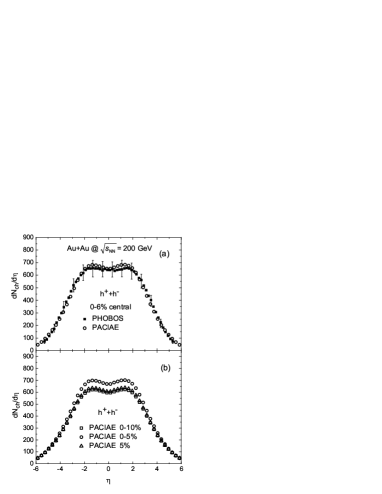
Figure 1: Charged particle pseudorapidity distribution in Au+Au collision at $\sqrt{s_{\rm{NN}}}$=200 GeV: (a) 0-6% most central collision and (b) 0-10, 0-5, and 5% most central collision. The experimental data are taken from phob2 .

We compare the theoretical charged particle pseudorapidity distribution (open circles) in 0-6% most central Au+Au collisions at $\sqrt{s_{\rm{NN}}}$=200 GeV with the corresponding PHOBOS data (solid squares) phob2 in Fig. 1 (a). One sees here that the PHOBOS data are well reproduced. In Fig. 1 (b), we compare the charged particle pseudorapidity distributions in 0-5% (open circles) and 5% (open triangles) most central Au+Au collisions with the 0-10% one (open squares). We see in Fig. 1 (b) that the pseudorapidity distribution in 5% most central collision is quite close to the 0-10% one, because the 5% centrality is nearly equal to the average centrality of 0-10% centrality bin.

Figure 2: Charged particle forward-backward multiplicity correlation strength $b$ in 0-10, 0-5, and 5% most central Au+Au collisions at $\sqrt{s_{\rm{NN}}}$=200 GeV. The experimental data are taken from star3 .

In Fig. 2 we compare the calculated real (total) correlation strength $b$ (open squares) as a function of $\Delta\eta$ in 0-10% most central Au+Au collisions at $\sqrt{s_{\rm{NN}}}$=200 GeV with the corresponding STAR data (solid squares) star3 . The STAR data feature of correlation strength $b$ is approximately flat across a wide range in $\Delta\eta$ are well reproduced. For comparison we also give the real (total) correlation strength in 0-5 and 5% most central collisions by open circles and triangles, respectively. One sees here that the real (total) correlation strength decreases with decreasing centrality bin size monotonously, because the charged particle multiplicity fluctuation decreases from 0-10 to 0-5 and to 5% monotonously, as one will see in Fig. 3. This first result of the correlation strength increases with increasing centrality bin size monotonously given in the transport model remains to be proved experimentally.

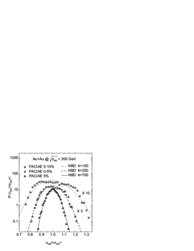
Figure 3: Charged particle multiplicity distributions in 0-10 (open squares), 0-5 (open circles), and 5% (open triangles) most central Au+Au collisions at $\sqrt{s_{\rm{NN}}}$=200 GeV. The dotted, dashed, and solid lines are the corresponding NBD fits, respectively.

The calculated charged particle multiplicity distributions in 0-10, 0-5, and 5% most central Au+Au collisions at $\sqrt{s_{\rm{NN}}}$=200 GeV are given in Fig. 3, respectively, by the open squares, circles and triangles. The corresponding NBD fits are shown by dotted, dashed, and solid lines, respectively. One sees in Fig. 3 that the charged particle multiplicity fluctuation is increased and the NBD fit is worsened with increasing centrality bin size monotonously.

Figure 4: The calculated charged particle total (real), statistical, and NBD correlation strengths in 0-10, 0-5 and, 5% most central Au+Au collisions at $\sqrt{s_{\rm{NN}}}$=200 GeV.

In Fig. 4 we compare the calculated charged particle real (solid symbols), statistical (open symbols), and NBD (lines) correlation strengths as a function of $\Delta\eta$ in 0-10, 0-5, and 5% most central Au+Au collisions at $\sqrt{s_{\rm{NN}}}$=200 GeV. The solid squares, open squares, and dotted line are for 0-10% most central collisions, solid circles, open circles, and dashed line for 0-5%, and solid triangles, open triangles, and solid line for 5%, respectively. We see in Fig. 4 that the behavior of correlation strength increases with increasing centrality bin size monotonously is not only existed in the real correlation strength but also in the statistical and NBD ones.

If the discrepancy between real (total) and statistical correlation strengths is identified as the dynamical correlation strength, one then sees in Fig. 4 that the dynamical correlation strength may just be a few percent of the total (real) correlation strength. The dynamical correlation strength in 0-10% most central collision is close to the one in 5% most central collision globally speaking. That is because the later centrality is nearly the average of the former one. The dynamical correlation strength in 0-10% most central collisions is globally less than 0-5% most central collision. That is because the interactions (represented by the collision number for instance) in the former collisions is weaker than the later one. We also see in Fig. 4 that the statistical correlation strength is nearly the same as the NBD one in the 5% most central collision, that is consistent with the results in $p+p$ collisions at the same energy yan . However the discrepancy between statistical and NBD correlation strengths seems to be increased with increasing centrality bin size monotonously. That is mainly because the NBD fitting to the charged particle multiplicity distribution becomes worse with increasing centrality bin size monotonously.

IV CONCLUSION

In summary, we have used a parton and hadron cascade model, PACIAE, to study the centrality bin size dependence of charged particle forward-backward multiplicity correlation strength in 5, 0-5, and 0-10% most central Au+Au collisions at $\sqrt{s_{\rm{NN}}}$=200 GeV. The real (total), statistical, and NBD correlation strengths are calculated by real events, mixed events, and NBD method, respectively. The corresponding STAR data feature of the correlation strength $b$ is approximately flat across a wide range in $\Delta\eta$ in most central Au+Au collisions is well reproduced. It is turned out that the correlation strength increases with increasing centrality bin size monotonously. This first result, given in the transport model, remains to be proved experimentally. If the discrepancy between real (total) and statistical correlation strengths is identified as dynamical one yan , then the dynamical correlation may be just a few percent of the total (real) correlation. As a next step, we will investigate the relation between correlation strength $b$ and the centrality bin size in the mid-central and peripheral collisions, and the STAR data feature of $b$ approaches an exponential function of $\Delta\eta$ at the peripheral collisions.

ACKNOWLEDGMENT

Finally, the financial support from NSFC (10635020, 10605040, and 10705012) in China is acknowledged

References

- (1) R. C. Hwa, Int. J. Mod. Phys. E 16, 3395 (2008).
- (2) T. K. Nayak, J. of Phys. G 32, S187 (2006).
- (3) J. Adams, et al., STAR Collaboration, Phys. Rev. C 75, 034901 (2007).
- (4) A. Adare, et al., PHENIX Collaboration, Phys. Rev. Lett. 98, 232302 (2007).
- (5) Zheng-Wei Chai , et al., PHOBOS Collaboration, J. of Phys.: Conference Series 27, 128 (2005).
- (6) N. S. Amelin, N. Armesto, M. A. Braun, E. G. Ferreiro, and C. Pajares, Phys. Rev. Lett. 73, 2813 (1994); N. Armesto, M. A. Braun, and C. Pajares, Phys. Rev. C 75, 054902 (2007).
- (7) R. C. Hwa and C. B. Yang , nucl-th/0705.3073.
- (8) V. P. Konchakovski, M. I. Gorenstein, and E. L. Bratkovskaya, Phys. Rev. C 76, 031901(R) (2007); V. P. Konchakovski, M. Hauer, G. Torrieri, M. I. Gorenstein, and E. L. Bratkovskaya, nucl-th/0812.3967 .
- (9) P.Brogueira, J. Dias de Deus, and J. G. Milhano, Phys. Rev. C 76, 064901 (2007).
- (10) Jinghua Fu, Phys. Rev. C 77, 027902 (2008).
- (11) Yu-Liang Yan, Bao-Guo Dong, Dai-Mei Zhou, Xiao-Mei Li, and Ben-Hao Sa, Phys. Lett. B 660, 478 (2008).
- (12) A. Bzdak, hep-ph/0902.2639.
- (13) T. Tarnowsky, STAR Collaboration, arXiv:0711.1175v1 (PoS CP0D07 (2007) 019); Int. J. Mod. Phys. E 16, 3363 (2008).
- (14) B. K. Srivastavs, STAR Collaboration, Int. J. Mod. Phys. E 16, 3371 (2008).
- (15) S. S. Adler et al., PHENIX Collaboration, Phys. Rev. C, 76, 034903 (2007).
- (16) Dai-Mei Zhou, Xiao-Mei Li, Bao-Guo Dong, and Ben-Hao Sa, Phys. Lett. B 638, 461 (2006); Ben-Hao Sa, Xiao-Mei Li, Shou-Yang Hu, Shou-Ping Li, Jing Feng, and Dai-Mei Zhou, Phys. Rev. C 75, 054912 (2007).
- (17) T. Sjstrand, Comput. Phys. Commun. 82, 74 (1994).
- (18) B. L. Combridge, J. Kripfgang, and J. Ranft, Phys. Lett. B 70, 234 (1977).
- (19) T. S. Biró, P. Lévai, and J. Zimányi, Phys. Rev. C 59, 1547 (1999).
- (20) P. Csizmadia and P. Lévai, Phys. Rev. C 61, 031903(R) (2000).
- (21) V. Greco, C. M. Ko, and P. Lévai, Phys. Rev. Lett. 90, 202302 (2003).
- (22) R. C. Hwa and C. B. Yang, Phys. Rev. C 67, 034902 (2003).
- (23) R. J. Fries, B. Müller, and C.Nonaka, Phys. Rev. Lett. 90, 202303 (2003).
- (24) R. D. Field and R. P. Feynman, Phys. Rev. D 15, 2590 (1977); Nucl. Phys. B 138, 1(1978); R. P. Feynman, R. D. Field, and G. C. Fox, Phys. Rev. D 18, 3320 (1978).
- (25) B. Andersson, G. Gustafson, G. Ingelman, T. Sjstrand, Phys. Rep. 97, 33 (1983); B. Andersson, G. Gustafson, B. Sderberg, Nucl. Phys. B 264, 29 (1986).
- (26) Ben-Hao Sa and Tai An, Comput. Phys. Commun. 90, 121 (1995); Tai An and Ben-Hao Sa, Comput. Phys. Commun. 116, 353 (1999).
- (27) P. Koch, B. Müller, and J. Rafelski Phys. Rep. 142, 167 (1986).
- (28) A. Baldini, et al., “Total cross sections for reactions of high energy particles”, Springer-Verlag, Berlin, 1988.
- (29) PDG, “Particle Physics Booklet”, Extracted from C. Amsler, et al., Phys. Lett. B 667, 1 (2008).
- (30) A. Capella, U. Sukhatme, C.-I. Tan, and J. Tran Thanh Van, Phys. Rep. 236, 225 (1994).
- (31) B. B. Back, et al., PHOBOS Collaboration, Phys. Rev. Lett. 91, 052303 (2003).
- (32) Ben-Hao Sa, A. Bonasera, An Tai and Dai-Mei Zhou, Phys. Lett. B 537, 268 (2002).