The dynamics of weakly reversible population processes near facets

Abstract

This paper concerns the dynamical behavior of weakly reversible, deterministically modeled population processes near the facets (codimension-one faces) of their invariant manifolds and proves that the facets of such systems are “repelling.” It has been conjectured that any population process whose network graph is weakly reversible (has strongly connected components) is persistent. We prove this conjecture to be true for the subclass of weakly reversible systems for which only facets of the invariant manifold are associated with semilocking sets, or siphons. An important application of this work pertains to chemical reaction systems that are complex-balancing. For these systems it is known that within the interior of each invariant manifold there is a unique equilibrium. The Global Attractor Conjecture states that each of these equilibria is globally asymptotically stable relative to the interior of the invariant manifold in which it lies. Our results pertaining to weakly reversible systems imply that this conjecture holds for all complex-balancing systems whose boundary equilibria lie in the relative interior of the boundary facets. As a corollary, we show that the Global Attractor Conjecture holds for those systems for which the associated invariant manifolds are two-dimensional.

Keywords: persistence, global stability, dynamical systems, population processes, chemical reaction systems, mass action kinetics, deficiency, complex-balancing, detailed-balancing, polyhedron.

1 Introduction

Population processes are mathematical models that describe the time evolution of the abundances of interacting “species.” To name a few examples, population processes can be used to describe the dynamics of animal populations, the spread of infections, and the evolution of chemical systems. In these examples, the constituent species are the following: types of animals, infected and non-infected individuals, and chemical reactants and products, respectively. How best to model the dynamics of a population process depends upon the abundances of the constituent species. If the abundances are low, then the randomness of the interactions among the individual species is crucial to the system dynamics, so the process is most appropriately modeled stochastically. On the other hand, if the abundances are sufficiently high so that the randomness is averaged out at the scale of concentrations, then the dynamics of the concentrations can be modeled deterministically. For precise statements regarding the relationship between the two models, see [17, 18]. In the present paper we consider deterministic models. Also, we shall adopt the language associated with (bio)chemical reaction systems, which form a class of dynamical systems that arise in systems biology, and simply note that our results apply to any population process that satisfies our basic assumptions.

The present work builds upon the body of work (usually called “chemical reaction network theory”) that focuses on the qualitative properties of chemical reaction systems and, in particular, those properties that are independent of the values of the system parameters. See for example [7, 9, 13, 16]. Examples of reaction systems from biology include pharmacological models of drug interaction [12], T-cell signal transduction models [5, 19, 23], and enzymatic mechanisms [22]. This line of research is important because there are many biochemical reaction systems that may warrant study at one time or another, and these systems are typically complex and highly nonlinear. Further, the exact values of the system parameters are often unknown, and, worse still, these parameter values may vary from cell to cell. However, in a way that will be made precise in Section 2, the network structure of a given system induces differential equations that govern its dynamics, and it is this association between network structure and dynamics that can be utilized without the need for detailed knowledge of parameter values.

To introduce our main results, we recall three terms from the literature that will be defined more precisely later. First, a directed graph is said to be weakly reversible if each of its connected components is strongly connected. The directed graphs we consider in this paper are chemical reaction diagrams in which the arrows denote possible reactions and the nodes are linear combinations of the species which represent the sources and products of the reactions. Second, for the systems in this paper a given trajectory is confined to an invariant polyhedron, which we shall denote by $P$. Such a polyhedron is called a positive stoichiometric compatibility class in the chemical reaction network theory literature and the faces of its boundary are contained in the boundary of the positive orthant. Third, semilocking sets, or siphons in the Petri net literature [3, 4, 21], are subsets of the set of species that characterize which faces of the boundary of $P$ allow for the existence of equilibria and $\omega$-limit points.

The main result of this paper, Theorem 3.2, concerns the dynamics of weakly reversible chemical reaction systems near facets of $P$; a facet is a codimension-one face of $P$. Informally, Theorem 3.2 states that weak reversibility of the reaction diagram guarantees the following: for each point $z$ found within the interior of a facet of $P$, there exists an open (relative to $P$) neighborhood of $z$ within which trajectories are forced away from the facet. Thus, Theorem 3.2 shows that weak reversibility guarantees that all facets are “repelling.” We will prove this theorem by demonstrating that for each facet there must exist a reaction that pushes the trajectory away from that facet and that the corresponding reaction rate dominates all others.

The main qualitative results of this paper concern the long term behavior of systems, and as such we are interested in the set of $\omega$-limit points (accumulation points of trajectories). A bounded trajectory of a dynamical system for which $\mathbb{R}^{N}_{\geq 0}$ is forward invariant is said to be persistent if no $\omega$-limit point lies on the boundary of the positive orthant. Thus, persistence corresponds to a non-extinction requirement. It has been conjectured that weak reversibility of a chemical reaction network implies that trajectories are persistent (for example, see [7]). Theorem 3.2 allows us to prove our main qualitative result, Theorem 3.4, which shows that this conjecture is true for the subclass of weakly reversible systems for which only facets of the invariant manifold are associated with semilocking sets. We also point out in Corollary 3.5 that a slight variant of our proof of Theorem 3.2 shows that semilocking sets associated with facets are “dynamically non-emptiable” in the terminology of D. Angeli et al. [3], thereby providing a large class of dynamically non-emptiable semilocking sets.

An important application of our main results pertains to chemical reaction systems that are detailed-balancing or, more generally, complex-balancing [16]; these terms will be defined in Section 4. For such systems, it is known that there is a unique equilibrium within the interior of each positive stoichiometric compatibility class $P$. This equilibrium is called the Birch point in [6] due to the connection to Birch’s Theorem in Algebraic Statistics [20, Section 2.1]. Moreover, a strict Lyapunov function exists for this point, so local asymptotic stability relative to $P$ is guaranteed [9, 16]. An open question is whether all trajectories with initial condition in the interior of $P$ converge to the unique Birch point of $P$. The assertion that the answer is ‘yes’ is the content of the Global Attractor Conjecture [6, 16].

The Global Attractor Conjecture is a special case of the conjecture discussed earlier that pertains to weakly reversible systems; in other words, one must show that all complex-balancing systems are persistent [7]. It is known that the set of $\omega$-limit points of such systems is contained within the set of equilibria [5, 23], so the conjecture is equivalent to the statement that any equilibrium on the boundary of $P$ is not an $\omega$-limit point of an interior trajectory. Recent work has shown that certain boundary equilibria are not $\omega$-limit points of interior trajectories. For example, vertices of a positive stoichiometric compatibility class $P$ are not $\omega$-limit points of interior trajectories even if they are equilibria [2, 6]. In addition, the Global Attractor Conjecture recently has been shown to hold in the case that the system is detailed-balancing, $P$ is two-dimensional, and the system is conservative (meaning that $P$ is bounded) [6]. It is known that the underlying network of any detailed- or complex-balancing system necessarily is weakly reversible. Therefore, all of the results of this paper apply in this setting and when combined with previous results [2, 6], give our main contribution to the Global Attractor Conjecture, Theorem 4.6: the Global Attractor Conjecture holds for systems for which the boundary equilibria are confined to facet-interior points and vertices of $P$. As a direct corollary to Theorem 4.6, we can conclude that the Global Attractor Conjecture holds for all systems for which $P$ is two-dimensional, in other words, a polygon, thereby extending the result in [6].

We now describe the layout of the paper. Section 2 develops the mathematical model used throughout this paper. In so doing we also present concepts from polyhedral geometry (Section 2.3) that will be useful to us and formally define the notion of persistence (Section 2.4). In addition, the concept of a semilocking set is recalled. Our main results are then stated and proven in Section 3. Applications of this work to the Global Attractor Conjecture is the topic of Section 4. Finally, Section 5 provides examples that illustrate our results within the context of related results.

2 Mathematical formulation

In Sections 2.1 and 2.2, we develop the mathematical model used in this paper and provide a brief introduction to chemical reaction network theory. In Section 2.3, we present useful concepts from polyhedral geometry. In Section 2.4, we recall the notions of persistence and semilocking sets. Throughout the following sections, we adopt the notation $[n]:=\{1,2,\dots,n\}$, for positive integers $n\in\mathbb{Z}_{>0}$.

2.1 Chemical reaction networks and basic terminology

An example of a chemical reaction is denoted by the following:

$$2X_{1}+X_{3}~{}\rightarrow~{}X_{2}~{}.$$

The $X_{i}$ are called chemical species and $2X_{1}+X_{3}$ and $X_{2}$ are called chemical complexes. Assigning the source (or reactant) complex $2X_{1}+X_{3}$ to the vector $y=(2,0,3)$ and the product complex $X_{2}$ to the vector $y^{\prime}=(0,1,0)$, we can write the reaction as $y\rightarrow y^{\prime}~{}.$ In general we will denote by $N$ the number of species $X_{i}$, and we consider a set of $R$ reactions, each denoted by

$$y_{k}\rightarrow y_{k}^{\prime}~{},$$

for $k\in[R]$, and vectors $y_{k},y_{k}^{\prime}\in\mathbb{Z}^{N}_{\geq 0}$, with $y_{k}\neq y_{k}^{\prime}$. Note that if $y_{k}=\vec{0}$ or $y_{k}^{\prime}=\vec{0}$, then this reaction represents an input or output to the system. Note that any complex may appear as both a source complex and a product complex in the system. For ease of notation, when there is no need for enumeration we typically will drop the subscript $k$ from the notation for the complexes and reactions.

Definition 2.1.

Let $\mathcal{S}=\{X_{i}\}$, $\mathcal{C}=\{y\},$ and $\mathcal{R}=\{y\to y^{\prime}\}$ denote sets of species, complexes, and reactions, respectively. The triple $\{\mathcal{S},\mathcal{C},\mathcal{R}\}$ is called a chemical reaction network.

To each reaction network, $\{\mathcal{S},\mathcal{C},\mathcal{R}\}$, we assign a unique directed graph (called a reaction diagram) constructed in the following manner. The nodes of the graph are the complexes, $\mathcal{C}$. A directed edge $(y,y^{\prime})$ exists if and only if $y\to y^{\prime}$ is a reaction in $\mathcal{R}$. Each connected component of the resulting graph is termed a linkage class of the reaction diagram.

Definition 2.2.

The chemical reaction network is said to be weakly reversible if each linkage class of the corresponding reaction diagram is strongly connected. A network is said to be reversible if $y^{\prime}\to y\in\mathcal{R}$ whenever $y\to y^{\prime}\in\mathcal{R}.$ Later we will say that a chemical reaction system is weakly reversible if its underlying network is.

Let $x(t)\in\mathbb{R}^{N}$ denote the concentration vector of the species at time $t$ with initial condition $x(0)=x^{0}$. We will show in Section 2.2 that the vector $x(t)-x^{0}$ remains within the span of the reaction vectors $\{y_{k}^{\prime}-y_{k}\}$, i.e. in the linear space $S=\text{span}\{y_{k}^{\prime}-y_{k}\}_{k\in[R]},$ for all time. We therefore make the following definition.

Definition 2.3.

The stoichiometric subspace of a network is the linear space $S=\text{span}\{y_{k}^{\prime}-y_{k}\}_{k\in[R]}$.

It is known that under mild conditions on the rate functions of a system (see Section 2.2), a trajectory $x(t)$ with strictly positive initial condition $x^{0}\in\mathbb{R}^{N}_{>0}$ remains in the strictly positive orthant $\mathbb{R}^{N}_{>0}$ for all time (see Lemma 2.1 of [23]). Thus, the trajectory remains in the open set $(x^{0}+S)\cap\mathbb{R}^{N}_{>0}$, where $x^{0}+S:=\{z\in\mathbb{R}^{N}\ |\ z=x^{0}+v,\text{ for some }v\in S\}$, for all time. In other words, this set is forward-invariant with respect to the dynamics. We shall refer to the closure of $(x^{0}+S)\cap\mathbb{R}^{N}_{>0}$, namely

$$P~{}:=~{}(x^{0}+S)\cap\mathbb{R}^{N}_{\geq 0}~{},$$ (1)

as a positive stoichiometric compatibility class. We note that this notation is slightly nonstandard, as in previous literature it was the interior of $P$ that was termed the positive stoichiometric compatibility class. In the next section, we will see that $P$ is a polyhedron.

Remark 1.

In spite of the notation, $P$ clearly depends upon a choice of $x^{0}\in\mathbb{R}^{N}_{>0}$. Throughout the paper, a reference to $P$ assumes the existence of a positive initial condition $x^{0}\in\mathbb{R}^{N}_{>0}$ for which $P$ is defined by (1).

It will be convenient to view the set of species $\mathcal{S}$ as interchangeable with the set $[N]$, where $N$ denotes the number of species. Therefore, a subset of the species, $W\subset\mathcal{S}$, is also a subset of $[N]$, and we will refer to the $W$-coordinates of a concentration vector $x\in\mathbb{R}^{N}$, meaning the concentrations $x_{i}$ for species $i$ in $W$. Further, we will write $i\in W$ or $i\in[N]$ to represent $X_{i}\in W$ or $X_{i}\in\mathcal{S}$, respectively. Similarly, we sometimes will consider subsets of the set of reactions $\mathcal{R}$ as subsets of the set $[R]$.

Definition 2.4.

The zero-coordinates of a vector $w\in\mathbb{R}^{N}$ are the indices $i$ for which $w_{i}=0$. The support of $w$ is the set of indices for which $w_{i}\neq 0$.

Based upon Definition 2.4 and the preceding remarks, both the set of zero-coordinates and the support of a vector $w$ can, and will, be viewed as subsets of the species.

2.2 The dynamics of a reaction system

A chemical reaction network gives rise to a dynamical system by way of a rate function for each reaction. In other words, for each reaction $y_{k}\to y_{k}^{\prime}$ we suppose the existence of a continuously differentiable function $\displaystyle R_{k}(\cdot)=R_{y_{k}\to y_{k}^{\prime}}(\cdot)$ that satisfies the following assumption.

Assumption 2.5.

For $k\in[R]$, $\displaystyle R_{k}(\cdot)=R_{y_{k}\to y_{k}^{\prime}}(\cdot):\mathbb{R}^{N}_{\geq 0}\to\mathbb{R}$ satisfies:

1. $R_{y_{k}\to y_{k}^{\prime}}(\cdot)$ depends explicitly upon $x_{i}$ only if $\displaystyle y_{ki}\neq 0$.

2. $\displaystyle\frac{\partial}{\partial x_{i}}R_{y_{k}\to y_{k}^{\prime}}(x)\geq 0$ for those $x_{i}$ for which $\displaystyle y_{ki}\neq 0$, and equality can hold only if $x\in\partial\mathbb{R}^{N}_{\geq 0}$.

3. $R_{y_{k}\to y_{k}^{\prime}}(x)=0$ if $x_{i}=0$ for some $i$ with $\displaystyle y_{ki}\neq 0$.

4. If $\displaystyle 1\leq y_{ki}<y_{\ell i}$, then $\displaystyle\lim_{x_{i}\to 0}\frac{R_{\ell}(x)}{R_{k}(x)}=0$, where all other $x_{j}>0$ are held fixed in the limit.

The final assumption simply states that if the $l$th reaction demands strictly more molecules of species $X_{i}$ as inputs than does the $k$th reaction, then the rate of the $l$th reaction decreases to zero faster than the $k$th reaction, as $x_{i}\to 0$. The functions $R_{k}$ are typically referred to as the kinetics of the system and the dynamics of the system are given by the following coupled set of nonlinear ordinary differential equations:

$$\dot{x}(t)=\sum_{k\in[R]}R_{k}(x(t))(y_{k}^{\prime}-y_{k})~{}.$$ (2)

Integrating (2) yields

$$x(t)=x^{0}+\sum_{k\in[R]}\left(\int_{0}^{t}R_{k}(x(s))ds\right)(y_{k}^{\prime}-y_{k})~{}.$$

Therefore, $x(t)-x^{0}$ remains in the stoichiometric subspace, $S=\text{span}\{y_{k}^{\prime}-y_{k}\}_{k\in[R]}$, for all time, confirming the assertion made in the previous section.

The most common kinetics, and the choice we shall make throughout the remainder of this paper, is that of mass action kinetics. A chemical reaction system is said to have mass action kinetics if all functions $R_{k}$ take the following multiplicative form:

$$R_{k}(x)=\kappa_{k}x_{1}^{y_{k1}}x_{2}^{y_{k2}}\cdots x_{N}^{y_{kN}}=:\kappa_{k}x^{y_{k}}~{},$$ (3)

for some positive reaction rate constants $\kappa_{k}$, where we have adopted the convention that $0^{0}=1$ and the final equality is a definition. It is easily verified that each $R_{k}$ defined via (3) satisfies Assumption 2.5. Combining (2) and (3) gives the following system of differential equations:

$$\dot{x}(t)=\sum_{k\in[R]}\kappa_{k}x(t)^{y_{k}}(y_{k}^{\prime}-y_{k})=:f(x(t))~{},$$ (4)

where the last equality is a definition. This dynamical system is the main object of study in this paper.

A concentration vector $\overline{x}\in\mathbb{R}^{N}_{\geq 0}$ is an equilibrium of the mass action system (4) if $f(\overline{x})=0$. Given that trajectories remain in their positive stoichiometric compatibility classes $P$ for all positive time, we see that it is appropriate to ask about the existence and stability of equilibria of system (4) within and relative to a positive stoichiometric compatibility class $P$. We will take this viewpoint in Section 4.

Remark 2.

We note that every result in this paper holds for any chemical reaction systems with kinetics that satisfy Assumption 2.5. Nonetheless, we choose to perform our analysis in the mass action case for clarity of exposition.

2.3 Connection to polyhedral geometry

We now recall terminology from polyhedral geometry that will be useful; we refer the reader to the text of G. Ziegler for further details [25].

Definition 2.6.

The half-space in $\mathbb{R}^{m}$ defined by a vector $v\in\mathbb{R}^{m}$ and a constant $c\in\mathbb{R}$ is the set

$$H_{v,c}~{}:=~{}\left\{x\in\mathbb{R}^{m}~{}|~{}\langle v,x\rangle\geq c\right\}~{}.$$ (5)

A (convex) polyhedron in $\mathbb{R}^{m}$ is an intersection of finitely many half-spaces.

For example, the non-negative orthant $\mathbb{R}^{N}_{\geq 0}$ is a polyhedron, as it can be written as the intersection of the $N$ half-spaces $H_{e_{i},0}$, where the $e_{i}$’s are the canonical unit vectors of $\mathbb{R}^{N}$. We now give three elementary facts about polyhedra from which we will deduce the fact that positive stoichiometric compatibility classes $P$ are polyhedra. First, any linear space of $\mathbb{R}^{m}$ is a polyhedron. Second, any translation $x+Q$ of a polyhedron $Q$ by a vector $x\in\mathbb{R}^{m}$ is again a polyhedron. Third, the intersection of two polyhedra is a polyhedron. Therefore, as a translate $(x^{0}+S)$ and the orthant $\mathbb{R}^{N}_{\geq 0}$ are both polyhedra, it follows that the positive stoichiometric compatibility class $P$ defined by (1) is indeed a polyhedron.

We continue with further definitions, which will allow us later to discuss boundary equilibria (those equilibria of (4) on the boundary of $P$).

Definition 2.7.

Let $Q$ be a polyhedron in $\mathbb{R}^{m}$. The interior of $Q$, denoted by $\operatorname{int}(Q)$, is the largest relatively open subset of $Q$. The dimension of $Q$, denoted by $\dim(Q)$, is the dimension of the span of the translate of $Q$ that contains the origin.

For example, the dimension of $P$ equals the dimension of the stoichiometric subspace $S$: $\dim(P)=\dim(S)$. We now define the faces of a polyhedron.

Definition 2.8.

Let $Q$ be a polyhedron in $\mathbb{R}^{m}$. For a vector $v\in\mathbb{R}^{m}$, the face of $Q$ that it defines is the (possibly empty) set of points of $Q$ that minimize the linear functional $\langle v,\cdot\rangle:\mathbb{R}^{m}\rightarrow\mathbb{R}$.

If the minimum in Definition 2.8 (denoted $c_{\min}$) is attained, then we can write the face as $F=Q\cap H_{v,c_{\min}}\cap H_{-v,c_{\min}}$. Therefore any face is itself a polyhedron, so we may speak of its dimension or its interior.

Definition 2.9.

Let $Q$ be a polyhedron in $\mathbb{R}^{m}$. A facet of $Q$ is a face whose dimension is one less than that of $Q$. A vertex is a nonempty zero-dimensional face (thus, it is a point).

We make some remarks. First, note that what we call the “interior” is sometimes defined as the “relative interior” [25]. Second, vertices are called “extreme points” in [2]. Third, the interior of a vertex is seen to be the vertex itself. Fourth, the boundary of $Q$ is the disjoint union of the interiors of the proper faces of $Q$.

We now return to the positive stoichiometric classes $P$ (1). For a subset of the set of species $W\subset\mathcal{S}$, let $Z_{W}\subset\mathbb{R}^{N}$ denote its zero set:

$$Z_{W}=\{x\in\mathbb{R}^{N}~{}:~{}x_{i}=0\text{ if }i\in W\}~{}.$$

It can be seen that for any face $F$ of a positive stoichiometric class $P$, there exists some possibly non-unique subset $W\subset\mathcal{S}$ such that

$$F=F_{W}:=P\cap Z_{W}~{}.$$ (6)

In other words, each face of $P$ is the set of points of $P$ whose set of zero-coordinates contains a certain subset $W\subset\mathcal{S}$. However, it is important to note that for some subsets $W$, the face is empty: $F_{W}=\emptyset$, and therefore no nonempty face of $P$ corresponds with such a $W$. In this case we say that the set $Z_{W}$ is stoichiometrically unattainable. We see also that $F_{W}=P$ if and only if $W$ is empty. For definiteness, if there exist subsets $W_{1}\subsetneqq W_{2}\subset\mathcal{S}$ for which $F_{W_{1}}=F_{W_{2}}$, we denote the face by $F_{W_{2}}$. Under this convention, it can be seen that the interior of a face $F_{W}$ is

$$\operatorname{int}(F_{W})=\left\{~{}x\in P~{}|~{}x_{i}=0\text{ if and only if }i\in W~{}\right\}.$$ (7)

We remark that the set $\text{int}(F_{W})$ was denoted by $L_{W}\cap P$ in [2].

The following example illustrates the above concepts. We note that in the interest of clarity we denote species by $A,B,C,\dots$ rather than $X_{1},X_{2},X_{3},\dots$ in all examples.

Example 2.10.

Consider the chemical reaction system which arises from the following reaction diagram:

$$2A~{}\underset{\kappa_{2}}{\overset{\kappa_{1}}{\rightleftarrows}}~{}A+B\quad,\quad B~{}\underset{\kappa_{4}}{\overset{\kappa_{3}}{\rightleftarrows}}~{}C~{},$$ (8)

where we use the standard notation of labeling a reaction arrow by the corresponding reaction rate constant. The stoichiometric subspace $S$ in $\mathbb{R}^{3}$ is spanned by the two reaction vectors $(-1,1,0)$ and $(0,-1,1)$. A positive stoichiometric compatibility class is depicted in Figure 1; it is a two–dimensional simplex (convex hull of three affinely independent points, in other words, a triangle) given by

$$P~{}=~{}\left\{~{}(x_{a},x_{b},x_{c})\in\mathbb{R}^{3}_{\geq 0}~{}|~{}x_{a}+x_{b}+x_{c}=T~{}\right\}~{},$$ (9)

for positive total concentration $T>0$.

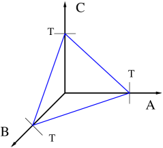
Fig. 1: Positive stoichiometric compatibility class $P$ for chemical reaction system (8).

The three facets (edges) of each positive stoichiometric compatibility class $P$ are one-dimensional line segments:

$$F_{\{A\}} =\left\{~{}(0,x_{b},x_{c})\in\mathbb{R}^{3}_{\geq 0}~{}|~{}x_{b}+x_{c}=T~{}\right\}~{},$$

$$F_{\{B\}} =\left\{~{}(x_{a},0,x_{c})\in\mathbb{R}^{3}_{\geq 0}~{}|~{}x_{a}+x_{c}=T~{}\right\}~{},$$

$$F_{\{C\}} =\left\{~{}(x_{a},x_{b},0)\in\mathbb{R}^{3}_{\geq 0}~{}|~{}x_{a}+x_{b}=T~{}\right\}~{},$$

and the three vertices are the three points $F_{\{A,B\}}=\{(0,0,T)\}$, $F_{\{A,C\}}=\{(0,T,0)\}$, and $F_{\{B,C\}}=\{(T,0,0)\}$. Finally, the set $Z_{\{A,B,C\}}=\{(0,0,0)\}$ is stoichiometrically unattainable. We will revisit this reaction network in Example 5.1.

2.4 Persistence and semilocking sets

Let $x(t)$ be a solution to (4) with strictly positive initial condition $x^{0}\in\mathbb{R}^{N}_{>0}$. The set of $\omega$-limit points for this trajectory is the set of accumulation points:

$$\omega(x^{0})~{}:=~{}\{~{}x\in\mathbb{R}^{N}_{\geq 0}~{}|~{}x(t_{n})\to{x,}\text{ for some sequence }t_{n}\to\infty~{}\}.$$ (10)

Definition 2.11.

A bounded trajectory with initial condition $x^{0}$ is said to be persistent if $\omega(x^{0})\cap\partial\mathbb{R}^{N}_{\geq 0}=\emptyset$. A dynamical system with bounded trajectories is persistent if each trajectory with strictly positive initial condition is persistent.

In order to show that a system is persistent, we must understand which points on the boundary of a positive stoichiometric class are capable of being $\omega$-limit points. To this end, we recall the following definition from the literature.

Definition 2.12.

A nonempty subset $W$ of the set of species is called a semilocking set if for each reaction in which there is an element of $W$ in the product complex, there is an element of $W$ in the reactant complex.

Remark 3.

The notion of a semilocking set is the same as a siphon in the Petri net literature. See [3, 4, 21].

The intuition behind semilocking sets lies in the following proposition, which is the content of Proposition 5.5 of D. Angeli et al. [4]. Related results that concern the “reachability” of species include Theorems 1 and 2 in the textbook of A. Vol´pert and S. Khudi͡aev [24, Section 12.2.3].

Proposition 2.13 ([4]).

Let $W\subset\mathcal{S}$ be non-empty. Then $W$ is a semilocking set if and only if the face $F_{W}$ is forward invariant for the dynamics (4).

The above result holds because semilocking sets are characterized by the following property: if no species of $W$ are present at time zero, then no species of $W$ can be produced at any time in the future. In other words, these species are “locked” at zero for all time. If in addition the reaction network is weakly reversible, then it is straightforward to conclude the following: if a linkage class has a complex whose support contains an element of $W$, then the rates of all reactions within that linkage class will be zero for all positive time: $\kappa_{k}x^{y_{k}}=0$ for any such reaction $y_{k}\to y_{k}^{\prime}$. In other words, certain linkage classes are “shut off.”

In light of the characterization of the interior of a face $F_{W}$ given in (7), the following theorem is proven in [2, 4]; it states that the semilocking sets are the possible sets of zero-coordinates of boundary $\omega$-limit points.

Theorem 2.14 ([2, 4]).

Let $W\subset\mathcal{S}$ be a nonempty subset of the set of species. Let $x^{0}\in\mathbb{R}^{N}_{>0}$ be a strictly positive initial condition for the system (4), and let $P=(x^{0}+S)\cap\mathbb{R}^{N}_{\geq 0}$ denote the corresponding positive stoichiometric compatibility class. If there exists an $\omega(x^{0})$-limit point, $z\in\omega(x^{0})$, and a subset of the species, $W$, such that $z$ is contained within the interior of the face $F_{W}$ of $P$, then $W$ is a semilocking set.

Theorem 2.14 will be used in conjunction with results in the next section to prove the persistence of the following class of weakly reversible systems: those for which each semilocking set $W$ satisfies $\text{dim}(F_{W})=\text{dim}(P)-1$ (and so $F_{W}$ is a facet of $P$) or $F_{W}=\emptyset$ (and so $Z_{W}$ is stoichiometrically unattainable); see Theorem 3.4.

3 Main results

In order to state Theorem 3.2, we need the following definition.

Definition 3.1.

Let $Q\subset P$ be an open set relative to $P$, for which $\emptyset\neq Q\cap\partial P\subset F_{W}$, for some face $F_{W}$ of $P$. Then the face $F_{W}$ is repelling in the neighborhood $Q\cap\operatorname{int}(P)$ with respect to the dynamics (4) if

$$\sum_{i\in W}x_{i}f_{i}(x)~{}\geq~{}0$$ (11)

for all $x\in Q\cap\operatorname{int}(P)$, where the $f_{i}$ are the functions given in (4).

Remark 4.

Note that $F_{W}$ is repelling in the neighborhood $Q\cap\operatorname{int}(P)$ with respect to (4) if and only if $\frac{d}{dt}\operatorname{dist}\left(x(t),F_{W}\right)\geq 0$ whenever $x(t)\in Q\cap\operatorname{int}(P)$. Thus, $F_{W}$ is repelling in a neighborhood if any trajectory in the neighborhood can not get closer to the face $F_{W}$ while remaining in the neighborhood.

The following theorem is our main technical result.

Theorem 3.2.

Let $\{\mathcal{S},\mathcal{C},\mathcal{R}\}$ be a weakly reversible chemical reaction network with dynamics governed by mass action kinetics (4). Let $W\subset\mathcal{S}$ be such that $F_{W}$ is a facet of $P$, and take $z$ to be in the interior of $F_{W}$. Then there exists a $\delta>0$ for which the facet $F_{W}$ is repelling in the neighborhood $B_{\delta}(z)\cap\operatorname{int}(P)$, where $B_{\delta}(z)$ is the open ball of radius $\delta$ centered at the point $z$.

Proof.

For the time being we will assume that there is only one linkage class in the reaction diagram. The proof of the more general case is similar and will be discussed at the end. Also we assume that $W=\{X_{1},\dots,X_{M}\}$ for some $M\leq N$.

Letting $s:=\dim(S)=\dim(P)$, the facet $F_{W}$ has dimension $s-1$, which, by definition, means that $Z_{W}\cap S$ is an $(s-1)$-dimensional subspace of $S$. Let $\pi~{}:~{}\mathbb{R}^{N}\rightarrow\mathbb{R}^{N}$ be the projection onto the first $M$ coordinates, that is, it is given by $\pi(x_{1},x_{2},\dots,x_{M},x_{M+1},\dots,x_{N}):=(x_{1},x_{2},\dots,x_{M},0,\dots,0)$. As a shorthand we will also write $x|_{W}$ for $\pi(x)$. Because $Z_{W}\cap S=\ker(\pi|_{S})$ has dimension $(s-1)$, it follows that the image $\pi(S)$ is one-dimensional. Therefore, we may let $v\in S$ be such that $v|_{W}$ spans the projection $\pi(S)$. We also let $\{w_{2},\dots,w_{s}\}$ span the subspace $Z_{W}\cap S$ so that $\{v,w_{2},\dots,w_{s}\}$ is a basis for the subspace $S$. We simply note for future reference that by construction we have

$$y^{\prime}|_{W}-y|_{W}~{}\in~{}\text{span}(v|_{W})~{},$$ (12)

for each reaction $y\to y^{\prime}\in\mathcal{R}$. Finally, for $x\in\mathbb{R}^{N}$ we define $x|_{W^{c}}$ similarly to $x|_{W}$; that is, $x|_{W^{c}}$ is the projection of $x$ onto the final $N-M$ coordinates.

We may assume that all coordinates of $v|_{W}$ are non-zero, for otherwise the concentrations of certain species $X_{j}\in W$ would remain unchanged under the action of each reaction (note that we necessarily have $w_{k\,i}=0$ for $k\in\{2,\dots,s\}$ and $i\in\{1,\dots,M\}$). In such a case, the concentrations of those species $X_{j}$ would remain constant in time, so we could simply remove them from the system by incorporating their concentrations into the rate constants appropriately.

We will show that $v|_{W}$ has coordinates all of one sign and will use this fact to guarantee the existence of a “minimal complex” (with respect to the elements of $W$). We will then show that this minimal complex corresponds with a dominating monomial that appears as a positive term in each of the first $M$ components of (4).

Suppose, in order to find a contradiction, that $v|_{W}$ has coordinates of both positive and negative sign; that is, assume that $v_{i}<0<v_{j}$ for some indices $i,\ j\leq M$. Let $u:=v_{j}e_{i}-v_{i}e_{j}\in\mathbb{R}^{N}_{\geq 0}$ (where $e_{l}$ denotes the $l$th canonical basis vector). It follows that $u\in S^{\perp}$ because $(i)$ $\langle u,v\rangle=0$ by construction, and $(ii)$ $\langle u,w_{k}\rangle=0$ for all $k\in\{2,\dots,s\}$ because these vectors have non-overlapping support. Note also that $\langle u,z\rangle=0$ because the support of $u$ is a subset of $W$ whereas the support of $z$ is $W^{c}$. Let $x^{0}\in\mathbb{R}^{N}_{>0}\cap P$ (such a point always exists by Remark 1). As $z$ and $x^{0}$ both lie in $P$, there exist constants $\alpha_{k}\in\mathbb{R}$ for $k\in[s]$, such that

$$z=x^{0}+\alpha_{1}v+\sum_{k=2}^{s}\alpha_{k}w_{k}~{}.$$

Combining all of the above we conclude that

$$0~{}=~{}\langle u,z\rangle~{}=~{}\langle u,x^{0}\rangle+\alpha_{1}\langle u,v\rangle+\sum_{k=2}^{s}\alpha_{k}\langle u,w_{k}\rangle=\langle u,x^{0}\rangle~{}>~{}0~{},$$

where the final inequality holds because $u$ is non-negative and nonzero and $x^{0}$ has strictly positive components. This is a contradiction, so we conclude that $v|_{W}$ does not have both positive and negative coordinates, and, without loss of generality, we now assume that all coordinates of $v|_{W}$ are positive.

We recall from (12) that $y^{\prime}|_{W}-y|_{W}~{}\in~{}\text{span}(v|_{W})$ for each reaction $y\to y^{\prime}\in\mathcal{R}$. For concreteness we let ${y^{\prime}_{k}}|_{W}-{y_{k}}|_{W}=\gamma_{k}v|_{W}$ for some $\gamma_{k}\in\mathbb{R}$ where $k\in[R]$. Combining this with the fact that $v_{i}>0$ for each $i\in\{1,\dots,M\}$ shows that each reaction yields either $(i)$ a net gain of all species of $W$, $(ii)$ a net loss of all species of $W$, or $(iii)$ no change in any species of $W$ and, moreover, that there exists a $\tilde{y}\in\mathcal{C}$ such that $\tilde{y}|_{W}\preceq y|_{W}$ for all $y\in\mathcal{C}$, where we say $x\preceq y$ for $x,y\in\mathbb{R}^{N}$ if $x_{i}\leq y_{i}$ for each $i$. Note that it is the sign of $\gamma_{k}$ that determines whether a given reaction accounts for an increase or decrease in the abundances of the elements of $W$.

We now find a neighborhood of positive radius $\delta$ around $z$, $B_{\delta}(z)$, for which the facet $F_{W}$ is repelling in the neighborhood $B_{\delta}(z)\cap\text{int}(P)$. The first condition we impose on $\delta$ is that it must be less than the distance between $z$ and any proper face of $P$ that is not $F_{W}$, which can be done because $z$ is in the interior of the facet. Also, this condition ensures that for any point $x\in B_{\delta}(z)\cap\text{int}(P)$, the coordinates $x_{i}$, for $i>M$, are uniformly bounded both above and below. Therefore, there exist constants $D_{\text{min}}$ and $D_{\text{max}}$ such that for all $x\in B_{\delta}(z)\cap\text{int}(P)$ and all complexes $y$, we have the inequalities

$$0~{}<~{}D_{\text{min}}~{}<~{}x|_{W^{c}}^{y|_{W^{c}}}~{}<~{}D_{\text{max}}~{}.$$ (13)

The monomial $x|_{W}^{\tilde{y}|_{W}}$ will dominate all other monomials for $x\in B_{\delta}(z)\cap\text{int}(P)$ for sufficiently small $\delta$, and this will force trajectories away from the facet. To make this idea precise, let $R_{+}$ denote those reactions that result in a net gain of the species in $W$ and $R_{-}$ those that result in a net loss. We will write $y_{k}\to y_{k}^{\prime}\in R_{+}$ and $y_{k}\to y_{k}^{\prime}\in R_{-}$ to enumerate over those reactions. We now have that for $i\in[M]$ and $x\in B_{\delta}(z)\cap\text{int}(P)$ and for sufficiently small $\delta>0$,

$$\begin{split}f_{i}(x)~{}&=~{}v_{i}\sum_{y_{k}\to y_{k}^{\prime}\in R_{+}}\gamma_{k}\kappa_{k}x|_{W}^{{y_{k}}|_{W}}x|_{W^{c}}^{{y_{k}}|_{W^{c}}}~{}-~{}v_{i}\sum_{y_{k}\to y_{k}^{\prime}\in R_{-}}\left|\gamma_{k}\right|\kappa_{k}x|_{W}^{{y_{k}}|_{W}}x|_{W^{c}}^{{y_{k}}|_{W^{c}}}\\ ~{}&\geq~{}v_{i}D_{\text{min}}\sum_{y_{k}\to y_{k}^{\prime}\in R_{+}}\gamma_{k}\kappa_{k}x|_{W}^{{y_{k}}|_{W}}~{}-~{}v_{i}D_{\text{max}}\sum_{y_{k}\to y_{k}^{\prime}\in R_{-}}\left|\gamma_{k}\right|\kappa_{k}x|_{W}^{{y_{k}}|_{W}}~{}.\end{split}$$ (14)

Finally, by weak reversibility (and possibly after choosing a different $\tilde{y}$ that still satisfies the minimality condition), there is a reaction $\tilde{y}\to y^{\prime}\in\mathcal{R}$ with $\tilde{y}_{i}<y^{\prime}_{i}$ for all $i\in\{1,\dots,M\}$ (i.e. the $\gamma_{k}$ associated with this reaction is strictly positive). This reaction, which belongs to $R_{+}$, has a monomial, $x|_{W}^{\tilde{y}|_{W}}$, that necessarily dominates all monomials associated with reactions in $R_{-}$ (which necessarily have source complexes that contain a higher number of each element of $W$ than $\tilde{y}$ does). Combining this fact with (14) shows that $f_{i}(x)\geq 0$ for $i\in[M]$ and for $x\in B_{\delta}(z)\cap\text{int}(P)$, and therefore, the facet $F_{W}$ is repelling in the neighborhood $B_{\delta}(z)\cap\text{int}(P)$.

In the case of more than one linkage class, each linkage class will have its own minimal complex that will dominate all other monomials associated with that linkage class. Thus the desired result follows. ∎

Remark 5.

Note that weak reversibility was used in the previous proof only to guarantee the existence of the reaction $\tilde{y}\to y^{\prime}$, where $\tilde{y}|_{W}$ is minimal and $\tilde{y}_{i}<y^{\prime}_{i}$ for all $i\in\{1,\dots,M\}$, and was not needed to prove the existence of such a $\tilde{y}$. If the network were not weakly reversible, but such a reaction nevertheless existed, then the same proof goes through unchanged.

Corollary 3.3.

Let $\{\mathcal{S},\mathcal{C},\mathcal{R}\}$ be a weakly reversible chemical reaction network with dynamics governed by mass action kinetics (4) such that all trajectories are bounded. Suppose there exists a subset $W\subset\mathcal{S}$, a positive initial condition $x^{0}\in\mathbb{R}^{N}_{>0}$, and a point $z\in\omega(x^{0})\cap F_{W}$ such that $F_{W}$ is a facet of $P$. Then $\omega(x^{0})\cap\partial F_{W}\neq\emptyset$.

Proof.

Suppose not. That is, suppose that $\omega(x^{0})\cap F_{W}\subset\text{int}(F_{W})$ holds. Let $\mathcal{Y}:=\omega(x^{0})\cap F_{W}$. We claim that $\mathcal{Y}$ is a compact set; indeed, the trajectory $x(t)$ is bounded so $\mathcal{Y}$ is as well, and $\mathcal{Y}$ is the intersection of two closed sets, and therefore is itself closed.

Combining the compactness of $\mathcal{Y}\subset\text{int}(F_{W})$ with Theorem 3.2, we obtain that there exists an open covering of $\mathcal{Y}$ consisting of a finite number of balls $B_{\delta_{i}}(z_{i})$ of positive radius $\delta_{i}$, each centered around an element $z_{i}$ of $\mathcal{Y}$, such that $(i)$ each $\delta_{i}$ is sufficiently small so that $\overline{B_{\delta_{i}}(z_{i})}\,\cap\,\partial F_{W}=\emptyset$, and $(ii)$, for $Q:=\cup_{i}B_{\delta_{i}}(z_{i})$, the facet $F_{W}$ is repelling in $Q\cap\text{int}(P)$. Combining these facts with the existence of $z\in\omega(x^{0})\cap\text{int}(F_{W})\cap Q$ shows the existence of a point $w\in\omega(x^{0})\cap\text{int}(F_{W})\cap\partial Q$. However, this is impossible because $w\in\omega(x^{0})\cap\text{int}(F_{W})=\mathcal{Y}$ necessitates that $w\in\mathcal{Y}\subset\text{int}(Q)$. Thus, the claim is shown. ∎

We may now present our main qualitative result.

Theorem 3.4.

Let $\{\mathcal{S},\mathcal{C},\mathcal{R}\}$ be a weakly reversible chemical reaction network with dynamics governed by mass action kinetics (4) such that all trajectories are bounded. Suppose that for each semilocking set $W$, the corresponding face $F_{W}$ is either a facet ($\text{dim}(F_{W})=\text{dim}(P)-1$) or is empty. Then the system is persistent.

Proof.

This is an immediate consequence of Theorem 2.14 and Corollary 3.3. ∎

3.1 Connection to dynamically non-emptiable semilocking sets

In [3] the notion of a “dynamically non-emptiable” semilocking set is introduced. If for a given semilocking set $W$ we define two sets

$$C(W) :=\left\{~{}0\preceq\alpha\in\mathbb{R}^{R}_{\geq 0}\,:\,w=\sum_{k=1}^{R}\alpha_{k}(y^{\prime}_{k}-y_{k})\text{ satisfies }w|_{W}\preceq 0~{}\right\}\text{~{}and}$$

$$\mathcal{F}_{\epsilon}(W) :=\left\{~{}0\preceq\alpha\in\mathbb{R}^{R}_{\geq 0}\,:\,\alpha_{j}\leq\epsilon\alpha_{i},~{}\forall i,j\in[R]\text{ such that }{y_{i}}|_{W}\precneqq{y_{j}}|_{W}~{}\right\}~{},$$

then $W$ is said to be dynamically non-emptiable if $C(W)\,\cap\,\mathcal{F}_{\epsilon}(W)=\{0\}$ for some $\epsilon>0$. Here the notation $z\preceq z^{\prime}$ means that all coordinates satisfy the inequality $z_{i}\leq z_{i}^{\prime}$ and $z\precneqq z^{\prime}$ means that furthermore at least one inequality is strict. Intuitively, this condition guarantees that all the concentrations of species of a semilocking set can not simultaneously decrease while preserving the necessary monomial dominance. D. Angeli et al. proved that if every semilocking set is dynamically non-emptiable, and if another condition holds (see [3] for details), then the system is persistent.

We next prove that equation (14) and a slight variant of the surrounding argument can be used to show that any semilocking set $W$ associated with a facet of a weakly reversible system is dynamically non-emptiable. We therefore have provided a large set of examples of dynamically non-emptiable semilocking sets.

Corollary 3.5.

Let $\{\mathcal{S},\mathcal{C},\mathcal{R}\}$ be a weakly reversible chemical reaction network with dynamics governed by mass action kinetics (4). Then any semilocking set associated with a facet is dynamically non-emptiable.

Proof.

As in the proof of Theorem 3.2, we may assume that there is one linkage class. The case of more than one linkage class is similar. Let $W=\{X_{1},\dots,X_{M}\}$ be a semilocking set such that $F_{W}$ is a facet. Let $0\neq\alpha\in\mathcal{F}_{\epsilon}(W)$ for some $\epsilon>0$ which may be made smaller as needed. Let $v\in\mathbb{R}^{N}_{\geq 0}$, with $v_{i}>0$ if $i\in[M]$, be as in the proof of Theorem 3.2; that is, $y^{\prime}|_{W}-y|_{W}~{}\in~{}\text{span}(v|_{W})$ for each reaction $y\to y^{\prime}\in\mathcal{R}$ and ${y^{\prime}_{k}}|_{W}-{y_{k}}|_{W}=\gamma_{k}v|_{W}$ for some $\gamma_{k}\in\mathbb{R}$ where $k\in[R]$. Then, for $w$ as in the definition of $C(W)$, and $R_{+}$ and $R_{-}$ defined similarly as in the proof of Theorem 3.2, we have

$$w|_{W}~{}=~{}\sum_{k}\alpha_{k}(y_{k}^{\prime}|_{W}-y_{k}|_{W})~{}=~{}v|_{W}\sum_{y_{k}\to y_{k}^{\prime}\in R_{+}}\alpha_{k}\gamma_{k}~{}-~{}v|_{W}\sum_{y_{k}\to y_{k}^{\prime}\in R_{-}}\alpha_{k}|\gamma_{k}|~{},$$

and so for $i\in\{1,\dots,M\},$

$$w_{i}~{}=~{}v_{i}\sum_{y_{k}\to y_{k}^{\prime}\in R_{+}}\alpha_{k}\gamma_{k}~{}-~{}v_{i}\sum_{y_{k}\to y_{k}^{\prime}\in R_{-}}\alpha_{k}|\gamma_{k}|~{}.$$ (15)

Just as in the proof of Theorem 3.2, there exists a reaction, the $\ell$th say, $\tilde{y}_{\ell}\to y_{\ell}^{\prime}\in R_{+}$ such that $\tilde{y}_{\ell}\preceq y$ for all $y\in\mathcal{C}$, and $\tilde{y}_{\ell}\neq y_{k}$ if $y_{k}\to y_{k}^{\prime}\in R_{-}$. Thus, for $\epsilon>0$ small enough, and by the definition of $\mathcal{F}_{\epsilon}(W)$, the absolute value of the entire negative term in (15) is less than or equal to $v_{\text{min}}\alpha_{\ell}\gamma_{\ell}$, where $v_{\text{min}}:=\min\{v_{i}\,:\,i\in[M]\}$. Therefore we see that $w|_{W}\succeq 0$. If $\alpha_{\ell}=0$, then the preceding argument shows that $\alpha_{k}=0$ for $y_{k}\to y^{\prime}_{k}\in R_{-}$ and so $w_{i}>0$ for all $i\in[M]$ since $\alpha\neq 0$; hence $\alpha\notin C(W)$. For the case $\alpha_{\ell}\neq 0$, it is clear that $w_{i}>0$ for all $i\in[M]$. Thus, we again obtain that $\alpha\notin C(W)$ and the result is shown. ∎

4 The Global Attractor Conjecture

In this section, we use the results of the previous section to resolve some special cases of the Global Attractor Conjecture of chemical reaction network theory. In particular, the main result of this section, Theorem 4.6, establishes that the conjecture holds if all boundary equilibria are confined to the facets and vertices of the positive stoichiometric compatibility classes. That is, the conjecture holds if the faces associated with semilocking sets are facets, vertices, or are empty.

4.1 Complex-balancing systems

The Global Attractor Conjecture is concerned with the asymptotic stability of so-called “complex-balancing” equilibria. Recall that a concentration vector $\overline{x}\in\mathbb{R}^{N}_{\geq 0}$ is an equilibrium of (4) if the differential equations vanish at $\overline{x}$: $f(\overline{x})=0$. For each complex $\eta\in\mathcal{C}$ we will write $\{k\ |\ y_{k}=\eta\}$ and $\{k\ |\ y_{k}^{\prime}=\eta\}$ for the subsets of reactions $k\in\mathcal{R}$ for which $\eta$ is the source and product complex, respectively. In the following definition, it is understood that when summing over the reactions $\{k\ |\ y_{k}^{\prime}=\eta\}$, $y_{k}$ is used to represent the source complex of the given reaction.

Definition 4.1.

An equilibrium $\overline{x}\in\mathbb{R}^{N}_{\geq 0}$ of (4) is said to be complex-balancing if the following equality holds for each complex $\eta\in\mathcal{C}$:

$$\sum_{\{k\ |\ y_{k}=\eta\}}\kappa_{k}({\overline{x}})^{y_{k}^{\prime}}~{}=~{}\sum_{\{k\ |\ y_{k}^{\prime}=\eta\}}\kappa_{k}({\overline{x}})^{y_{k}}~{}.$$

That is, $\overline{x}$ is a complex-balancing equilibrium if, at concentration $\overline{x}$, the sum of reaction rates for reactions for which $\eta$ is the source is equal to the sum of reaction rates for reactions for which $\eta$ is the product. A complex-balancing system is a mass action system (4) that admits a strictly positive complex-balancing equilibrium.

In [6], complex-balancing systems are called “toric dynamical systems” in order to highlight their inherent algebraic structure. Complex-balancing systems are automatically weakly reversible [8]. There are two important special cases of complex-balancing systems: the detailed-balancing systems and the zero deficiency systems.

Definition 4.2.

An equilibrium $\overline{x}\in\mathbb{R}^{N}_{\geq 0}$ of a reversible system with dynamics given by mass action (4) is said to be detailed-balancing if for any pair of reversible reactions $y_{k}\rightleftarrows y_{k}^{\prime}$ with forward reaction rate $\kappa_{k}$ and backward rate $\kappa_{k}^{\prime}$, the following equality holds:

$$\kappa_{k}({\overline{x}})^{y_{k}}=\kappa_{k}^{\prime}({\overline{x}})^{y_{k}^{\prime}}~{}.$$

That is, $\overline{x}$ is a detailed-balancing equilibrium if the forward rate of each reaction equals the reverse rate at concentration $\overline{x}$. A detailed-balancing system is a reversible system with dynamics given by mass action (4) that admits a strictly positive detailed-balancing equilibrium.

Properties of detailed-balancing systems are described by Feinberg in [10] and by A. Vol´pert and S. Khudi͡aev in [24, Section 12.3.3]. It is clear that detailed-balancing implies complex-balancing.

Definition 4.3.

For a chemical reaction network $\{\mathcal{S},\mathcal{C},\mathcal{R}\}$, let $n$ denote the number of complexes, $l$ the number of linkage classes, and $s$ the dimension of the stoichiometric subspace, $S$. The deficiency of the reaction network is the integer $n-l-s$.

The deficiency of a reaction network is non-negative because it can be interpreted as either the dimension of a certain linear subspace [9] or the codimension of a certain ideal [6]. Note that the deficiency depends only on the reaction network or the reaction diagram. It is known that any weakly reversible dynamical system (4) whose deficiency is zero is complex-balancing, and that this fact is independent of the choice of rate constants $\kappa_{k}$ [9]. On the other hand, a reaction diagram with a deficiency that is positive may give rise to a system that is both complex- and detailed-balancing, complex- but not detailed-balancing, or neither, depending on the values of the rate constants $\kappa_{k}$ [6, 8, 10, 15].

4.2 Qualitative behavior of complex-balancing systems

Much is known about the limiting behavior of complex-balancing systems. In the interior of each positive stoichiometric compatibility class $P$ for such a system, there exists a unique equilibrium $\overline{x}$, with strictly positive components, and this equilibrium is complex-balancing. As previously stated, $\overline{x}$ is called the Birch point due to the connection to Birch’s Theorem (see Theorem 1.10 of [20]). Note that a system was defined to be complex-balancing if at least one such equilibrium exists; we now are asserting that so long as at least one $P$ contains a complex-balancing equilibrium, then they all do. As for the stability of the equilibrium within the interior of the corresponding $P$, a strict Lyapunov function exists for each such point. Hence local asymptotic stability relative to $P$ is guaranteed; see Theorem 6A of [16] and the Deficiency Zero Theorem of [9]. The Global Attractor Conjecture states that this equilibrium of $P$ is globally asymptotically stable relative to the interior of $P$ [6]. In the following statement, a global attractor for a set $V$ is a point $v^{*}\in V$ such that any trajectory $v(t)$ with initial condition $v^{0}\in V$ converges to $v^{*}$, in other words, $\lim\limits_{t\rightarrow\infty}v(t)=v^{*}$.

Global Attractor Conjecture For any complex-balancing system (4) and any strictly positive initial condition $x^{0}$, the Birch point $\overline{x}\in P:=(x^{0}+S)\cap\mathbb{R}_{\geq 0}^{N}$ is a global attractor of the interior of the positive stoichiometric compatibility class, $\operatorname{int}(P)$.

This conjecture first appeared in a paper of F. Horn [14], and was given the name “Global Attractor Conjecture” by G. Craciun et al. [6]. It is stated to be the main open question in the area of chemical reaction network theory by L. Adleman et al. [1]. In fact, M. Feinberg stated the more general conjecture that all weakly reversible systems are persistent [9, Section 6.1]. To this end, G. Gnacadja proved that the class of networks of “reversible binding reactions” are persistent; these systems include non-complex-balancing ones [11].

We now describe known partial results regarding the Global Attractor Conjecture. By an interior trajectory we shall mean a solution $x(t)$ to (4) that begins at a strictly positive initial condition $x^{0}\in\mathbb{R}^{N}_{>0}$. It is known that trajectories of complex-balancing systems converge to the set of equilibria; see Corollary 2.6.4 of [5] or Theorem 1 of [23]. Hence, the conjecture is equivalent to the following statement: for a complex-balancing system, any boundary equilibrium is not an $\omega$-limit point of an interior trajectory. It clearly follows that if a positive stoichiometric compatibility class $P$ has no boundary equilibria, then the Global Attractor Conjecture holds for this $P$. Thus, sufficient conditions for the non-existence of boundary equilibria are conditions for which the Global Attractor Conjecture holds (see Theorem 2.9 of [2]); a result of this type is Theorem 6.1 of L. Adleman et al. [1]. Recall that by Theorem 2.14, we know that the only faces $F_{W}$ of a positive stoichiometric compatibility class $P$ that may contain $\omega$-limit points in their interiors are those for which $W$ is a semilocking set. In particular, if the set $Z_{W}$ is stoichiometrically unattainable for all semilocking sets $W$, then $P$ has no boundary equilibria, and hence, the Global Attractor Conjecture holds for this $P$; see the main theorem of D. Angeli et al. [4]. Biological models in which the non-existence of boundary equilibria implies global convergence include the ligand-receptor-antagonist-trap model of G. Gnacadja et al. [12], the enzymatic mechanism of D. Siegel and D. MacLean [22], and the T-cell signal transduction model of T. McKeithan [19] (the mathematical analysis appears in the work of E. Sontag [23] and in the Ph.D. thesis of M. Chavez [5, Section 7.1]). We remark that this type of argument first appeared in [7, Section 6.1].

The remaining case of the Global Attractor Conjecture, in which equilibria exist on the boundary of $P$, is still open. However, some progress has been made. For example, it already is known that vertices of $P$ can not be $\omega$-limit points even if they are equilibria; see Theorem 3.7 in the work of D. Anderson [2] or Proposition 20 of the work of G. Craciun et al. [6]. For another class of systems for which the Global Attractor Conjecture holds despite the presence of boundary equilibria, see Proposition 7.2.1 of the work of M. Chavez [5]. The hypotheses of this result are that the set of boundary equilibria in $P$ is discrete, that each boundary equilibrium is hyperbolic with respect to $P$, and that a third, more technical condition holds. In addition, the Global Attractor Conjecture holds in the case that the network is detailed-balancing, $P$ is two-dimensional, and the network is conservative (meaning that $P$ is bounded); see Theorem 23 of [6]. In the next section, Corollary 4.7 will allow us to eliminate the hypotheses “detailed-balancing” and “conservative” from the two-dimensional result; such partial results concerning the Global Attractor Conjecture are the next topic of this paper.

4.3 Applications to complex-balancing systems

Theorem 4.6 is our main contribution to the Global Attractor Conjecture and generalizes the known results described in Section 4.2. We first present a definition and a lemma.

Definition 4.4.

Suppose that $\{\mathcal{S},\mathcal{C},\mathcal{R}\}$ is a weakly reversible chemical reaction network, endowed with mass action kinetics, and $W\subset\mathcal{S}$ is a semilocking set. Then, the $W$-reduced network is the chemical reaction network $\{\mathcal{S}\setminus W,\tilde{\mathcal{C}},\tilde{\mathcal{R}}\}$ such that $\tilde{\mathcal{C}}$ and $\tilde{\mathcal{R}}$ are those complexes and reactions that do not involve a species from $W$. Equivalently, this is the subnetwork obtained by removing all linkage classes that contain a complex with a species from $W$ in its support. The $W$-reduced system is the $W$-reduced network endowed with the same rate constants as in the original system.

As noted in comments following Proposition 2.13, for a weakly reversible system and any semilocking set $W$, either each complex in a given linkage class contains an element of $W$ or each complex in that linkage class does not contain any element of $W$. Therefore, $W$-reduced systems are themselves weakly reversible. Furthermore, it is easy to check that any $W$-reduced system of a complex-balancing system is itself complex-balancing.

Lemma 4.5.

Consider a complex-balancing system. A face $F_{W}$ of a stoichiometric compatibility class $P$ contains an equilibrium in its interior if and only if $W$ is a semilocking set.

Proof.

It is clear that if a face $F_{W}$ contains an equilibrium in its interior, then $W$ is a semilocking set (see the discussion following Proposition 2.13 or the proof of Theorem 2.5 of [2]).

If $W$ is a semilocking set, then the $W$-reduced system is complex-balancing and one of its invariant polyhedra is naturally identified with $F_{W}$. Therefore, this reduced system admits a complex-balancing equilibrium, which we denote by $y$. For $i\in W^{c}$, let $z_{i}$ be the component of $y$ associated with species $i$. For $i\in W$, let $z_{i}=0$. So constructed, the concentration vector $z$ is an equilibrium within the interior of $F_{W}$. ∎

Theorem 4.6.

The Global Attractor Conjecture holds for any complex-balancing (and in particular, detailed-balancing or weakly reversible zero deficiency) chemical reaction system whose boundary equilibria are confined to facet-interior points or vertices of the positive stoichiometric compatibility classes. Equivalently, if a face $F_{W}$ is a facet, vertex, or an empty face whenever $W$ is a semilocking set, then the Global Attractor Conjecture holds.

Proof.

The equivalence of the two statements in the theorem is a consequence of Lemma 4.5. As noted in the previous section, persistence is a necessary and sufficient condition for the Global Attractor Conjecture to hold. Further, by the results in [2] or [6], vertices may not be $\omega$-limit points. The remainder of the proof is similar to that of Theorem 3.4 and is omitted. ∎

We note that Theorem 4.6 and previous results in [2, 6] show that for equilibria $z$ of complex-balancing systems that reside within the interiors of facets or of vertices of $P$, these faces are repelling near $z$. More precisely, there exists a relatively open set $Q$ of $P$ such that $Q$ contains $z$ and the face is repelling in $Q\cap\operatorname{int}(P)$.

The following corollary resolves the Global Attractor Conjecture for systems of dimension two; note that the one-dimensional case is straightforward to prove.

Corollary 4.7 (GAC for two-dimensional $P$).

The Global Attractor Conjecture holds for all complex-balancing (and in particular, detailed-balancing or weakly reversible zero deficiency) chemical reaction systems whose positive stoichiometric compatibility classes are two-dimensional.

Proof.

This follows immediately from Theorem 4.6 as each face of a two-dimensional polytope must be either a facet or a vertex. ∎

In the next section, we provide examples that illustrate our results, as well as a three-dimensional example for which our results do not apply.

5 Examples

As discussed in the previous section, the Global Attractor Conjecture previously has been shown to hold if $P$ has no boundary equilibria or if the boundary equilibria are restricted to vertices of $P$. Therefore, the examples in this section that pertain to complex-balancing systems feature non-vertex boundary equilibria. Also, we have chosen examples for which the conditions of the theorems can be easily checked.

Example 5.1.

We revisit the network given by the following reactions:

$$2A~{}\underset{\kappa_{2}}{\overset{\kappa_{1}}{\rightleftarrows}}~{}A+B\quad,\quad B~{}\underset{\kappa_{4}}{\overset{\kappa_{3}}{\rightleftarrows}}~{}C~{}.$$

As we saw in Example 2.10, the positive stoichiometric compatibility classes are two-dimensional triangles:

$$P~{}=~{}\left\{~{}(x_{a},x_{b},x_{c})\in\mathbb{R}^{3}_{\geq 0}~{}|~{}x_{a}+x_{b}+x_{c}=T~{}\right\}~{},$$ (16)

where $T>0$. It is straightforward to check that $P$ has a unique boundary equilibrium given by

$$z~{}=~{}\left(0,~{}\frac{\kappa_{4}}{\kappa_{3}+\kappa_{4}}T,~{}\frac{\kappa_{3}}{\kappa_{3}+\kappa_{4}}T\right)~{},$$

and that this point lies in the interior of the facet $F_{\{A\}}$. (Note that this boundary equilibrium is the Birch point of the reversible deficiency zero subnetwork $B\leftrightarrows C$.) Therefore, both Theorem 4.6 and Corollary 4.7 allow us to conclude that despite the presence of the boundary equilibrium $z$, the Birch point in the interior of $P$ is globally asymptotically stable.

We remark that the results in [2] do not apply to the previous example, although Theorem 23 of [6] and Theorem 4 of [3] do. However, for the following example, no previously known results apply.

Example 5.2.

Consider the reaction network depicted below

.

The positive stoichiometric compatibility classes are the same triangles (16) as in the previous example. For each $P$, the set of boundary equilibria is the entire face $F_{\{{A}\}}$ (one of the three edges of $P$), which includes the two vertices $F_{\{A,B\}}$ and $F_{\{A,C\}}$. Hence the results of [2, 5] do not apply. Note that this is a weakly reversible zero deficiency network, but it is not detailed-balancing; so the results of [6] do not apply. Finally, the second condition of Theorem 4 of [3] is not satisfied by this example (there are nested “deadlocks” [3]) and so that result also does not apply. However, both Theorem 4.6 and Corollary 4.7 imply that the Global Attractor Conjecture holds for all choices of rate constants and for all $P$ defined by this network, despite the presence of boundary equilibria.

In the next example, the positive stoichiometric compatibility classes are three-dimensional.

Example 5.3.

The following zero deficiency network is obtained from Example 5.1 by adding a reversible reaction:

$$2A~{}\leftrightarrows~{}A+B~{}\quad,\quad\quad B~{}\leftrightarrows~{}C~{}\leftrightarrows~{}D~{}.$$

The positive stoichiometric compatibility classes are three-dimensional simplices (tetrahedra):

$$P~{}=~{}\left\{~{}(x_{a},x_{b},x_{c},x_{d})\in\mathbb{R}^{4}_{\geq 0}~{}|~{}x_{a}+x_{b}+x_{c}+x_{d}=T~{}\right\}~{},$$

for positive total concentration $T>0$. The unique boundary equilibrium in $P$ is the Birch point of the zero deficiency subnetwork $B\leftrightarrows C\leftrightarrows D$, and it lies in the interior of the facet $F_{\{A\}}$. In other words, the point is $z=(0,x_{b},x_{c},x_{d})$ where $(x_{b},x_{c},x_{d})$ is the Birch point for the system defined by the subnetwork

$$B~{}\leftrightarrows~{}C~{}\leftrightarrows~{}D~{}.$$

Thus by Theorem 4.6 the Global Attractor Conjecture holds for all positive stoichiometric compatibility classes $P$ and all choices of rate constants defined by this network.

As in the previous example, the positive stoichiometric compatibility classes of our next example are three-dimensional. However neither previously known results [2, 5, 6] nor our current results can resolve the question of global asymptotic stability.

Example 5.4.

The following zero deficiency network consists of three reversible reactions:

$$A~{}\leftrightarrows~{}B~{}\leftrightarrows~{}A+B~{}\leftrightarrows~{}A+C~{}.$$

As there are no conservation relations, the unique positive stoichiometric compatibility class is the entire non-negative orthant:

$$P~{}=~{}\mathbb{R}^{3}_{\geq 0}~{}.$$

The set of boundary equilibria is the one-dimensional face (ray) $F_{\{A,B\}}$, which includes the origin $F_{\{A,B,C\}}$. Therefore non-vertex, non-facet boundary equilibria exist, so the results in this paper do not apply.

We end with an example in which the results of Section 3 apply but those of Section 4 do not.

Example 5.5.

The following reversible network is obtained from Example 5.1 by adding another reversible reaction:

$$A+C~{}\underset{\kappa_{2}}{\overset{\kappa_{1}}{\leftrightarrows}}~{}2A~{}\underset{\kappa_{4}}{\overset{\kappa_{3}}{\rightleftarrows}}~{}A+B\quad,\quad B~{}\underset{\kappa_{6}}{\overset{\kappa_{5}}{\rightleftarrows}}~{}C~{}.$$

The positive stoichiometric compatibility classes are again the two-dimensional triangles given by (16). One can easily check that the network has a deficiency of one, so there exist rate constants for which the system is not complex-balancing (for example, $\kappa_{1}=\kappa_{3}$, $\kappa_{5}=\kappa_{6}$, and $\kappa_{2}\neq\kappa_{4}$). Thus the results of Section 4 do not apply. It is also easy to verify that $\{A\}$ and $\{A,B,C\}$ are the only semilocking sets and that $F_{\{A\}}$ is a facet and $F_{\{A,B,C\}}$ is empty. Therefore, Theorem 3.4 applies and we conclude that, independent of the choice of rate constants, the system is persistent.

Acknowledgments

The authors thank Gheorghe Craciun for helpful discussions. This work began during a focused research group hosted by the Mathematical Biosciences Institute at The Ohio State University, and the authors benefited from a subsequent visit to the Statistical and Applied Mathematical Sciences Institute in North Carolina. We also acknowledge the helpful comments of anonymous reviewers, which greatly improved the paper.

References

- [1] Leonard Adleman, Manoj Gopalkrishnan, Ming-Deh Huang, Pablo Moisset, Dustin Reishus. On the mathematics of the law of mass-action. Available from arXiv:0810.1108.
- [2] David F. Anderson. Global asymptotic stability for a class of nonlinear chemical equations, SIAM J. Appl. Math, 68:5, 1464–1476, 2008.
- [3] David Angeli, Patrick De Leenheer, and Eduardo Sontag. A Petri net approach to persistence analysis in chemical reaction networks. In I. Queinnec, S. Tarbouriech, G. Garcia, and S-I. Niculescu, editors, Biology and Control Theory: Current Challenges (Lecture Notes in Control and Information Sciences Volume 357), pages 181–216. Springer-Verlag, Berlin, 2007.
- [4] David Angeli, Patrick De Leenheer, Eduardo Sontag. A Petri net approach to the study of persistence in chemical reaction networks. Math. Biosci., 210 (2007), 598–618.
- [5] Madalena Chavez. Observer design for a class of nonlinear systems, with applications to chemical and biological networks. Ph.D. Thesis, Rutgers University, New Brunswick, NJ, 2003.
- [6] Gheorghe Craciun, Alicia Dickenstein, Anne Shiu, Bernd Sturmfels. Toric Dynamical Systems. J. Symb. Comput., 44, 1551–1565.
- [7] Martin Feinberg. Chemical reaction network structure and the stability of complex isothermal reactors I. The deficiency zero and deficiency one theorems, Chem. Eng. Sci., 42:10, 2229–2268, 1987.
- [8] Martin Feinberg. Complex balancing in general kinetic systems, Arch. Rat. Mech. Anal., 49:3, 187–194, 1972.
- [9] Martin Feinberg. Lectures on chemical reaction networks. Notes of lectures given at the Mathematics Research Center of the University of Wisconsin in 1979, http://www.che.eng.ohio-state.edu/FEINBERG/LecturesOnReactionNetworks.
- [10] Martin Feinberg. Necessary and sufficient conditions for detailed balancing in mass action systems of arbitrary complexity, Chem. Eng. Sci., 44:9, 1819–1827, 1989.
- [11] Gilles Gnacadja. Univalent positive polynomial maps and the equilibrium state of chemical networks of reversible binding reactions. Available from http://math.gillesgnacadja.info/files/Reversible_Binding_Reactions.html.
- [12] Gilles Gnacadja, Alex Shoshitaishvili, Michael Gresser, Brian Varnum, David Balaban, Mark Durst, Chris Vezina, Yu Li. Monotonicity of interleukin-1 receptor-ligand binding with respect to antagonist in the presence of decoy receptor, J. Theor. Biol., 244:478–488, 2007.
- [13] Jeremy Gunawardena. Chemical reaction network theory for in-silico biologists. Technical Report, 2003, http://vcp.med.harvard.edu/papers/crnt.pdf.
- [14] Fritz Horn. The dynamics of open reaction systems. Mathematical aspects of chemical and biochemical problems and quantum chemistry, SIAM-AMS Proceedings, Vol. VIII, 125–137, 1974.
- [15] Fritz Horn. Necessary and sufficient conditions for complex balancing in chemical kinetics, Arch. Rat. Mech. Anal., 49:3, 172–186, 1972.
- [16] Fritz Horn and Roy Jackson. General mass action kinetics. Arch. Rat. Mech. Anal., 47:2, 81–116, 1972.
- [17] Thomas Kurtz. Approximation of population processes. CBMS-NSF Regional Conference Series in Applied Mathematics, Vol. 36, SIAM, Philadelphia, PA, 1981.
- [18] Thomas Kurtz. The relationship between stochastic and deterministic models for chemical reactions. J. Chem. Phys., 57:7, 2976–2978, 1972.
- [19] Timothy McKeithan. Kinetic proofreading in T-cell receptor signal transduction. PNAS, 92:11, 5042–5046, 1995.
- [20] Lior Pachter and Bernd Sturmfels. Algebraic Statistics for Computational Biology, Cambridge University Press, Cambridge, 2005.
- [21] Anne Shiu and Bernd Sturmfels. Siphons in chemical reaction networks. Available from arXiv:0904.4529.
- [22] David Siegel and Debbie MacLean. Global stability of complex balanced mechanisms. J. Math. Chem., 27:1–2, 89–110, 2004.
- [23] Eduardo Sontag. Structure and stability of certain chemical networks and applications to the kinetic proofreading model of T-cell receptor signal transduction, IEEE Trans. Automat. Control, 46: 1028–1047, 2001.
- [24] Aĭzik Vol´pert and Sergeĭ Khudi͡aev. Analysis in Classes of Discontinuous Functions and Equations of Mathematical Physics. Springer, Dordrecht, 1985.
- [25] Günter Ziegler. Lectures on Polytopes. Vol. 152 of Graduate Texts in Mathematics. Springer-Verlag, New York, 1995.