RUNHETC-2008-18

TAUP-2890-08

ITEP-TH-45/08

A Pure-Glue Hidden Valley
I. States and Decays

J. E. Juknevich^a, D. Melnikov^b,c and M. J. Strassler^a
aDepartment of Physics and Astronomy,
Rutgers, 136 Frelinghuysen Rd, Piscataway, NJ 08854, USA
^bRaymond and Beverly Sackler School of Physics and Astronomy,
Tel Aviv University, Ramat Aviv 69978, Israel
^cInstitute for Theoretical and Experimental Physics,
B. Cheremushkinskaya 25, 117259 Moscow, Russia

It is possible that the standard model is coupled, through new massive charged or colored particles, to a hidden sector whose low energy dynamics is controlled by a pure Yang-Mills theory, with no light matter. Such a sector would have numerous metastable “hidden glueballs” built from the hidden gluons. These states would decay to particles of the standard model. We consider the phenomenology of this scenario, and find formulas for the lifetimes and branching ratios of the most important of these states. The dominant decays are to two standard model gauge bosons, or by radiative decays with photon emission, leading to jet- and photon-rich signals.

1 Introduction

With the Large Hadron Collider (LHC), particle physics enters a new era of potential discovery, one which may provide insights into the many puzzles of the standard model (SM). Given the immense challenges of hadron collider physics, and the degree to which the future of particle physics rests on the LHC, it is important to ensure that the LHC community is fully prepared for whatever might appear in the data. This requires consideration of a wide variety of models and signatures in advance of the experimental program.

There are a number of reasonable and motivated solutions to the hierarchy problem, the most favored being supersymmetry (SUSY), with others including the little Higgs, warped extra dimensions and technicolor. Most experimental studies of these ideas have focused on “minimal” models. But unlike supersymmetry or the little Higgs, minimality does not by itself solve any particle physics problem. Instead, it is motivated by theorists’ philosophical attachment to beauty and elegance. Given our experience with the standard model, whose third generation and neutral currents were not viewed as well-motivated before they were discovered, it is prudent that we examine non-minimal models as well, to ensure that their signatures would not be missed at the LHC. This is especially important because a small addition to a theory can lead to a large change in its LHC phenomenology.

One likely possibility for new non-minimal physics involves the presence of a hidden sector with TeV-scale couplings to the standard model. A large fraction of these models fall within the “hidden valley scenario” [1, 2, 3, 4, 5, 6]. In the hidden valley scenario, a new hidden sector (the “hidden valley sector”, or “v-sector” for short) is coupled to the SM in some way at or near the TeV scale, and the v-sector’s dynamics generates a mass gap. Such a mass gap, independent of the dynamics leading to that gap, ensures that there are particles that are stable or metastable within the v-sector. These can only decay, if at all, via their very weak interactions with the SM. Processes that access the hidden valley are often quite unusual compared to those in minimal supersymmetric or other well-studied models. Production of v-sector particles commonly leads to final states with a high multiplicity of SM particles. Also, a hidden valley often leads to particles that decay with macroscopic decay distances. The resulting phenomenological signatures can be difficult, or at least subtle, for detection at the Tevatron or LHC; see for example [1, 2, 6].

Hidden valleys have arisen in bottom-up models such as the twin-Higgs and folded-supersymmetry models [7, 8] that attempt to address the hierarchy problem, and in a recent attempt to explain the various anomalies in dark-matter searches [9] which requires a dark sector with a new force and a 1 GeV mass scale. They are also motivated by top-down model building: hidden sectors that are candidate hidden valleys arise in many string theory models, see for example [10]. In recent years string theorists have found many models that apparently have the minimal supersymmetric standard model as the chiral matter of the theory, but which typically have extra vector-like matter and extra gauge groups. The non-minimal particles and forces which arise in these various models may very well be visible at the LHC [1].

In this paper we consider a hidden valley that at low energy is a pure-Yang-Mills theory, a theory that has its own gluons (“v-gluons”) and their bound states (“v-glueballs”). This scenario easily arises in models; for example, in many supersymmetric v-sectors, supersymmetry breaking and associated scalar expectation values may lead to large masses for all matter fields.

The spectrum of stable bound states in a pure Yang-Mills theory is known, to a degree, from lattice simulations [11]. The spectrum of such states for an $SU(3)$ gauge group is shown in figure 1. The spectrum includes many glueballs of mass of order the confinement scale $\Lambda_{v}$ (actually somewhat larger), and various $J^{PC}$ quantum numbers. All of the states shown are stable against decay to the other states, due to kinematics and/or conserved quantum numbers.

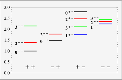
Figure 1: Spectrum of stable glueballs in pure glue $SU(3)$ theory [11].

In this paper we will further specialize to the case where the coupling between the SM sector and the v-sector occurs through a multiplet of massive particles (which we will call $X$) charged under both SM-sector and v-sector gauge groups. A loop of $X$ particles induces dimension-$D$ operators of the form

$$\frac{1}{M^{D-4}}{\cal O}_{s}^{(D-d)}{\cal O}_{v}^{(d)}$$ (1)

where $M$ is the mass of the heavy particle in the loop. Here we have split the dimension-$D$ operator ${\cal O}^{(D)}$ into a Standard-Model part ${\cal O}_{s}^{(D-d)}$ of dimension $D-d$ and a hidden-valley part ${\cal O}_{v}^{(d)}$ of dimension $d$. All v-glueball states can decay through these operators.

By simple dimensional analysis, these operators yield partial decay widths of order $\Lambda_{v}^{2D-7}/M^{2D-8}$. We will see that the v-glueball decays are dominated by $D=8$ operators. The next operators have $D=10$, and their effects are typically suppressed by $\sim(\Lambda_{v}/M)^{4}$. The $D=8$ operators induce lifetimes for the v-glueballs of order $M^{8}/\Lambda^{9}$, which can range anywhere from $10^{-20}$ seconds to much longer than a second, depending on the parameters. Implicitly our focus is on the case where the lifetimes are short enough that at least a few decays can be observed in an LHC detector. This typically requires lifetimes shorter than a micro-second, if the production cross-section is substantial. However, our formulas will be valid outside this regime as well.

We will need to construct the $D=8$ effective action coupling the two sectors. Then we will use it to compute formulas for the partial widths of various decay modes of the v-glueballs, concentrating on the lighter v-glueball states, which we expect to be produced most frequently.

Application of our formulas, particularly as relevant for the LHC, will be carried out in a second paper [15]. To put the present paper in context, we now briefly review the results to be presented there. Although there are some irreducible uncertainties due to unknown glueball transition matrix elements and decay constants, we find that the various v-glueball states have lifetimes that probably span 3 or 4 orders of magnitude. We also find that the dominant v-glueball decays are to SM gauge-boson pairs, or radiative decays to another v-glueball and a photon (or perhaps a $Z$ boson.) We will demonstrate that detection should be straightforward, if the mass $M$ of the quirk $X$ is small enough to give a reasonable cross-section, and $\Lambda_{v}$ is large enough to ensure the v-glueballs decay promptly. Several v-glueballs form di-photon resonances, which should be easy to detect if their decays are prompt. Unlike [5], or especially [6], it appears that traditional cut-based analysis on ordinary events with jets and photons will be sufficient. For displaced decays, however, special experimental techniques are always needed. There are a number of different signatures, and the optimal search strategy is not obvious.

The present paper is organized as follows. In Sec. 2, we introduce our model and systematically describe the v-sector operators and the v-glueball states. In Sec. 3, we describe the effective action coupling the two sectors and the SM matrix elements relevant for the decays. Our main results for the decay modes and their branching fractions appear in Sec. 4. We conclude in Sec. 5 with some final comments and perspective. Additional results appear in the Appendix.

2 The model and the hidden valley sector

2.1 Description of the Model

Consider adding to the standard model (SM) a new gauge group $G$, with a confinement scale $\Lambda_{v}$ in the 1–1000 GeV range. We will refer to this sector as the “hidden valley”, or the “v-sector” following [1]. What makes this particular confining hidden valley special is that it has no light charged matter; its only light fields are its gauge bosons, which we will call “hidden gluons” or “v-gluons”. At low energy, confinement generates (meta)stable bound states, “v-glueballs”, from the v-gluons. The SM is coupled to the hidden valley sector only through heavy fields $X_{r}$, in vector-like representations of both the SM and $G$, with masses of order the TeV scale. These states can be produced directly at the LHC, but because of v-confinement they cannot escape each other; they form a bound state which relaxes toward the ground state and eventually annihilates. The products of the annihilation are often v-glueballs. (Other annihilations lead typically to a hard pair or trio of standard model particles.) Thereafter, the v-glueballs decay, giving a potentially visible signal.

For definiteness, we take the gauge group $G$ to be $SU(n_{v})$, and the particles $X_{r}$ to transform as a fundamental representation of $SU(n_{v})$ and in complete $SU(5)$ representations of the Standard Model, typically ${\bf 5}+{\bf\bar{5}}$ and/or ${\bf 10}+{\bf\overline{10}}$. We label the fields and their masses as shown in table 1.

Field	$SU(3)$	$SU(2)$	$U(1)$	$SU(n_{v})$	Mass
$X_{\bar{d}}$	${\bf 3}$	${\bf 1}$	$\frac{1}{3}$	${\bf n_{v}}$	$m_{\bar{d}}$
$X_{\ell}$	${\bf 1}$	${\bf 2}$	${-\frac{1}{2}}$	${\bf n_{v}}$	$m_{\ell}$
$X_{\bar{u}}$	$\bf\bar{3}$	$\bf 1$	$-\frac{2}{3}$	$\bf n_{v}$	$m_{\bar{u}}$
$X_{q}$	$\bf 3$	$\bf 2$	$\frac{1}{6}$	$\bf n_{v}$	$m_{q}$
$X_{e}$	${\bf 1}$	${\bf 1}$	${\bf 1}$	${\bf n_{v}}$	$m_{e}$

Table 1: The new fermions $X_{r}$ that couple the hidden valley sector to the SM sector.

In this paper, we will calculate their effects as a function of $m_{r}$. The approximate global $SU(5)$ symmetry of the SM gauge couplings suggests that the masses $m_{\bar{d}}$ and $m_{\ell}$ should be roughly of the same order of magnitude, and similarly for the masses $m_{q},m_{\bar{u}},m_{e}$. It is often more convenient to express the answer as a function of the (partially redundant) dimensionless parameters

$$\rho_{r}\equiv m_{r}/M\ .$$ (2)

Here $M$ is a mass scale that can be chosen arbitrarily; depending on parameters, it is usually most natural to take it to be the mass of the lightest $X_{r}$ particle.

Integrating out these heavy particles generates an effective Lagrangian ${\cal L}_{{\rm eff}}$ that couples the v-gluons and the SM gauge bosons. The terms in the effective Lagrangian are of the form (1), with operators ${\cal O}_{v}^{(d)}$ constructed from the gauge invariant combinations ${\rm tr\ }{\cal{F}}_{\mu\nu}{\cal{F}}_{\alpha\beta}$ and ${\rm tr\ }{\cal{F}}_{\mu\nu}{\cal{F}}_{\alpha\beta}{\cal{F}}_{\delta\sigma}$, contracted according to different irreducible representations of the Lorentz group.

The interactions in the effective action then allow the v-glueballs in figure 1, which cannot decay within the v-sector, to decay to final states containing SM particles and at most one v-glueball. This is analogous to the way that the Fermi effective theory, which couples the quark sector to the lepton sector, permits otherwise stable QCD hadrons to decay weakly to the lepton sector. As is also true for leptonic and semileptonic decays of QCD hadrons, our calculations for v-hadrons decaying into SM particles simplify because of the factorization of the matrix elements into a purely SM part and a purely hidden-sector part. To compute the v-glueball decays, we will only need the following factorized matrix elements, involving terms in the effective action of dimension eight:

$$\langle SM|{{\cal O}_{s}^{(8-d)}}|0\rangle\langle 0|{{\cal O}_{v}^{(d)}}|\Theta_{\kappa}\rangle\ ,$$ (3)

$$\langle SM|{{\cal O}_{s}^{(8-d)}}|0\rangle\langle\Theta_{\kappa^{\prime}}|{{\cal O}_{v}^{(d)}}|\Theta_{\kappa}\rangle\ .$$ (4)

Here $d$ is the mass dimension of the operator in the v-sector, $\langle SM|$ schematically represents a state built from Standard Model particles, and $|\Theta_{\kappa}\rangle$ and $|\Theta_{\kappa^{\prime}}\rangle$ refer to v-glueball states with quantum numbers $\kappa$, which include spin $J$, parity $P$ and charge-conjugation $C$. We will see later that we only need to consider $d=4$ and $6$; there are no dimension $D=8$ operators in ${\cal L}_{{\rm eff}}$ for which $d=5$, since there are no appropriate dimension-three SM operators to compensate. The SM part $\langle SM|{{\cal O}_{s}^{(8-d)}}|0\rangle$ can be evaluated by the usual perturbative methods of quantum field theory, but a computation of the hidden-sector matrix elements $\langle 0|{{\cal O}_{v}^{(d)}}|\Theta_{\kappa}\rangle$ and $\langle\Theta_{\kappa^{\prime}}|{{\cal O}_{v}^{(d)}}|\Theta_{\kappa}\rangle$ requires the use of non-perturbative methods.

2.2 Classification of v-glueball states

In this section we shall classify the nonvanishing v-sector matrix elements. A v-glueball state $\Theta_{\kappa}$ with quantum numbers $J^{PC}$ can be created by certain operators ${\cal O}_{v}^{(d)}$ acting on the vacuum $|\,0\rangle$. We wish to know which matrix elements, $\langle 0|{{\cal O}_{v}^{(d)}}|\Theta_{\kappa}\rangle$ and $\langle\Theta_{\kappa}^{\prime}|{{\cal O}_{v}^{(d)}}|\Theta_{\kappa}\rangle$, are nonvanishing. This is equivalent to finding how the operators in various Lorentz representations are projected onto states with given quantum numbers $J^{PC}$. Their classification was carried out in [16]. At mass dimension $d=4$ there are four different operators transforming in irreducible representations of the Lorentz group. These are shown in table 2. From now on, we denote the operators ${\cal O}_{v}^{\xi}$, where $\xi$ runs over different irreducible operators $\xi=S,P,T,L,\cdots$.

Operator ${\cal O}^{\xi}_{v}$	$J^{PC}$
$S={\rm tr\ }{\cal{F}}_{\mu\nu}{\cal{F}}^{\mu\nu}$	$0^{++}$
$P={\rm tr\ }{\cal{F}}_{\mu\nu}\tilde{\cal{F}}^{\mu\nu}$	$0^{-+}$
$T_{\alpha\beta}={\rm tr\ }{\cal{F}}_{\alpha\lambda}{\cal{F}}^{~{}\lambda}_{\beta}-\frac{1}{4}\,g_{\alpha\beta}S$	$2^{++}$, $1^{-+}$, $0^{++}$
$L_{\mu\nu\alpha\beta}={\rm tr\ }{\cal{F}}_{\mu\nu}{\cal{F}}_{\alpha\beta}-\frac{1}{2}\,(g_{\mu\alpha}T_{\nu\beta}+g_{\nu\beta}T_{\mu\alpha}-g_{\mu\beta}T_{\nu\alpha}-g_{\nu\alpha}T_{\mu\beta})$	$2^{++}$, $2^{-+}$
$-\frac{1}{12}\,(g_{\mu\alpha}g_{\nu\beta}-g_{\mu\beta}g_{\nu\alpha})S+\frac{1}{12}\,\epsilon_{\mu\nu\alpha\beta}P$

Table 2: The dimension $d=4$ operators, and the states that can be created by these operators [16]. We denote $\tilde{\cal{F}}_{\mu\nu}=\frac{1}{2}\,\epsilon_{\mu\nu\alpha\beta}{\cal{F}}^{\alpha\beta}$.

The study of irreducible representations of dimension-six operators is more involved. A complete analysis in terms of electric and magnetic gluon fields, $\vec{E}_{a}$ and $\vec{B}_{a}$, was also presented in [16], with a detailed description of the operators and the states contained in their spectrum. There are only two such operators of relevance for our work, which we denote $\Omega^{(1)}_{\mu\nu}$ and $\Omega^{(2)}_{\mu\nu}$ as shown in table 3. The other dimension-six operators simply cannot be combined with any SM operator to make a dimension-eight interaction.

Operator ${\cal O}^{\xi}_{v}$	$J^{PC}$
$\Omega^{(1)}_{\mu\nu}={\rm tr\ }{\cal{F}}_{\mu\nu}{\cal{F}}_{\alpha\beta}{\cal{F}}^{\alpha\beta}$	$1^{--}$, $1^{+-}$
$\Omega^{(2)}_{\mu\nu}={\rm tr\ }{\cal{F}}_{\mu}^{\alpha}{\cal{F}}^{\beta}_{\alpha}{\cal{F}}_{\beta\nu}$	$1^{--}$, $1^{+-}$

Table 3: The important $d=6$ operators. The states that can be created by these operators are shown [16].

2.3 Matrix elements

As we saw, the matrix elements are factorized into a purely SM part and a purely v-sector part. We will first consider the v-sector matrix elements relevant to v-glueball transitions, $\langle 0|{{\cal O}_{v}^{\xi}}|\Theta_{\kappa}\rangle$ and $\langle\Theta_{\kappa^{\prime}}|{{\cal O}_{v}^{\xi}}|\Theta_{\kappa}\rangle$, where $|\Theta_{\kappa}\rangle$ and $|\Theta_{\kappa^{\prime}}\rangle$ refer to v-glueball states with given quantum numbers and ${\cal O}^{\xi}_{v}$ is any of the operators in tables 2 and 3.

It is convenient to write the most general possible matrix element in terms of a few Lorentz invariant amplitudes or form factors. For the annihilation matrix elements we will write

$$\langle 0|{{\cal O}_{v}^{\xi}}|\Theta_{\kappa}\rangle=\Pi_{\kappa,\mu\nu\cdots}^{\xi}{\bf F}_{\kappa}^{\xi}\ ,$$ (5)

where ${\bf F_{\kappa}^{\xi}}$ is the decay constant of the v-glueball $\Theta_{\kappa}$, and $\Pi_{\kappa,\mu\nu\cdots}^{\xi}$ is determined by the Lorentz representations of $\Theta_{\kappa}$ and ${\cal O}_{v}^{\xi}$. In table 4 we list $\Pi_{\kappa,\mu\nu\cdots}^{\xi}$ for each operator.

The decay constants ${\bf F}_{\kappa}^{\xi}$ depend on the internal structure of the v-glueball states and, with the exception of those that vanish due to conservation laws (see footnote 6), must be determined by non-perturbative methods, for instance, by numerical calculations in lattice gauge theory. Only the first three non-vanishing decay constants in table 4 have been calculated, for $SU(3)$ Yang-Mills theory [17], although the reported values are not expressed in a continuum renormalization scheme. The other decay constants have not been computed.

Likewise, the transition matrix elements $\langle\Theta_{\kappa^{\prime}}|{{\cal O}_{v}^{\xi}}|\Theta_{\kappa}\rangle$ are of the form

$$\langle\Theta_{\kappa^{\prime}}|{{\cal O}_{v}^{\xi}}|\Theta_{\kappa}\rangle=\Pi_{\kappa\kappa^{\prime},\mu\nu\cdots}^{\xi}{\bf M}_{\kappa,\kappa^{\prime}}^{\xi},$$ (6)

where now ${\bf M}_{\kappa,\kappa^{\prime}}^{\xi}$ is the transition matrix, which depends only on the transferred momentum. In table 5 we have listed $\Pi_{\kappa\kappa^{\prime},\mu\nu\cdots}^{\xi}$ for the simplest cases considered later in this work. In several other cases more than one Lorentz structure $\Pi_{\kappa\kappa^{\prime},\mu\nu\cdots}^{\xi}$ contributes to the transition element. In such cases, since none of these matrix elements are known from numerical simulation, we will usually simplify the problem by using the lowest partial-wave approximation for the amplitudes. More details will follow in Sec. 4.

${\cal O}^{\xi}_{v}$ ($\Theta_{\kappa}$)	$\Pi_{\kappa,\mu\nu\cdots}^{\xi}$	${\bf F}_{\kappa}^{\xi}$
$S$ $(0^{++})$	$\mathbf{1}$	$\mathbf{F^{S}_{0^{++}}}$
$P$ $(0^{-+})$	$\mathbf{1}$	$\mathbf{F^{P}_{0^{-+}}}$
$T_{\alpha\beta}$ $(0^{++})$	$g_{\alpha\beta}-\frac{p_{\alpha}p_{\beta}}{p^{2}}$	0
$T_{\alpha\beta}$ $(1^{-+})$	$p_{\alpha}\epsilon_{\beta}+p_{\beta}\epsilon_{\alpha}$	0
$T_{\alpha\beta}$ $(2^{++})$	$\epsilon_{\alpha\beta}$	$\mathbf{F^{T}_{2^{++}}}$
$L_{\mu\nu\alpha\beta}$ $(2^{++})$	$\epsilon_{\mu\alpha}\mathcal{P}_{\nu\beta}+\epsilon_{\nu\beta}\mathcal{P}_{\mu\alpha}-\epsilon_{\nu\alpha}\mathcal{P}_{\mu\beta}-\epsilon_{\mu\beta}\mathcal{P}_{\nu\alpha}$	$\mathbf{F^{L}_{2^{++}}}$
$L_{\mu\nu\alpha\beta}$ $(2^{-+})$	$(\epsilon_{\mu\nu\rho\sigma}\epsilon^{\sigma}_{~{}\beta}p^{\rho}p_{\alpha}-\epsilon_{\mu\nu\rho\sigma}\epsilon^{\sigma}_{~{}\alpha}p^{\rho}p_{\beta}$	$\mathbf{F^{L}_{2^{-+}}}$
	$+\epsilon_{\alpha\beta\rho\sigma}\epsilon^{\sigma}_{~{}\nu}p^{\rho}p_{\mu}-\epsilon_{\alpha\beta\rho\sigma}\epsilon^{\sigma}_{~{}\mu}p^{\rho}p_{\nu})/p^{2}$
$\Omega^{(n)}_{\mu\nu}$ $(1^{--})$	$m_{1^{-}}(p_{\mu}\epsilon_{\nu}-p_{\nu}\epsilon_{\mu})$	$\mathbf{F^{\Omega^{(n)}}_{1^{--}}}$
$\Omega^{(n)}_{\mu\nu}$ $(1^{+-})$	$m_{1^{+}}\epsilon_{\mu\nu\alpha\beta}(p^{\alpha}\epsilon^{\beta}-p^{\beta}\epsilon^{\alpha})$	$\mathbf{F^{\Omega^{(n)}}_{1^{+-}}}$

Table 4: Annihilation matrix elements. $\epsilon_{\mu}$ and $\epsilon_{\mu\nu}$ are the polarization vectors of $1^{--},1^{+-}$ and polarization tensor of $2^{++},2^{-+}$ respectively. ${\mathcal{P}}_{\alpha\beta}=g_{\alpha\beta}-2p_{\alpha}p_{\beta}/p^{2}$. $m_{1^{-}},m_{1^{+}}$ are the masses of the $1^{--},1^{+-}$ states; their appearance merely reflects our normalization convention.

${\cal O}^{\xi}_{v}$ ($\Theta_{\kappa}$ $\Theta_{\kappa^{\prime}}$)	$\Pi_{\kappa\kappa^{\prime},\mu\nu\cdots}^{\xi}$	${\bf M}_{\kappa\kappa^{\prime}}^{\xi}$
$P$ $(0^{-+},0^{++})$	$\mathbf{1}$	$\mathbf{M_{0^{+}0^{-}}^{P}}$
$\Omega_{\mu\nu}^{(n)}$ $(1^{--},0^{++})$	$p_{\mu}\epsilon_{\nu}-p_{\nu}\epsilon_{\mu}$	$\mathbf{M_{1^{--}0^{++}}^{\Omega^{(n)}}}$
$\Omega_{\mu\nu}^{(n)}$ $(1^{+-},0^{-+})$	$p_{\mu}\epsilon_{\nu}-p_{\nu}\epsilon_{\mu}$	$\mathbf{M_{1^{+-}0^{-+}}^{\Omega^{(n)}}}$
$\Omega_{\mu\nu}^{(n)}$ $(1^{--},0^{-+})$	$\epsilon_{\mu\nu\alpha\beta}p^{\alpha}\epsilon^{\beta}$	$\mathbf{M_{1^{--}0^{-+}}^{\Omega^{(n)}}}$
$\Omega_{\mu\nu}^{(n)}$ $(1^{+-},0^{++})$	$\epsilon_{\mu\nu\alpha\beta}p^{\alpha}\epsilon^{\beta}$	$\mathbf{M_{1^{+-}0^{++}}^{\Omega^{(n)}}}$
$P$ $(1^{--},1^{+-})$	$\epsilon^{+}\cdot\epsilon^{-}$	$\mathbf{M_{1^{--}1^{+-}}^{P}}$
$L$ $(1^{--},1^{+-})$	$\epsilon_{\mu\nu\rho\sigma}p^{\rho}{\epsilon^{-}}^{\sigma}(p_{\alpha}{\epsilon^{+}}_{\beta}-p_{\beta}{\epsilon^{+}}_{\alpha})+\mu\nu\leftrightarrow\alpha\beta-{\rm traces}$	$\mathbf{M_{1^{--}1^{+-}}^{L}}$
$\Omega_{\mu\nu}^{(n)}$ $(2^{-+},1^{+-})$	$p_{\mu}\epsilon_{\nu\alpha}\epsilon^{\alpha}-p_{\nu}\epsilon_{\mu\alpha}\epsilon^{\alpha}$	$\mathbf{\bf M_{2^{-+}1^{+-}}^{\Omega^{(n)}}}$
$\Omega_{\mu\nu}^{(n)}$ $(1^{+-},2^{++})$	$\epsilon_{\mu\nu\alpha\beta}\epsilon^{\alpha\lambda}\tilde{\epsilon}_{\lambda}p^{\beta}$, $\epsilon_{\mu\nu\alpha\beta}\epsilon^{\alpha\lambda}p_{\lambda}\tilde{\epsilon}^{\beta}$	$\mathbf{\bf M_{1^{+-}2^{++}}^{\Omega^{(n)}}}$

Table 5: Transition matrix elements. Momentum of the final glueball $\Theta_{\kappa^{\prime}}$ is denoted $p^{\mu}$; $\epsilon^{\alpha}$ and $\epsilon^{\alpha\beta}$ are polarization tensors of spin 1 and spin 2 states respectively. The bottom part of the table contains matrix elements in the lowest partial wave approximation.

Clearly, any numerical results arising from our formulas, as we ourselves will obtain in our LHC study [15], will be subject to some large uncertainties, due to the unknown matrix elements. Of course, with sufficient motivation, such as a hint of a discovery, many of these could be determined through additional lattice gauge theory computations.

Now we turn to the SM part of the matrix element, which can be treated perturbatively, since we will only consider v-glueballs with masses well above $\Lambda_{QCD}$. In all of our calculations, the SM gauge-boson field-strength tensors, which appear in the operators, are replaced in the matrix element by the substitution $G_{\mu\nu}\leftrightarrow k_{\mu}\varepsilon_{\nu}-k_{\nu}\varepsilon_{\mu}$. For example, for a transition to two gauge bosons, we write

$$\langle k_{1},\varepsilon^{a}_{1};k_{2},\varepsilon^{b}_{2}|{{\rm tr\ }G_{\mu\nu}G_{\alpha\beta}}|0\rangle=\delta^{ab}(k^{1}_{\mu}\varepsilon^{1}_{\nu}-k^{1}_{\nu}\varepsilon^{1}_{\mu})(k^{2}_{\alpha}\varepsilon^{2}_{\beta}-k^{1}_{\alpha}\varepsilon^{2}_{\beta}),$$ (7)

where $k^{1(2)}$, $\varepsilon^{1(2)}$ are the gauge-bosons’ momenta and polarizations respectively. Later in the text we will sometimes use the following notation for the SM matrix elements

$$\langle SM|{{\cal O}_{s}^{\eta}}|0\rangle=h^{\mu\nu\cdots}_{\eta}\ ,$$ (8)

where $h^{\mu\nu\cdots}_{\eta}=h^{\mu\nu\cdots}_{\eta}(k_{1},k_{2},\cdots)$ is a function of the momenta of the SM particles in the final state.

3 Effective Lagrangian

In this section we discuss the effective action ${\cal L}_{{\rm eff}}$ linking the SM sector with the v-sector, and discuss the general form of the amplitudes controlling v-glueball decays. We will confirm that all the important decay modes are controlled by $D=8$ operators involving the $d=4$ and 6 operators listed in tables 2 and 3.

3.1 Heavy particles and the computation of ${\cal L}_{{\rm eff}}$

The low-energy interaction of v-gluons and v-glueballs with SM particles is induced through a loop of heavy $X$-particles. In this section we present the one-loop effective Lagrangian that describes this interaction, to leading non-vanishing order in $1/M$, namely $1/M^{4}$, which we will see is sufficient for inducing all v-glueball decays. The relevant diagrams all have four external gauge boson lines, as depicted in figure 2. They give the amplitude for scattering of two v-gluons to two SM gauge bosons, of either strong (gluons $g$), weak ($W$ and $Z$) or hypercharge (photon $\gamma$ or $Z$) interactions (figure 2a), as well as the conversion of three v-gluons to a $\gamma$ or $Z$ (figure 2b).

Figure 2: Diagrams contributing to the effective action

The dimension-eight operators appearing in the action can be found in studies of Euler-Heisenberg-like Lagrangians in the literature. Within the SM, effective two gluon - two photon, four gluon, and three gluon - photon vertices can be found in [18], [19] and [20] respectively. These results can be adapted for our present purposes.

We introduce now some notation, defining $G_{\mu\nu}^{1}\equiv B_{\mu\nu}$, $G_{\mu\nu}^{2}\equiv F_{\mu\nu}$ and $G_{\mu\nu}^{3}\equiv G_{\mu\nu}$, which are the field tensors of the $U(1)_{Y}$, $SU(2)$ and $SU(3)$ SM gauge groups. We denote their couplings $g_{i}$, $i=1,2,3$, while $g_{v}$ is the coupling of the new group $SU(n_{v})$. In terms of the operators from tables 2 and 3, the effective Lagrangian reads

$${\cal L}_{{\rm eff}}=\frac{g_{v}^{2}}{(4\pi)^{2}M^{4}}\left[g_{1}^{2}\chi_{1}{B}^{\mu\nu}{B}^{\rho\sigma}+g_{2}^{2}\chi_{2}{\rm tr\ }{F}^{\mu\nu}{F}^{\rho\sigma}+g_{3}^{2}\chi_{3}{\rm tr\ }{G}^{\mu\nu}{G}^{\rho\sigma}\right]\\ \ \ \ \ \ \ \ \ \ \ \ \ \ \ \ \ \ \ \ \ \times\left(\frac{1}{60}\,S\,g_{\mu\rho}g_{\nu\sigma}+\frac{1}{45}\,P\,\epsilon_{\mu\nu\rho\sigma}+\frac{11}{45}\,T_{\mu\rho}g_{\nu\sigma}\,-\frac{1}{30}\,L_{\mu\nu\rho\sigma}\,\right)\\ +\frac{g_{v}^{3}g_{1}}{(4\pi)^{2}M^{4}}\,\chi\left(\frac{14}{45}\,B^{\mu\nu}\Omega^{(1)}_{\mu\nu}-\frac{1}{9}\,B^{\mu\nu}\Omega^{(2)}_{\mu\nu}\right).$$ (9)

The coefficients $\chi_{i}$ and $\chi$ encode the masses of the heavy particles from table 1 and their couplings to the SM gauge groups. They are summarized in table 6.

	$\chi$ , $\chi_{i}$
$\chi_{1}$	$\frac{1}{3\rho_{\bar{d}}^{4}}+\frac{1}{2\rho_{l}^{4}}+\frac{4}{3\rho_{\bar{u}}^{4}}+\frac{1}{6\rho_{q}^{4}}+\frac{1}{\rho_{e}^{4}}$
$\chi_{2}$	$\frac{1}{\rho_{l}^{4}}+\frac{3}{\rho_{q}^{4}}$
$\chi_{3}$	$\frac{1}{\rho_{\bar{d}}^{4}}+\frac{1}{\rho_{\bar{u}}^{4}}+\frac{2}{\rho_{q}^{4}}$
$\chi$	$\frac{1}{\rho_{\bar{d}}^{4}}-\frac{1}{\rho_{l}^{4}}-\frac{2}{\rho_{\bar{u}}^{4}}+\frac{1}{\rho_{q}^{4}}+\frac{1}{\rho_{e}^{4}}$

Table 6: The coefficients $\chi$ arise from a sum over the SM charges of $X$ particles running in the loop. The $\chi_{i}$, $i=1,2,3$, arise from the diagram in figure 2(a) with two external SM gauge bosons of group $i$, while $\chi$ is determined by the diagram 2(b) with a single hypercharge-boson on an external line. The $\rho_{r}$ are defined in (2).

The effective Lagrangian (9) can be compactly written as

$${\cal L}_{{\rm eff}}=\sum^{3}_{i=1}\sum_{\xi}\frac{g_{v}^{\frac{d_{\xi}}{2}}g_{i}^{4-\frac{d_{\xi}}{2}}}{(4\pi)^{2}M^{4}}\,\Xi^{i}_{\xi}{\cal O}_{s}^{\eta(\xi,i)}\cdot{\cal O}_{v}^{\xi},$$ (10)

where the sum is over operators and different ways to contract Lorentz indices. The notation $\eta(\xi,i)$ is to make explicit that for each $\xi$ and $i$ there is at most one SM operator ${\cal O}_{s}^{\eta}$ multiplying ${\cal O}_{v}^{\xi}$ in the effective Lagrangian (see table 7).

The mass dimension of ${\cal O}_{v}^{\xi}$ is denoted $d_{\xi}$, and the $\Xi^{i}_{\xi}$ are dimensionless coefficients given by

$$\begin{array}[]{c}\displaystyle\Xi^{i}_{\xi}=\left\{\begin{array}[]{ll}\chi^{i}C_{\xi}&d_{\xi}=4\\ \chi C_{\xi}&d_{\xi}=6\ .\end{array}\right.\end{array}$$ (11)

The $C_{\xi}$ are coefficients that depend only on the v-sector operators and the SM operator with which they are contracted; they are also given in table 7.

These values for the $C_{\xi}$ are valid around the scale $M$, and they will be altered by perturbative renormalization between this scale and a lower scale closer to the glueball masses, at which the nonperturbative matrix elements are evaluated. These renormalization effects (which will impact v-glueball lifetimes but cancel out of most branching fractions) can be computed, but are only useful to discuss once one has concrete values for the decay constants and matrix elements in a definite renormalization scheme, which at present is not available. We will not discuss them further here.

${\cal O}_{v}^{\xi}$	$C_{\xi}$	${\cal O}_{s}^{\eta}\cdot{\cal O}_{v}^{\xi}$	${\cal O}_{v}^{\xi}$	$C_{\xi}$	${\cal O}_{s}^{\eta}\cdot{\cal O}_{v}^{\xi}$
$S$	$\frac{1}{60}$	$({\rm tr\ }G^{i}_{\mu\nu}G^{i\mu\nu})\ S$	$T$	$\frac{11}{45}$	$({\rm tr\ }G^{i\mu\lambda}G^{i\nu}_{~{}\lambda})\ T_{\mu\nu}$
$P$	$\frac{2}{45}$	$({\rm tr\ }G^{i}_{\mu\nu}\tilde{G}^{i\mu\nu})\ P$	$\Omega^{(1)}$	$\frac{14}{45}$	$G^{1\mu\nu}\ \Omega^{(1)}_{\mu\nu}$
$L$	$-\frac{1}{30}$	$({\rm tr\ }G^{i\mu\nu}G^{i\alpha\beta})\ L_{\mu\nu\alpha\beta}$	$\Omega^{(2)}$	$-\frac{1}{9}$	$G^{1\mu\nu}\ \Omega^{(2)}_{\mu\nu}$

Table 7: List of coefficients $C_{\xi}$ and contractions of the operators ${\cal O}_{v}^{\xi}$ introduced in tables 2 and 3. $G^{i}_{\mu\nu}$ represents the field-strength tensor of the $i^{th}$ SM group.

The coefficients $\chi$ and $\chi_{i}$ in table 6 determine the relative coupling of v-gluons to the electroweak-sector gauge bosons $W^{i}_{\mu}$ and $B_{\mu}$ for the $SU(2)$ and $U(1)_{Y}$ factors respectively. For applications it is convenient to convert these to the couplings to the photons $\gamma$, $W$ and $Z$ bosons. We introduce the following coefficients

$$\begin{array}[]{c}\displaystyle\chi_{\gamma}\equiv\chi_{1}+\chi_{2}/2,\qquad\chi_{Z}\equiv\frac{\sin^{4}\theta_{W}\chi_{1}+\cos^{4}\theta_{W}\chi_{2}/2}{\cos^{2}\theta_{W}},\\ \displaystyle\chi_{W}\equiv\chi_{2},\qquad\chi_{\gamma Z}\equiv\frac{\cos^{2}{\theta_{W}}\chi_{2}-2\sin^{2}{\theta_{W}}\chi_{1}}{\cos\theta_{W}},\qquad\chi_{s}\equiv\chi_{3}\ ,\end{array}$$ (12)

where $\theta_{W}$ is the weak mixing angle. We will often use these coefficients instead of $\chi_{i}$ in the effective Lagrangian (9), with a corresponding substitution of field tensors and couplings.

3.2 Decay amplitudes

Now, using (5), (8) and the couplings from (10), we obtain that the amplitude for a decay of a v-glueball into SM particles is given by

$${\cal M}=\frac{g_{v}^{\frac{d_{\xi}}{2}}g_{i}^{4-\frac{d_{\xi}}{2}}}{(4\pi)^{2}M^{4}}\,\Xi_{\xi}^{i}(\rho_{\bar{u}},...,\rho_{e})\langle SM|{{\cal O}_{s}^{\eta}}|\,0\rangle\langle 0|{{\cal O}_{v}^{\xi}}|\,\Theta_{\kappa}\rangle=\\ =\frac{g_{v}^{\frac{d_{\xi}}{2}}g_{i}^{4-\frac{d_{\xi}}{2}}}{(4\pi)^{2}M^{4}}\Xi_{\xi}^{i}(\rho_{\bar{u}},...,\rho_{e})f^{i}_{\xi,\eta}(p,q_{1},q_{2},...)\mathbf{F}_{\kappa}^{\xi},$$ (13)

where

$$f^{i}_{\xi,\,\eta}(p,k_{1},k_{2},...)=h^{\mu\nu\cdots}_{\eta}(k_{1},k_{2},...)\Pi_{\kappa,\,\mu\nu\cdots}^{\xi}(p)$$

encodes all the information about the matrix element that can be determined from purely perturbative computations and Lorentz or gauge invariance, and $\mathbf{F}_{\kappa}^{\xi}$ is the v-glueball decay constant. See Eq. (11) for the definition of $\Xi$ and Eq. (2) and table 6 for the definition of $\rho$.

Similarly, using (6), (8) and (10), the amplitude for the decay of a v-glueball into another v-glueball and SM particles reads

$${\cal M}=\frac{g_{v}^{\frac{d_{\xi}}{2}}g_{i}^{4-\frac{d_{\xi}}{2}}}{(4\pi)^{2}M^{4}}\,\Xi_{\xi}^{i}(\rho_{\bar{u}},...,\rho_{e})\langle SM|{{\cal O}_{s}^{\eta}}|\,0\rangle\langle\Theta_{\kappa^{\prime}}|{{\cal O}_{v}^{\xi}}|\,\Theta_{\kappa}\rangle=\\ =\frac{g_{v}^{\frac{d_{\xi}}{2}}g_{i}^{4-\frac{d_{\xi}}{2}}}{(4\pi)^{2}M^{4}}\,\Xi_{\xi}^{i}(\rho_{\bar{u}},...,\rho_{e})f^{i}_{\kappa\kappa^{\prime};\xi,\eta}(p,p^{\prime},k_{1},k_{2},...)\mathbf{M}_{\kappa\kappa^{\prime}}^{\xi}(k).$$ (14)

Here $\mathbf{M}_{\kappa\kappa^{\prime}}^{\xi}(k)$ is the glueball-glueball transition matrix, which for given masses of $\Theta_{\kappa}$ and $\Theta_{\kappa^{\prime}}$ is a function of transferred momentum $k\equiv p^{\prime}-p$, and

$$f^{i}_{\kappa\kappa^{\prime};\,\xi,\eta}=\Pi_{\kappa\kappa^{\prime},\,\mu\nu\cdots}^{\xi}(p,p^{\prime})h^{\mu\nu\cdots}_{\eta}(k_{1},k_{2},...).$$

4 Decay rates for lightest v-glueballs

In this section we will compute the decay rates for some of the v-glueballs in figure 1. Let us make a quick summary of the results to come.

The operators shown in tables 2 and 3 induce the dominant decay modes of the v-glueball states appearing in figure 1. In the $PC=$++ sector, the lightest $0^{++}$ and $2^{++}$ v-glueballs will mostly decay directly to pairs of SM gauge bosons via $S$, $T$ and $L$ operators. Three-body decays $2^{++}\rightarrow 0^{++}$ plus two SM gauge bosons are also possible, but are strongly suppressed by phase space. In the $PC=-$+ sector the lightest states are the $0^{-+}$ and $2^{-+}$ v-glueballs. These will also decay predominantly to SM gauge boson pairs, via $P$ and $L$ operators respectively. There are also $C$-changing $2^{-+}\rightarrow 1^{+-}+\gamma$ decays, induced by the $d=6$ $D=8$ operators $\Omega_{\mu\nu}$ (table 3), but the small mass-splitting found in the lattice computations [11] suggests these decays are probably very rare or absent. In the $PC=$+$-$ sector, the leading decays are two-body $C$-changing processes, because $C$-conservation forbids annihilation to pairs of gauge bosons, and because three-body decays are phase-space suppressed. In particular, the $1^{+-}$, the lightest v-glueball in that sector, will decay to the lighter $C$-even states $0^{++}$, $2^{++}$ and $0^{-+}$ by radiating a photon (or $Z$ when it is possible kinematically). The same is true for the states in the $PC=--$ sector, with an exception that the lightest $1^{--}$ v-glueball can annihilate to a pair of SM fermions through an off-shell photon or $Z$. The latter decay is also induced by $\Omega^{\mu\nu}$ operators.

We shall study decays of the $0^{++}$, $2^{++}$, $0^{-+}$, $2^{-+}$, $1^{+-}$ and $1^{--}$ v-glueballs in some detail. Since for this set of v-glueballs the combination of $J$ and $P$ quantum numbers is unique, we shall often omit the $C$ quantum number from our formulas to keep them a bit shorter, referring simply to the $0^{+}$, $2^{+}$, $0^{-}$, $2^{-}$, $1^{+}$ and $1^{-}$ states. At the end we shall make some brief comments about the other states, the $3^{++}$, $3^{+-}$, $3^{--}$, $2^{+-}$, $2^{--}$ and $0^{+-}$.

Of course the allowed decays and the corresponding lifetimes are dependent upon the masses of the v-glueballs. While the results of Morningstar and Peardon [11], understood as dimensionless in units of the confinement scale $\Lambda$, can be applied to any pure $SU(3)$ gauge sector, the glueball spectrum for $SU(4)$ or $SU(7)$ are not known. Fortunately, at least for $SU(n_{v})$, the spectrum is expected to be largely independent of $n_{v}$. Still, the precise masses will certainly be different for $n_{v}>3$, and for some v-glueballs this could have a substantive effect on their lifetimes and branching fractions.

For other gauge groups, however, the spectrum may be qualitatively different; in particular, the $C$-odd sector may be absent or heavy. We will briefly discuss this in our concluding section. The $0^{\pm+}$ and $2^{\pm+}$ states are expected to be present in any pure-gauge theory, with similar production and decay channels, and as such are the most model-independent. Fortunately, it turns out they are also the easiest to study theoretically, and, as we will see below and in our LHC study [15], the easiest to observe.

4.1 Light $C$-even sector decays

We begin with the $C$-even $0^{++}$, $2^{++}$, $0^{-+}$ and $2^{-+}$ v-glueballs, which can be created by dimension 4 operators. The first three have been studied in some detail in various contexts; see for example [17, 21, 22, 23, 24, 25, 26] and a recent review [27]. The dominant decays of these states are annihilations $\Theta_{\kappa}\to G^{a}G^{b}$, where $\Theta_{\kappa}$ denotes a v-glueball state and $G^{a}$, $G^{b}$ is a pair of SM gauge bosons: $gg$, $\gamma\gamma$, $ZZ$, $W^{+}W^{-}$ or $\gamma Z$. We will also consider radiative decays $\Theta_{\kappa}\to\Theta_{\kappa^{\prime}}+\gamma/Z$, and three-body decays of the form $\Theta_{\kappa}\to G^{a}G^{b}\Theta_{\kappa}^{\prime}$, and will see they are generally subleading for these states.

Annihilations are mediated by the dimension $d=4$ operators in Eq. (3). In particular, we know from the previous discussion (see [16] and table 2 above) that the $0^{++}$ v-glueball can be annihilated (created) by the operator $S$. The $0^{-+}$ and $2^{-+}$ states are annihilated by the operators $P$ and $L_{\mu\nu\alpha\beta}$ respectively. The tensor $2^{++}$ can be destroyed by both $T_{\mu\nu}$ and $L_{\mu\nu\alpha\beta}$.

Radiative two-body decays are induced by the dimension $d=6$ operators in Eq. (4). However, the decays $\Theta_{\kappa}\to\Theta_{\kappa^{\prime}}+\gamma/Z$ are forbidden if $\Theta_{\kappa}$ and $\Theta_{\kappa^{\prime}}$ are both from the $C$-even subsector. For the spectrum in figure 1, appropriate for $n_{v}=3$, the only kinematically allowed radiative decay is therefore $2^{-+}\to 1^{+-}+\gamma$; the $1^{+-}+Z$ final state is kinematically allowed only for very large $\Lambda_{v}$. For $n_{v}>3$, the glueball spectrum is believed to be quite similar to $n_{v}=3$, but the close spacing between these two states implies that the ordering of masses might be altered, so that even this decay might be absent for larger $n_{v}$.

Decays of the $0^{++}$ state.

The scalar state can be created or destroyed by the operator $S$.

Then, according to a general discussion in Sec. 3, the amplitude of the decay of the scalar to two SM gauge bosons $G^{a}$ and $G^{b}$ is given by the expression

$$\begin{array}[]{c}\displaystyle\frac{\alpha_{i}\alpha_{v}}{M^{4}}\,\chi_{i}\,C_{S}\langle G^{a},G^{b}|{\rm tr\ }{G}_{\mu\nu}{G}^{\mu\nu}|\,0\rangle\,\langle\,0|S|\,0^{++}\rangle,\end{array}$$ (15)

where $\alpha_{i}$ and $\chi_{i}$ encode the couplings of the bosons $a$ and $b$ of a SM gauge group $i$ to the loop, introduced in Sec. 3; see (10), (11) and table 6.

For the decay of the scalar to two gluons, (15) takes the form

$$\frac{\alpha_{s}\alpha_{v}}{M^{4}}\chi_{s}\,C_{S}\langle g_{1}^{a}g_{2}^{b}|\,{\rm tr\ }{G}_{\mu\nu}{G}^{\mu\nu}|\,0\rangle\,\langle\,0|\,S|\,0^{++}\rangle=\\ =\frac{\alpha_{s}\alpha_{v}}{M^{4}}\,\frac{\delta^{ab}}{2}\,\chi_{s}C_{S}{\bf F_{0^{++}}^{S}}2(k^{1}_{\mu}\varepsilon^{1}_{\nu}-k^{1}_{\nu}\varepsilon^{1}_{\mu})({k^{2}}^{\mu}{\varepsilon^{2}}^{\nu}-{k^{2}}^{\nu}{\varepsilon^{2}}^{\mu}),$$ (16)

where, according to our conventions, constant $\bf{F_{0^{++}}^{S}}$ denotes the matrix element $\langle 0|S|\,0^{++}\rangle$. We are using the notation $\alpha_{s}\equiv\alpha_{3},\chi_{s}\equiv\chi_{3}$. The rate of the decay (accounting for a $1/2$ from Bose statistics) is then given by

$$\begin{array}[]{c}\displaystyle\Gamma_{0^{+}\rightarrow gg}=\frac{\alpha_{s}^{2}\alpha_{v}^{2}}{16\pi M^{8}}\,(N_{c}^{2}-1)\chi_{s}^{2}C_{S}^{2}m_{0^{+}}^{3}({\bf F_{0^{++}}^{S}})^{2}.\end{array}$$ (17)

Here and below we make explicit the $SU(3)$-color origin of a factor of $8=N_{c}^{2}-1$.

The branching ratios for the decays to the photons, $Z$ and $W^{\pm}$ are

$$\begin{array}[]{c}\displaystyle\frac{\Gamma_{0^{+}\to\gamma\gamma}}{\Gamma_{0^{+}\to gg}}=\frac{1}{2}\,\frac{\alpha^{2}}{\alpha_{s}^{2}}\frac{\chi_{\gamma}^{2}}{\chi_{s}^{2}},\end{array}$$ (18)

$$\begin{array}[]{c}\displaystyle\frac{\Gamma_{0^{+}\to ZZ}}{\Gamma_{0^{+}\to gg}}=\frac{1}{2}\,\frac{\alpha_{w}^{2}}{\alpha_{s}^{2}}\frac{\chi_{Z}^{2}}{\chi_{s}^{2}}\,\left(1-4\frac{m_{Z}^{2}}{m_{0^{+}}^{2}}\right)^{1/2}\left(1-4\frac{m_{Z}^{2}}{m_{0+}^{2}}+6\frac{m_{Z}^{4}}{m_{0^{+}}^{4}}\right),\end{array}$$ (19)

$$\begin{array}[]{c}\displaystyle\frac{\Gamma_{0^{+}\to\gamma Z}}{\Gamma_{0^{+}\to gg}}=\frac{1}{4}\,\frac{\alpha\alpha_{w}}{\alpha_{s}^{2}}\frac{\chi_{\gamma Z}^{2}}{\chi_{s}^{2}}\,\left(1-\frac{m_{Z}^{2}}{m_{0^{+}}^{2}}\right)^{3},\end{array}$$ (20)

$$\begin{array}[]{c}\displaystyle\frac{\Gamma_{0^{+}\to W^{+}W^{-}}}{\Gamma_{0^{+}\to gg}}=\frac{1}{4}\,\frac{\alpha_{w}^{2}}{\alpha_{s}^{2}}\frac{\chi_{W}^{2}}{\chi_{s}^{2}}\,\left(1-4\frac{m_{W}^{2}}{m_{0^{+}}^{2}}\right)^{1/2}\left(1-4\frac{m_{W}^{2}}{m_{0^{+}}^{2}}+6\frac{m_{W}^{4}}{m_{0^{+}}^{4}}\right),\end{array}$$ (21)

The coefficients $\chi$ used here were defined in Eq. (12). Factors of $1/2$ in the above ratios come from the color factor $N_{c}^{2}-1=8$ and a difference in the normalization of abelian and non-abelian generators. An extra $1/2$ is required if the particles in the final state are not identical, such as $W^{+}W^{-}$ and $\gamma Z$.

Of course these are SM-tree-level results. There will be substantial order-$\alpha_{s}$ corrections to the $gg$ final state, so the actual lifetimes will be slightly shorter and the branching fractions to other final states slightly smaller than given in these formulas.

Decays of the $0^{-+}$ state.

The decay of the pseudoscalar state $0^{-+}$ to two gauge bosons proceeds in a similar fashion. This decay is induced by the operator $P$:

$$\begin{array}[]{c}\displaystyle\frac{\alpha_{i}\alpha_{v}}{M^{4}}\,\chi_{i}C_{P}\langle G^{a},G^{b}|\,{\rm tr\ }{G}_{\mu\nu}{\tilde{G}}^{\mu\nu}|\,0\rangle\,\langle 0|\,P|0^{-+}\rangle.\end{array}$$ (22)

The amplitude leads to the following two-gluon decay rate:

$$\begin{array}[]{c}\displaystyle\Gamma_{0^{-}\rightarrow gg}=\frac{\alpha_{s}^{2}\alpha_{v}^{2}}{16\pi M^{8}}\,(N_{c}^{2}-1)\chi_{s}^{2}C_{P}^{2}m_{0^{-}}^{3}({\bf F_{0^{-+}}^{P}})^{2},\end{array}$$ (23)

and the same branching fractions as for $0^{++}$, except for the decays to $ZZ$ and $W^{+}W^{-}$,

$$\begin{array}[]{c}\displaystyle\frac{\Gamma_{0^{-}\to ZZ}}{\Gamma_{0^{-}\to gg}}=\frac{1}{2}\,\frac{\alpha_{w}^{2}}{\alpha_{s}^{2}}\frac{\chi_{Z}^{2}}{\chi_{s}^{2}}\,\left(1-4\frac{m_{Z}^{2}}{m_{0^{-}}^{2}}\right)^{3/2},\end{array}$$ (24)

$$\begin{array}[]{c}\displaystyle\frac{\Gamma_{0^{-}\to W^{+}W^{-}}}{\Gamma_{0^{-}\to gg}}=\frac{1}{4}\,\frac{\alpha_{w}^{2}}{\alpha_{s}^{2}}\frac{\chi_{W}^{2}}{\chi_{s}^{2}}\,\left(1-4\frac{m_{W}^{2}}{m_{0^{-}}^{2}}\right)^{3/2}.\end{array}$$ (25)

The $0^{-+}$ state can also decay to lower lying states by emitting a pair of gauge bosons, but these decays are suppressed. For instance, the amplitude for the decay of $0^{-+}\to 0^{++}gg$ is

$$\begin{array}[]{c}\displaystyle\frac{\alpha_{i}\alpha_{v}}{M^{4}}\,\chi_{i}C_{P}\langle G^{a},G^{b}\,|\,{\rm tr\ }{G}_{\mu\nu}{\tilde{G}}^{\mu\nu}|\,0\rangle\,\langle 0^{++}|\,P|0^{-+}\rangle\ .\end{array}$$ (26)

The matrix element ${\bf M_{0^{+}0^{-}}^{P}}=\langle 0^{++}|P|0^{-+}\rangle$ is a function of the momentum transferred. Let us first treat it as approximately constant. Then we obtain the decay rate

$$\begin{array}[]{c}\displaystyle\Gamma_{0^{-}\rightarrow 0^{+}+gg}=\frac{\alpha_{s}^{2}\alpha_{v}^{2}}{256\pi^{3}M^{8}}\,(N_{c}^{2}-1)\chi_{s}^{2}C_{P}^{2}m_{0^{-}}^{5}f(a)({\bf M_{0^{+}0^{-}}^{P}})^{2},\end{array}$$ (27)

where $f$ is the dimensionless function of the parameter $a=m_{0^{+}}^{2}/m_{0^{-}}^{2}$,

$$\begin{array}[]{c}\displaystyle f(a)=\frac{1}{12}(1-a^{2})(1+28a+a^{2})+a(1+3a+a^{2})\ln a,\end{array}$$ (28)

We plot $f$ in figure 3; it falls rapidly from $1/12$ to $0$, because of the rapid fall of phase space as the two masses approach each other. For the masses in figure 1, $a=0.44$ and $f\approx 10^{-4}$. This is in addition to the usual $1/16\pi^{2}$ suppression of three-body decays compared to two-body decays. Thus the branching fraction for this decay is too small to be experimentally relevant, and our approximation that the matrix element is constant is inconsequential. This will be our general conclusion for three-body decays of the light v-glueball states, and in most cases we will not bother to present results for such channels.

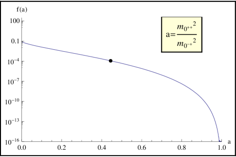
Figure 3: Kinematic suppression factor $f(a)$. Point corresponds to a value of $a$ taken for v-glueball masses from the Morningstar and Peardon spectrum [11].

Decays of the $2^{++}$ state.

Decays of the $2^{++}$ glueball to two gauge bosons are induced by more than one operator in (9). In particular, the $2^{++}$ decays due to the $T_{\mu\nu}$ and $L_{\mu\nu\alpha\beta}$ operators. This corresponds to the amplitude

$$\frac{\alpha_{i}\alpha_{v}}{M^{4}}\,\chi_{i}\left[C_{T}\langle G^{a},G^{b}|\,{\rm tr\ }{G}_{\mu\alpha}{G}_{\nu}^{~{}\alpha}|\,0\rangle\,\langle 0|\,T^{\mu\nu}|2^{++}\rangle+\right.\\ \left.+C_{L}\langle G^{a},G^{b}|\,{\rm tr\ }{G}_{\mu\nu}{G}_{\alpha\beta}|\,0\rangle\langle 0|\,L^{\mu\nu\alpha\beta}|2^{++}\rangle\right].$$ (29)

The width of the decay to two gluons is

$$\begin{array}[]{c}\displaystyle\Gamma_{2^{+}\rightarrow gg}=\frac{\alpha_{s}^{2}\alpha_{v}^{2}(N_{c}^{2}-1)}{160\pi M^{8}}\,\chi_{s}^{2}m_{2^{+}}^{3}\left(\frac{1}{2}\,C_{T}^{2}({\bf F_{2^{++}}^{T}})^{2}+\frac{4}{3}\,C_{L}^{2}({\bf F_{2^{++}}^{L}})^{2}\right).\end{array}$$ (30)

Here we used the following expressions for the matrix elements:

$$\begin{array}[]{c}\displaystyle\langle 0|T^{\mu\nu}|2^{++}\rangle={\bf F_{2^{++}}^{T}}\,\epsilon^{\mu\nu},\end{array}$$ (31)

$$\begin{array}[]{c}\displaystyle\langle 0|L^{\mu\nu\alpha\beta}|2^{++}\rangle={\bf F_{2^{++}}^{L}}\left[{\mathcal{P}}_{\mu\alpha}\epsilon_{\nu\beta}-{\mathcal{P}}_{\mu\beta}\epsilon_{\nu\alpha}+{\mathcal{P}}_{\nu\beta}\epsilon_{\mu\alpha}-{\mathcal{P}}_{\nu\alpha}\epsilon_{\mu\beta}\right],\end{array}$$ (32)

where ${\mathcal{P}}_{\alpha\beta}$ is defined in the caption to table 4.

The branching fraction for the decay to two photons is again similar to (18). For two Z bosons in the final state, the width of the decay is equal to

$$\Gamma_{2^{+}\to ZZ}=\frac{\alpha_{w}^{2}\alpha_{v}^{2}}{40\pi M^{8}}\,\chi_{Z}^{2}{m_{2^{+}}^{3}}(1-4\zeta_{2})^{1/2}\left(\frac{1}{2}\,C_{T}^{2}f_{T}(\zeta_{2})({\bf F_{2^{++}}^{T}})^{2}+\right.\\ \left.\frac{4}{3}\,C_{L}^{2}f_{L}(\zeta_{2})({\bf F_{2^{++}}^{L}})^{2}+\frac{40}{3}\,C_{T}C_{L}f_{TL}(\zeta_{2}){\bf F_{2^{++}}^{T}}{\bf F_{2^{++}}^{L}}\right),$$ (33)

where $f_{T}$, $f_{L}$, $f_{TL}$ are the following functions of the parameter $\zeta_{2}=m_{Z}^{2}/m_{2^{+}}^{2}$.

$$\begin{array}[]{c}\displaystyle f_{T}(\zeta_{2})=1-3\zeta_{2}+6\zeta_{2}^{2}\ ,\ f_{L}(\zeta_{2})=1+2\zeta_{2}+36\zeta_{2}^{2}\ ,\ f_{TL}(\zeta_{2})=\zeta_{2}(1-\zeta_{2})\ .\end{array}$$ (34)

The decay to $W^{+}W^{-}$ is obtained from Eq. (33) by substituting $\chi_{Z}\to\chi_{W}$, $m_{Z}\to m_{W}$ and multiplying by $1/2$. For the $\gamma Z$ final state, the decay rate is

$$\Gamma_{2^{+}\to\gamma Z}=\frac{\alpha\alpha_{w}\alpha_{v}^{2}}{80\pi M^{8}}\,\chi_{\gamma Z}^{2}{m_{2^{+}}^{3}}(1-\zeta_{2})^{3}\left(\frac{1}{2}\,C_{T}^{2}g_{T}(\zeta_{2})({\bf F_{2^{++}}^{T}})^{2}+\right.\\ \left.\frac{4}{3}\,C_{L}^{2}g_{L}(\zeta_{2})({\bf F_{2^{++}}^{L}})^{2}+\frac{20}{3}\,C_{T}C_{L}\zeta_{2}{\bf F_{2^{++}}^{T}}{\bf F_{2^{++}}^{L}}\right),$$ (35)

where

$$\begin{array}[]{c}\displaystyle g_{T}(\zeta_{2})=1+\frac{1}{2}\,\zeta_{2}+\frac{1}{6}\,\zeta_{2}^{2},\qquad g_{L}(\zeta_{2})=1+3\zeta_{2}+6\zeta_{2}^{2}.\end{array}$$ (36)

As in the case of the $0^{-+}$, we can ignore the three-body transitions $2^{++}\to 0^{++}+gg$, etc.

Decays of the $2^{-+}$ state.

The dominant decays of the $2^{-+}$ state occur due to the $L_{\mu\nu\alpha\beta}$ operator. The amplitude for such decays is given by

$$\frac{\alpha_{i}\alpha_{v}}{M^{4}}\,\chi_{i}C_{L}\langle G^{a},G^{b}|\,{\rm tr\ }{G}_{\mu\nu}{G}_{\alpha\beta}|\,0\rangle\langle 0|\,L^{\mu\nu\alpha\beta}|\,2^{-+}\rangle.$$ (37)

The correct Lorentz structure that singles out the negative parity part of the operator $L_{\mu\nu\alpha\beta}$ is as follows:

$$\langle 0|L^{\mu\nu\alpha\beta}|\,2^{-+}\rangle={\bf F_{2^{-+}}^{L}}\left(\epsilon_{\mu\nu\rho\sigma}\epsilon^{\sigma}_{~{}\beta}n^{\rho}n_{\alpha}-\epsilon_{\mu\nu\rho\sigma}\epsilon^{\sigma}_{~{}\alpha}n^{\rho}n_{\beta}+\right.\\ \left.+\epsilon_{\alpha\beta\rho\sigma}\epsilon^{\sigma}_{~{}\nu}n^{\rho}n_{\mu}-\epsilon_{\alpha\beta\rho\sigma}\epsilon^{\sigma}_{~{}\mu}n^{\rho}n_{\nu}\right),$$ (38)

where $n_{\mu}=p^{\,\mu}/m_{2^{-}}$ is a unit vector in the direction of the 4-momentum of the v-glueball.

The decay rate to two gluons is then given by

$$\begin{array}[]{c}\displaystyle\Gamma_{2^{-}\to gg}=\frac{\alpha_{s}^{2}\alpha_{v}^{2}}{120\pi M^{8}}\,(N_{c}^{2}-1){\chi_{s}}^{2}m_{2^{-}}^{3}C_{L}^{2}({\bf F_{2^{-+}}^{L}})^{2}\end{array}$$ (39)

and $\Gamma_{2^{-}\to\gamma\gamma}$ is provided by the same relation as (18). The widths of the decay to $ZZ$ and $\gamma Z$ can be found from the ratios

$$\begin{array}[]{c}\displaystyle\frac{\Gamma_{2^{-}\to ZZ}}{\Gamma_{2^{-}\to gg}}=\frac{1}{2}\,\frac{\alpha_{w}^{2}}{\alpha_{s}^{2}}\frac{\chi_{Z}^{2}}{\chi_{s}^{2}}\,\left(1-4\frac{m_{Z}^{2}}{m_{2^{-}}^{2}}\right)^{1/2}\left(1+2\frac{m_{Z}^{2}}{m_{2^{-}}^{2}}-24\frac{m_{Z}^{4}}{m_{2^{-}}^{4}}\right)\ ,\end{array}$$ (40)

$$\begin{array}[]{c}\displaystyle\frac{\Gamma_{2^{-}\to\gamma Z}}{\Gamma_{2^{-}\to gg}}=\frac{1}{4}\,\frac{\alpha\alpha_{w}}{\alpha_{s}^{2}}\frac{\chi_{\gamma Z}^{2}}{\chi_{s}^{2}}\,\left(1-\frac{m_{Z}^{2}}{m_{2^{-}}^{2}}\right)^{3}\left(1+3\frac{m_{Z}^{2}}{m_{2^{-}}^{2}}+6\frac{m_{Z}^{4}}{m_{2^{-}}^{4}}\right)\ ,\end{array}$$ (41)

and the width for the decay to $W^{+}W^{-}$ is again obtained by substituting in (40) $\chi_{Z}\to\chi_{W}$, $m_{Z}\to m_{W}$ and dividing the result by 2.

As before, we can neglect 3-body decays. However, there is a 2-body radiative decay that we should consider, although, as we will see, for the masses in figure 1 it is of the same order as the 3-body decays. For the $SU(3)$ spectrum in [11] (and possibly all pure glue $SU(n)$, $n\geq 3$) the $2^{-+}$ state is slightly heavier than the lightest state in the $C$-odd sector, the pseudovector $1^{+-}$. Thus, we need at least to consider the decay $2^{-+}\to 1^{+-}+\gamma$. This decay is induced by the second type of operators (table 3) in the effective action (9). The amplitude of the decay reads

$$\begin{array}[]{c}\displaystyle\frac{eg_{v}^{3}}{(4\pi)^{2}M^{4}}\,\chi\langle\gamma|\,G^{\mu\nu}|\,0\rangle\,\left(C_{\Omega^{(1)}}\langle 1^{+-}|\,\Omega_{\mu\nu}^{(1)}|\,2^{-+}\rangle+C_{\Omega^{(2)}}\langle 1^{+-}|\,\Omega_{\mu\nu}^{(2)}|\,2^{-+}\rangle\right)\ .\end{array}$$ (42)

Unfortunately nothing quantitative is known about matrix elements like $\langle 1^{+-}|\Omega_{\mu\nu}^{(n)}|\,2^{-+}\rangle$. In fact each contains multiple Lorentz structures, constructed out of polarization tensors $\epsilon_{\alpha}$, $\epsilon_{\beta\gamma}$ and momenta $p$ and $q$ of the $1^{+-}$ and $2^{-+}$ v-glueballs, times functions of the momentum transfer, cf. [28]. Some simplification can be made if one takes into account the fact that masses of the v-glueballs are close, which we will assume below.

We start by writing the general expression for the amplitude (42):

$$\langle\,\gamma|\,G^{\mu\nu}|\,0\rangle\,\langle\,1^{+-}|\,\Omega_{\mu\nu}^{(n)}|\,2^{-+}\rangle=2{\bf M_{2^{-+}1^{+-}}^{\Omega^{(n)}}}(k\cdot p\,\varepsilon^{\alpha}\epsilon_{\alpha\beta}\epsilon^{\beta}-p\cdot\varepsilon\,k^{\alpha}\epsilon_{\alpha\beta}\epsilon^{\beta})+\\ +2{\bf M_{2^{-+}1^{+-}}^{\Omega^{(n)}\prime}}(k\cdot p\,\varepsilon\cdot\epsilon-k\cdot\epsilon p\cdot\varepsilon)\,\frac{p^{\alpha}\epsilon_{\alpha\beta}p^{\beta}}{m_{2^{-}}^{2}}+\\ +2{\bf M_{2^{-+}1^{+-}}^{\Omega^{(n)}\prime\prime}}(k\cdot p\,\varepsilon^{\alpha}\epsilon_{\alpha\beta}p^{\beta}-p\cdot\varepsilon\,k^{\alpha}\epsilon_{\alpha\beta}p^{\beta})\frac{q\cdot\epsilon}{m_{2^{-}}^{2}}\,,$$ (43)

where $n=1,2$ and $k$, $\varepsilon_{\alpha}$ are the momentum and polarization of the photon. All contributions of the terms proportional to primed form-factors (which correspond to higher partial waves) are suppressed by powers of $(m_{2^{-}}-m_{1^{+}})/(m_{2^{-}}+m_{1^{+}})\simeq 0.017$, so we may neglect them. Note, however, that if the mass splitting is much larger for $n_{v}>3$, then there will be additional unknown quantities that will modify our result below.

We now find

$$\Gamma_{2^{-}\to 1^{+}+\gamma}=\frac{\alpha\alpha_{v}^{3}}{960\pi M^{8}}\,{\chi^{2}}\,\frac{(m_{2^{-}}^{2}-m_{1^{+}}^{2})^{3}}{m_{2^{-}}^{5}m_{1^{+}}^{2}}\,\times\\ \times(3m_{2^{-}}^{4}+34m_{2^{-}}^{2}m_{1^{+}}^{2}+3m_{1^{+}}^{4})\left({\bf M_{2^{-+}1^{+-}}^{\Omega}}\right)^{2}.$$ (44)

Here we introduced the notation

$$\begin{array}[]{c}\displaystyle{\bf M_{2^{-+}1^{+-}}^{\Omega}}\equiv C_{\Omega^{(1)}}{\bf M_{2^{-+}1^{+-}}^{\Omega^{(1)}}}+C_{\Omega^{(2)}}{\bf M_{2^{-+}1^{+-}}^{\Omega^{(2)}}}.\end{array}$$ (45)

Since the the form-factors ${\bf M_{2^{-+}1^{+-}}^{\Omega^{(n)}}}$ are unknown, we shall not distinguish between them and will use a collective notation, similar to (45), for them in the future. In the same manner we will use the notation

$$\begin{array}[]{c}\displaystyle\Omega_{\mu\nu}\equiv C_{\Omega^{(1)}}\Omega^{(1)}_{\mu\nu}+C_{\Omega^{(2)}}\Omega^{(2)}_{\mu\nu}.\end{array}$$ (46)

The factor $(m_{2^{-}}^{2}-m_{1^{+}}^{2})^{3}$ strongly suppresses the amplitude, given the spectrum of figure 1, and a rough estimate suggests it is of the same size as the three-body decays of the $2^{-}$ state, and consequently negligible. However this splitting is so small that it is sensitive to numerical uncertainties in the lattice calculation, and might well be different for other gauge groups. In particular, this decay channel might be closed, or might be more widely open than suggested by figure 1, depending on the mass spectrum.

Given the uncertainty on the spectrum and the unknown v-glueball mass scale, it is worth noting that the radiative decay of $2^{-+}$ to $1^{+-}$ can in principle occur through an emission of the $Z$ boson. This decay is slightly more involved than the decay with photon emission considered above. Additional unknown form factors related to the finiteness of the $Z$ mass further reduce the predictive power of any computation. But such a decay may be forbidden by kinematics, and if allowed it is probably of little importance for the discovery of v-glueballs. Its rate will almost certainly lie somewhere between 0 and $\tan^{2}\theta_{W}\sim 20$% of the rate for decays to a photon. There is no reason for the form factors ${\bf M}(k^{2})$ to be enhanced at $k^{2}\simeq m_{Z}^{2}$. Since the $Z$ boson has only a few percent branching fraction to electrons and muons, the ratio of identifiable $Z$ decays to photon decays is less than 2%. We therefore will not present formulas for this decay mode.

Again we emphasize that in obtaining the results (44) we made some assumptions and approximations, including $\Delta m\ll m_{2^{-}}$, and these results may require generalization in other calculations. However, we will adhere to similar simplifying approximations in the other radiative decays computed below.

4.2 Decays of the vector and pseudovector

In the $C$-odd sector, the lightest v-glueballs are the pseudovector $1^{+-}$ and vector $1^{--}$. The lowest-dimension operators that can create or destroy $1^{--}$ and $1^{+-}$ v-glueballs are the $d=6$ $\Omega_{\mu\nu}$ operators (table 3). Direct annihilation to non-abelian SM gauge bosons would require an operator in the effective action of dimension $D=12$, and is hence negligible. Instead these operators, combined with a hypercharge field strength tensor to form an operator of dimension 8, induce radiative decays to $C$-even v-glueballs, and potentially, for the $1^{--}$ state, annihilation to SM fermions via an off-shell $\gamma$ or $Z$. Three-body decays induced by the dimension 4 operators $S,P,T,L$, although quite uncertain because of the presence of many decay channels with many form factors, appear to be sufficiently suppressed by phase space that they can be disregarded.

Below, we will generally not write formulas for radiative decays by $Z$ emission. As we discussed for the $2^{-}\to 1^{+}+\gamma/Z$ decay, the ratio of leptonic $Z$ bosons to photons is unlikely to reach $2\%$, even if there is no phase space suppression (which there typically is.) Moreover, decays to $Z$ are described by a larger number of unknown form factors, making any attempt to predict the corresponding decay widths and branching ratios even more uncertain than for photon emission.

Decays of the $1^{+-}$ state.

Since the $1^{+-}$ is the lightest v-glueball in the $C$-odd sector, it can only decay, radiatively, to the lighter v-glueballs in the $C$-even sector.

According to table 5, the amplitude of the decay $1^{+-}\rightarrow 0^{++}+\gamma$ is given by

$$\begin{array}[]{c}\displaystyle\frac{eg_{v}^{3}}{(4\pi)^{2}M^{4}}\,{\chi}\langle\,\gamma|\,G^{\mu\nu}|\,0\rangle\,\langle 0^{++}|\,\Omega_{\mu\nu}|\,1^{+-}\rangle=\frac{eg_{v}^{3}\chi}{(4\pi)^{2}M^{4}}\,2k_{\mu}\varepsilon_{\nu}\epsilon^{\mu\nu\alpha\beta}p_{\alpha}\epsilon_{\beta}{\bf M_{1^{+-}0^{++}}^{\Omega}},\end{array}$$ (47)

where $\varepsilon_{\mu}$ and $\epsilon_{\mu}$ are the polarization vectors of the photon and the pseudovector v-glueball respectively; $p_{\mu}$ is the 4-momentum of the $0^{++}$. The Levi-Civita tensor assures the final particles are in a p-wave, as required by parity conservation. The decay rate of this process is

$$\begin{array}[]{c}\displaystyle\Gamma_{1^{+}\to 0^{+}+\gamma}=\frac{\alpha\alpha_{v}^{3}}{24\pi M^{8}}\,{\chi^{2}}\,\frac{(m_{1^{+}}^{2}-m_{0^{+}}^{2})^{3}}{m_{1^{+}}^{3}}\,({\bf M_{1^{+-}0^{++}}^{\Omega}})^{2}.\end{array}$$ (48)

In the case of the decay to the pseudoscalar v-glueball $1^{+-}\rightarrow 0^{-+}+\gamma$, the amplitude is given by

$$\frac{eg_{v}^{3}}{(4\pi)^{2}M^{4}}\,\chi\langle\,\gamma|\,G^{\mu\nu}|\,0\rangle\,\langle 0^{-+}|\,\Omega_{\mu\nu}|\,1^{+-}\rangle=\\ =\frac{eg_{v}^{3}}{(4\pi)^{2}M^{4}}\,\chi\ 2k^{\mu}\varepsilon^{\nu}(p_{\mu}\epsilon_{\nu}-p_{\nu}\epsilon_{\mu}){\bf M_{1^{+-}0^{-+}}^{\Omega}},$$ (49)

where $p_{\mu}$ is the 4-momentum of the $0^{-+}$. The rate of the decay to the pseudoscalar is then

$$\begin{array}[]{c}\displaystyle\Gamma_{1^{+}\to 0^{-}+\gamma}=\frac{\alpha\alpha_{v}^{3}}{24\pi M^{8}}\,{\chi^{2}}\,\frac{(m_{1^{+}}^{2}-m_{0^{-}}^{2})^{3}}{m_{1^{+}}^{3}}\,({\bf M_{1^{+-}0^{-+}}^{\Omega}})^{2}.\end{array}$$ (50)

The ratio of the decay rates to $0^{-+}$ and $0^{++}$ is

$$\begin{array}[]{c}\displaystyle\frac{\Gamma_{1^{+}\rightarrow 0^{-}+\gamma}}{\Gamma_{1^{+}\rightarrow 0^{+}+\gamma}}=\left(\frac{m_{1^{+}}^{2}-m_{0^{-}}^{2}}{m_{1^{+}}^{2}-m_{0^{+}}^{2}}\right)^{3}\left(\frac{{\bf M_{1^{+-}0^{-+}}^{\Omega}}}{{\bf M_{1^{+-}0^{++}}^{\Omega}}}\right)^{2}.\end{array}$$ (51)

For the spectrum of figure 1, the factor involving the masses is about 0.39; the ratio of matrix elements is unknown, but if we guess that ${{\bf M_{1^{--}0^{\pm+}}^{\Omega}}}\sim 1/{\bf F^{S,P}_{0^{\pm+}}}$, as would be true for pion emission, and use the lattice results from [17], we would find this ratio to be slightly larger than 1. In any case, there is no sign of a significant suppression of one rate relative to the other.

Finally, in the case of the decay to the tensor v-glueball, the amplitude $1^{+-}\rightarrow 2^{++}+\gamma$ contains two independent form factors in the lowest partial wave approximation, denoted ${\bf M_{1^{+-}0^{-+}}^{\Omega}}$ and ${\bf{M^{\prime}}_{1^{+-}0^{-+}}^{\Omega}}$,

$$\frac{eg_{v}^{3}}{(4\pi)^{2}M^{4}}\,\chi\langle\,\gamma|\,G^{\mu\nu}|\,0\rangle\,\langle 2^{++}|\,\Omega_{\mu\nu}|\,1^{+-}\rangle=\\ =\frac{eg_{v}^{3}}{(4\pi)^{2}M^{4}}\,\chi\ 2k^{\mu}\varepsilon^{\nu}\epsilon_{\mu\nu\alpha\beta}\epsilon_{\beta\lambda}(\epsilon_{\lambda}p_{\alpha}{\bf M_{1^{+-}0^{-+}}^{\Omega}}+\epsilon_{\alpha}p_{\lambda}{\bf{M^{\prime}}_{1^{+-}0^{-+}}^{\Omega}})$$ (52)

and the corresponding decay rate is

$$\Gamma_{1^{+}\to 2^{+}+\gamma}=\frac{\alpha\alpha_{v}^{3}}{576\pi M^{8}}\,{\chi^{2}}\,\frac{(m_{1^{+}}^{2}-m_{2^{+}}^{2})^{3}}{m_{1^{+}}^{5}m_{2^{+}}^{2}}\,\left(3m_{2^{+}}^{4}+34m_{1^{+}}^{2}m_{2^{+}}^{2}+3m_{1^{+}}^{4}\right)\times\\ \times\left[\left({\bf M_{1^{+-}2^{++}}^{\Omega}}+{\bf{M^{\prime}}_{1^{+-}2^{++}}^{\Omega}}f(m_{1^{+}},m_{2^{+}})\right)^{2}\right.\\ \left.+\left({\bf{M^{\prime}}_{1^{+-}2^{++}}^{\Omega}}\right)^{2}g(m_{1^{+}},m_{2^{+}})\right],$$ (53)

where $f$ and $g$ are the following functions of the v-glueball masses,

$$\begin{array}[]{c}\displaystyle f(m_{1^{+}},m_{2^{+}})=\frac{\left(m_{2^{+}}^{2}-m_{1^{+}}^{2}\right)\left(3m_{2^{+}}^{2}+7m_{1^{+}}^{2}\right)}{3m_{2^{+}}^{4}+34m_{1^{+}}^{2}m_{2^{+}}^{2}+3m_{1^{+}}^{4}},\end{array}$$ (54)

$$\begin{array}[]{c}\displaystyle g(m_{1^{+}},m_{2^{+}})=12\,\frac{\left(m_{2^{+}}^{2}-m_{1^{+}}^{2}\right)^{2}m_{1^{+}}^{2}(6m_{2^{+}}^{4}+8m_{1^{+}}^{2}m_{2^{+}}^{2}+m_{1^{+}}^{4})}{m_{2^{+}}^{2}\left(3m_{2^{+}}^{4}+34m_{1^{+}}^{2}m_{2^{+}}^{2}+3m_{1^{+}}^{4}\right)^{2}}.\end{array}$$ (55)

Decays of the $1^{--}$ state.

The decays of the vector v-glueball are similar to the decays of the pseudovector, with a few additions. In contrast to the case of the $1^{+-}$, the $1^{--}$ can annihilate through an off-shell vector boson to a SM fermion-antifermion pair. But the radiative decays to light v-glueballs in the $C$-even sector still typically dominate.

The radiative decay to the scalar, $1^{--}\to 0^{++}+\gamma$, is analogous to the decay $1^{--}\to 0^{++}+\gamma$; see table 5 and (50). Thus, its rate is

$$\begin{array}[]{c}\displaystyle\Gamma_{1^{-}\to 0^{+}+\gamma}=\frac{\alpha\alpha_{v}^{3}}{24\pi M^{8}}\,{\chi^{2}}\,\frac{(m_{1^{-}}^{2}-m_{0^{+}}^{2})^{3}}{m_{1^{-}}^{3}}\,({\bf M_{1^{--}0^{++}}^{\Omega}})^{2}.\end{array}$$ (56)

The decay to the pseudoscalar is analogous to the decay (48) and has the rate

$$\begin{array}[]{c}\displaystyle\Gamma_{1^{-}\to 0^{-}+\gamma}=\frac{\alpha\alpha_{v}^{3}}{24\pi M^{8}}\,{\chi^{2}}\,\frac{(m_{1^{-}}^{2}-m_{0^{-}}^{2})^{3}}{m_{1^{-}}^{3}}\,({\bf M_{1^{--}0^{-+}}^{\Omega}})^{2}.\end{array}$$ (57)

The amplitude of the decay to the $2^{++}$ state is similar to the amplitude (43) of the decay $2^{-+}\to 1^{+-}+\gamma$. However, in this case the masses of the two states are not close, and our approximation which allowed us to ignore the contribution of three additional form factors is not valid. We therefore restrict ourselves to just demonstrating the general expression for the amplitude.

$$\frac{eg_{v}^{3}\chi}{(4\pi)^{2}M^{4}}\langle\,\gamma|\,G^{\mu\nu}|\,0\rangle\langle 2^{++}|\,\Omega_{\mu\nu}|\,1^{--}\rangle=2{\bf M_{1^{--}2^{++}}^{\Omega}}(k\cdot p\,\varepsilon^{\alpha}\epsilon_{\alpha\beta}\epsilon^{\beta}-p\cdot\varepsilon\,k^{\alpha}\epsilon_{\alpha\beta}\epsilon^{\beta})\\ +2{\bf M_{1^{--}2^{++}}^{\Omega\prime}}(k\cdot q\,\varepsilon\cdot\epsilon-k\cdot\epsilon q\cdot\varepsilon)\,\frac{q^{\alpha}\epsilon_{\alpha\beta}q^{\beta}}{m_{1^{-}}^{2}}+\\ +2{\bf M_{1^{--}2^{++}}^{\Omega\prime\prime}}(k\cdot q\,\varepsilon^{\alpha}\epsilon_{\alpha\beta}q^{\beta}-q\cdot\varepsilon\,k^{\alpha}\epsilon_{\alpha\beta}q^{\beta})\frac{p\cdot\epsilon}{m_{1^{-}}^{2}}.$$ (58)

A complete formula for the decay rate is not very useful, given the large number of unknown form factors that enter.

The $1^{--}$ state is also massive enough to decay to the $2^{-+}$ state. This decay has an amplitude similar to the decay $1^{+-}\to 2^{++}+\gamma$, given in (52). One can find the decay rate

$$\Gamma_{1^{-}\to 2^{-}+\gamma}=\frac{\alpha\alpha_{v}^{3}}{576\pi M^{8}}\,{\chi^{2}}\,\frac{(m_{1^{-}}^{2}-m_{2^{-}}^{2})^{3}}{m_{1^{-}}^{5}m_{2^{-}}^{2}}\,\left(3m_{2^{-}}^{4}+34m_{1^{-}}^{2}m_{2^{-}}^{2}+3m_{1^{-}}^{4}\right)\times\\ \times\left[\left({\bf M_{1^{--}2^{-+}}^{\Omega}}+{\bf{M^{\prime}}_{1^{--}2^{-+}}^{\Omega}}f(m_{1^{-}},m_{2^{-}})\right)^{2}\right.\\ \left.+\left({\bf{M^{\prime}}_{1^{--}2^{-+}}^{\Omega}}\right)^{2}g(m_{1^{-}},m_{2^{-}})\right],$$ (59)

where functions $f$ and $g$ are defined by (54) and (55) respectively.

Now we consider the decay of the $1^{--}$ to SM fermion pairs through an off-shell $\gamma$ or $Z$. For large $m_{1^{-}}$ we can neglect the $Z$ mass and treat the radiated particle as an off-shell hypercharge boson. The amplitude reads

$$\begin{array}[]{c}\displaystyle\frac{\alpha g^{3}_{v}}{2\pi M^{4}}\,\frac{\chi}{\cos^{2}\theta_{W}}\,\langle f,\bar{f}|Y_{L}\bar{\psi}_{L}\gamma^{\mu}\psi_{L}+Y_{R}\bar{\psi}_{R}\gamma^{\mu}\psi_{R}|\,0\rangle\,\frac{1}{p^{2}}\,\langle 0|p^{\nu}\Omega_{\nu\mu}|1^{--}\rangle.\end{array}$$ (60)

Here $Y_{L}$ and $Y_{R}$ are left and right hypercharges of the emitted fermions. The matrix element of $\Omega_{\mu\nu}$ can be read off from table 4. The width (ignoring the fermion masses) is given by

$$\begin{array}[]{c}\displaystyle\Gamma_{1^{-}\to\bar{f}f}=\frac{{2\alpha^{2}}\alpha_{v}^{3}}{3M^{8}}\,\frac{\chi^{2}}{\cos^{4}\theta_{W}}\,(Y_{L}^{2}+Y_{R}^{2})\,m_{1^{-}}^{3}({\bf F_{1^{--}}^{\Omega}})^{2}.\end{array}$$ (61)

For quarks a factor of 3 must be included to account for color.

The above result is valid for $m_{1^{-}}\gg m_{Z}$. For smaller $m_{1^{-}}$ one must account for the non-zero $Z$ mass through the substitution

$$\frac{(Y_{L}^{2}+Y_{R}^{2})}{\cos^{4}\theta_{W}}\to\left(Q-\frac{Q\cos^{2}\theta_{W}-Y_{L}}{\cos^{2}\theta_{W}}\,\frac{m_{1^{-}}^{2}}{m_{1^{-}}^{2}-m_{Z}^{2}}\right)^{2}+\\ +Y_{R}^{2}\left(1+\frac{\sin^{2}\theta_{W}}{\cos^{2}\theta_{W}}\,\frac{m_{1^{-}}^{2}}{m_{1^{-}}^{2}-m_{Z}^{2}}\right)^{2},$$ (62)

which accounts for a finite mass of the $Z$-boson. Here $Q=T_{3}+Y$ is the charge of $f$. A quick check shows that this rate, whose ratio to radiative decays is (for large $m_{1^{-}}$)

$$\begin{array}[]{c}\displaystyle\frac{\Gamma_{1^{-}\to\gamma^{*}/Z^{*}\to f\bar{f}}}{\Gamma_{1^{-}\rightarrow 0^{+}+\gamma}}=\frac{16\pi\alpha}{\cos^{4}\theta_{W}}\,(Y_{L}^{2}+Y_{R}^{2})\left(\frac{m_{1^{-}}^{2}}{m_{1^{-}}^{2}-m_{0^{+}}^{2}}\right)^{3}\left(\frac{{\bf F_{1^{--}}^{\Omega}}}{{\bf M_{1^{--}0^{++}}^{\Omega}}}\right)^{2},\end{array}$$ (63)

is not negligible. The first factor in curved brackets is a factor of a few, while the second factor in curved brackets may be large, especially at large $n_{v}$. Decays to electrons and muons will be reconstructable as a resonance, so despite the uncertain branching fractions this decay mode is worthy of careful consideration.

Decay of the $1^{--}$ state to the $1^{+-}$ v-glueball can only proceed with the emission of at least two SM gauge bosons. Although such decays are suppressed, the details of the calculation for $1^{--}\to 1^{+-}+gg$ are presented in the Appendix.

4.3 Decays of the remaining states

We may infer without detailed calculation that the likely decays of the other v-glueballs in the $C$-odd sector are radiative. Three-body decays to two gauge bosons plus another $C$-odd v-glueball are quite suppressed by phase space, because the mass splittings in the $C$-odd sector are never large. Even the splitting of the $0^{+-}$ state from the $1^{+-}$ state is only 1.1 $m_{0^{++}}$. By contrast, two-body radiative decays into the $C$-even sector have significantly larger phase space. (In the appendix, we confirm this for decays of the $1^{--}$ state.) Meanwhile, no operator appearing in the effective action at dimension $D=8$ permits the $0^{+-}$, $2^{\pm-}$, or $3^{\pm-}$ states to annihilate directly to standard model particles. Therefore, we should expect that all of these states decay radiatively, emitting typically a photon or more rarely (if kinematically allowed) a $Z$, to a v-glueball of opposite $C$. Their lifetimes will be of order or slightly shorter than that of the $1^{-+}$, due to enhanced phase space and additional decay channels.

The $3^{++}$ state is more complicated. No operator allows it to annihilate directly to standard model gauge bosons, so it will decay either by a two-body radiative transition to the $C$-odd sector or by a three-body decay to two gauge bosons plus a $C$-even v-glueball. For this state, in contrast to the $C$-odd states, the mass splittings tend to suppress the radiative decay and enhance the three-body decays. With many contributing decay channels and unknown form factors, it seems impossible to estimate which type of decay is dominant. Indeed simple estimates suggest they are of the same order, with large uncertainties. Qualitatively, if the colored $X$ particles are very heavy and $\chi_{s}$ is very small, radiative decays will probably dominate, while tight degeneracies within the $X$ multiplet(s) could suppress $\chi$ and reverse the situation. But quantitative prediction seems impossible.

5 Conclusions

Let us first summarize our results and their immediate implications.

• We have seen that annihilation decays dominate those states that can be created by dimension $d=4$ operators (the $0^{\pm+}$ and $2^{\pm+}$). Their branching fractions are dominated by decays to $gg$, with decays to $\gamma\gamma$ having a branching fraction of $\sim 0.4\%$, assuming the $X$ fields form complete $SU(5)$ multiplets of equal mass. If the colored $X$ particles are much heavier than the uncolored ones, then decays to electroweak bosons can dominate.

• Most other states decay by radiatively emitting a photon, or (at a rate that is at most $\tan^{2}\theta_{W}$ compared to photon emission) a $Z$ boson.

• The $1^{--}$ is a special case; it typically prefers to decay radiatively but has a non-negligible annihilation decay to an off-shell $\gamma$ or $Z$.

• The $3^{++}$ is also special; three-body decays to gluons plus a $C$-even v-glueball could be of the same order or even dominate over radiative decays to the $C$-odd sector.

• In all, we expect the final states from v-glueball production to be rich in jets and stray photons, with occasional photon pairs, leptons and some missing energy from neutrinos. The two-photon resonances from the annihilation decays of $C$-even v-glueballs are likely to be the discovery signatures, along with the $\gamma\gamma\gamma$ and $\gamma gg$ resonances from cascade decays of $C$-odd v-glueballs.

• Depending on the parameters, the lifetime of any given state can vary over many orders of magnitude. But for any fixed choice of parameters, lifetimes of the v-glueballs vary over at least three or four orders of magnitude, the details depending on unknown v-glueball matrix elements and mass ratios, as well as the $X$ mass spectrum. Displaced vertices can potentially serve as a discovery channel.

• There are several opportunities for discovery of this signal in displaced vertices. One option arises from $gg$ decays in events triggered by photons, another from $W^{+}W^{-}$ decays triggered by the muon or electron in a leptonic $W$ decay, and a third from photons that arrive late or (if converted) point away from the primary vertex.

Our results are robust, but some cautionary and clarifying remarks are in order. Clearly, numerical application of our formulas is currently subject to considerable uncertainties, due especially to the many unknown matrix elements that arise, and due also to the unknown spectrum for gauge groups other than $SU(3)$. Of course these uncertainties are largely reducible through additional lattice gauge theory computations, should a discovery of a sector of this type be made. However, there are other potential subtleties to keep in mind. If the $X$ fields and the v-glueball states have comparable masses, then mixing between these states cannot be neglected. This could lead to additional physical effects that we have not considered. We also remind the reader that we have worked at leading non-vanishing order and that higher-order corrections are not negligible when precise predictions are required.

A more qualitative uncertainty, and an interesting opportunity, arises from the gauge group. For $SU(n)$, $n>2$, it is anticipated that the glueball spectrum is similar to that of $SU(3)$, as calculated by [11]. However the $SU(2)$ spectrum, and more generally that of any $Sp(2n_{v})$ or $SO(2n_{v}+1)$ gauge group, has no $C$-odd sector. The operators $\Omega_{\mu\nu}^{(i)}$ do not exist, as they are built from the $d^{abc}$ symbol absent from such groups, and the corresponding $C$-odd states are also absent.

For $SO(2n_{v})$ the situation is more subtle. The first cases are $SO(4)$, which is not simple and has two sets of $SU(2)$ v-glueballs, and $SO(6)$, which is the same as $SU(4)$. The $d=6$ $\Omega_{\mu\nu}^{(i)}$ operators are present for $SO(6)$, but for general $SO(2n_{v})$ the $\Omega_{\mu\nu}^{(i)}$ operators become Pfaffian operators of dimension $2n_{v}$, built from a single epsilon symbol and $n_{v}$ field strengths. As suggested by [16] and as verified by [11], there is a correlation in the QCD spectrum and in the glueball spectrum between the dimension of an operator and the mass of the lightest corresponding state. For this reason we expect that for a pure $SO(2n_{v})$ gauge theory with $n_{v}>3$, the $C$-odd states are heavier than in figure 1 relative to the $C$-even states. Their production rate is likely to be quite suppressed as a result, but are still interesting, since several are likely to be unable to decay to other v-glueballs alone, and will be metastable. Certainly the lightest $C$-odd state (probably still the $1^{+-}$) cannot decay to two or more $C$-even v-glueballs, so it will likely decay by radiating a photon or $Z$. Moreover, the degeneracy of the light $C$-odd states seen in $SU(3)$ may well persist more generally, making these states potentially unable to decay to two v-glueballs in a $C$-odd final state, such as $1^{+-}+0^{++}$. All of these states will decay therefore to the $C$-even sector by radiating a photon (or $Z$), except the $1^{--}$ that may again decay to standard model fermions. The larger phase space for $n_{v}>3$ means the lifetimes may be much shorter than those of the $C$-even states, a fact which could be phenomenologically important if $\Lambda_{v}$ and $\Lambda_{v}/M$ are so small that the $C$-even states are unobservably long-lived.

Thus study of the spectrum of the v-glueballs may provide some information on the gauge group. Combined with some partial information about the $X$ production rate and the branching fractions of $X\bar{X}$ annihilations, it may well be possible to identify the gauge group precisely.

Finally, we have assumed here that the v-glueballs are the low-energy degrees of freedom of an asymptotically weakly-coupled gauge theory. The AdS/CFT correspondence [32, 33] allows us to learn what one might observe if the theory has a large ’t Hooft coupling in the ultraviolet. In particular, the low-lying glueballs of such a theory can be described as modes of a string theory on a 10-dimensional space compactified to 5 dimensions. Such a theory [34, 35, 36] will have light scalars, pseudoscalars, tensors, etc., but will not have any light $2^{-+}$ state. Apparently the mass of this state may serve as a crude probe of the size of the ultraviolet ’t Hooft coupling, as long as its mass is not so high as to render the state unstable to decay to lighter glueballs.

Our formulas now permit a variety of phenomenological studies. The issue of LHC searches will be considered in [15].

Appendix

In the main body of the text we have argued that three-body decays of states in the $C$-odd sector are largely suppressed as compared to their radiative decays to light $C$-even states. As an example, here we consider a three-body decay $1^{--}\to 1^{+-}gg$ and demonstrate that there is a substantial suppression of its rate. We will restrict ourselves to consider the case of the s-wave decay mode since this is expected to give the highest contribution to the decay rate in a partial wave expansion. In this approximation only $P$ and $L_{\mu\nu\alpha\beta}$ operators contribute (table 2). This corresponds to the amplitude

$$\frac{\alpha_{s}\alpha_{v}}{M^{4}}\,\chi_{s}\left[C_{P}\langle g^{a},g^{b}|\,{\rm tr\ }{G}_{\mu\nu}{\tilde{G}}^{\mu\nu}|\,0\rangle\,\langle 1^{+-}|\,P|1^{--}\rangle\ +\right.\\ \left.+C_{L}\langle g^{a},g^{b}|\,{\rm tr\ }{G}_{\mu\nu}{G}_{\alpha\beta}|\,0\rangle\langle 1^{+-}|\,L^{\mu\nu\alpha\beta}|1^{--}\rangle\right],$$

where the s-wave approximation implies the following form of the matrix elements;

$$\begin{array}[]{c}\displaystyle\langle 1^{+-}|\,P|1^{--}\rangle=\frac{\epsilon^{+}\cdot\epsilon^{-}}{m_{1^{-}}}\,{\bf M_{1^{--}1^{+-}}^{P}},\end{array}$$

$$\langle 1^{+-},q|\,L_{\mu\nu\alpha\beta}|1^{--},p\rangle=\frac{\bf M_{1^{--}1^{+-}}^{L}}{m_{1^{-}}^{3}}\,(\epsilon_{\mu\nu\rho\sigma}p^{\rho}{\epsilon^{-}}^{\sigma}(p_{\alpha}{\epsilon^{+}}_{\beta}-p_{\beta}{\epsilon^{+}}_{\alpha})+\\ +\epsilon_{\alpha\beta\rho\sigma}p^{\rho}{\epsilon^{-}}^{\sigma}(p_{\mu}{\epsilon^{+}}_{\nu}-p_{\nu}{\epsilon^{+}}_{\mu})-{\rm traces})+\ldots\ ,$$

The above amplitude gives a decay rate

$$\Gamma_{1^{-}\to 1^{+}gg}=\frac{\alpha_{s}^{2}\alpha_{v}^{2}}{2^{9}\pi^{3}M^{8}}\frac{1}{3}(N_{c}^{2}-1)\chi_{s}^{2}m_{1^{-}}^{3}\left(4C_{L}^{2}({\bf M_{1^{--}1^{+-}}^{L}})^{2}\,f_{L}(a)+\right.\\ \left.+C_{P}^{2}({\bf M_{1^{--}1^{+-}}^{P}})^{2}\,f_{P}(a)\right)+\ldots\ ,$$ (64)

where we define the dimensionless functions $f_{L}(a)$ and $f_{P}(a)$ of $a\equiv m_{1^{+}}^{2}/m_{1^{-}}^{2}$ as

$$f_{L}(a)=-\frac{1}{15120a}(171a^{7}-1295a^{6}+4410a^{5}-9450a^{4}+11025a^{3}-\\ -4221a^{2}-630a-10)-\frac{1}{36}\,a(5a-9)\log(a),$$

$$f_{P}(a)=-\frac{1}{120a}\left(a^{6}+36a^{5}+1305a^{4}-1305a^{2}-36a-1\right)+\\ +\frac{1}{2}\,a\left(9a^{2}+28a+9\right)\log(a).$$

For the values of v-glueball masses from the spectrum in figure 1, $a\simeq 0.6$, $f_{L}(0.6)\simeq 3\times 10^{-5}$ and $f_{P}(0.6)\simeq 7\times 10^{-5}$.

The ratio of the decay rate (64) to the radiative two-body decay (56) is

$$\begin{array}[]{c}\displaystyle\frac{\Gamma_{1^{-}\to 1^{+}gg}}{\Gamma_{1^{-}\to 0^{+}\gamma}}=6\times 10^{-6}\frac{\alpha_{s}^{2}}{\alpha\alpha_{v}}\,\frac{\chi_{s}^{2}}{\chi^{2}}\,\left(\frac{4C_{L}^{2}({\bf M_{1^{--}1^{+-}}^{L}})^{2}+\frac{f_{P}}{f_{L}}C_{P}^{2}({\bf M_{1^{--}1^{+-}}^{L}})^{2}}{(\bf M_{1^{--}0^{++}}^{\Omega})^{2}}\right).\end{array}$$

Unless there is an extreme degeneracy in the $SU(5)$ multiplet of $X$ particles, which is unnatural due to $SU(5)$-asymmetric renormalization of the masses, we expect $\chi$ is at least of order $0.1$, so the coefficient in front of the ratio of the form-factors will be around $10^{-2}$ or smaller.

For other states in the $C$-odd sector, a rough estimate confirms that the ratio of the three-body decays to the radiative decays is never greater than $1/10$ and is typically much smaller. Thus, we conclude that the three-body decays in this sector are never dominant. Since most such decays are to gluons, and are therefore very difficult to observe, the three-body processes can for current purposes be ignored.

References

- [1] M. J. Strassler and K. M. Zurek, Phys. Lett. B 651 (2007) 374 [arXiv:hep-ph/0604261].
- [2] M. J. Strassler and K. M. Zurek, Phys. Lett. B 661, 263 (2008) [arXiv:hep-ph/0605193].
- [3] M. J. Strassler, arXiv:hep-ph/0607160.
- [4] M. J. Strassler, arXiv:0801.0629 [hep-ph].
- [5] T. Han, Z. Si, K. M. Zurek and M. J. Strassler, arXiv:0712.2041 [hep-ph].
- [6] M. J. Strassler, arXiv:0806.2385 [hep-ph].
- [7] Z. Chacko, H. S. Goh and R. Harnik, Phys. Rev. Lett. 96, 231802 (2006) [arXiv:hep-ph/0506256].
- [8] G. Burdman, Z. Chacko, H. S. Goh and R. Harnik, JHEP 0702, 009 (2007) [arXiv:hep-ph/0609152].
- [9] K. M. Zurek, arXiv:0811.4429 [hep-ph]; J. March-Russell, S. M. West, D. Cumberbatch and D. Hooper, JHEP 0807 (2008) 058 [arXiv:0801.3440 [hep-ph]]; N. Arkani-Hamed and N. Weiner, JHEP 0812, 104 (2008) [arXiv:0810.0714 [hep-ph]]; A. E. Nelson and C. Spitzer, arXiv:0810.5167 [hep-ph].
- [10] R. Blumenhagen, M. Cvetic, P. Langacker and G. Shiu, Ann. Rev. Nucl. Part. Sci. 55, 71 (2005) [arXiv:hep-th/0502005].
- [11] C. J. Morningstar and M. J. Peardon, Phys. Rev. D 60 (1999) 034509 [arXiv:hep-lat/9901004].
- [12] L. B. Okun, JETP Lett. 31 (1980) 144 [Pisma Zh. Eksp. Teor. Fiz. 31 (1979) 156], Nucl. Phys. B 173 (1980) 1.
- [13] S. Gupta and H. R. Quinn, Phys. Rev. D 25 (1982) 838.
- [14] J. Kang, M. A. Luty and S. Nasri, arXiv:hep-ph/0611322; J. Kang and M. A. Luty, arXiv:0805.4642 [hep-ph].
- [15] J. E. Juknevich, D. Melnikov and M.J. Strassler, in preparation.
- [16] R. L. Jaffe, K. Johnson and Z. Ryzak, Annals Phys. 168 (1986) 344.
- [17] Y. Chen et al., Phys. Rev. D 73 (2006) 014516 [arXiv:hep-lat/0510074].
- [18] V. A. Novikov, L. B. Okun, M. A. Shifman, A. I. Vainshtein, M. B. Voloshin and V. I. Zakharov, Phys. Rept. 41, 1 (1978).
- [19] M. J. Strassler, SLAC-PUB-5978
- [20] S. Groote and A. A. Pivovarov, Eur. Phys. J. C 21, 133 (2001) [arXiv:hep-ph/0103313].
- [21] V. A. Novikov, M. A. Shifman, A. I. Vainshtein and V. I. Zakharov, Nucl. Phys. B 165, 67 (1980).
- [22] V. A. Novikov, M. A. Shifman, A. I. Vainshtein and V. I. Zakharov, Nucl. Phys. B 165, 55 (1980); V. A. Novikov, M. A. Shifman, A. I. Vainshtein and V. I. Zakharov, Phys. Lett. B 86, 347 (1979) [JETP Lett. 29, 594.1979 ZFPRA,29,649 (1979 ZFPRA,29,649-652.1979)].
- [23] J. F. Donoghue, K. Johnson and B. A. Li, Phys. Lett. B 99 (1981) 416.
- [24] J. M. Cornwall and A. Soni, Phys. Lett. B 120 (1983) 431.
- [25] J. Kuti, Nucl. Phys. Proc. Suppl. 73 (1999) 72 [arXiv:hep-lat/9811021]
- [26] M. Loan and Y. Ying, Prog. Theor. Phys. 116, 169 (2006) [arXiv:hep-lat/0603030].
- [27] V. Mathieu, N. Kochelev and V. Vento, arXiv:0810.4453 [hep-ph].
- [28] R. Delbourgo and D. s. Liu, Phys. Rev. D 51, 118 (1995) [arXiv:hep-ph/9403372].
- [29] S. Gao and C. Gale, Phys. Rev. C 57, 254 (1998) [arXiv:nucl-th/9711006].
- [30] R. Rapp and C. Gale, Phys. Rev. C 60, 024903 (1999) [arXiv:hep-ph/9902268].
- [31] N. Kaiser and U. G. Meissner, Nucl. Phys. A 519 (1990) 671.
- [32] J. M. Maldacena, Adv. Theor. Math. Phys. 2, 231 (1998) [Int. J. Theor. Phys. 38, 1113 (1999)] [arXiv:hep-th/9711200]; for a review see O. Aharony, S. S. Gubser, J. M. Maldacena, H. Ooguri and Y. Oz, Phys. Rept. 323, 183 (2000) [arXiv:hep-th/9905111].
- [33] S. S. Gubser, I. R. Klebanov and A. M. Polyakov, Phys. Lett. B 428, 105 (1998) [arXiv:hep-th/9802109]; E. Witten, Adv. Theor. Math. Phys. 2, 253 (1998) [arXiv:hep-th/9802150].
- [34] E. Witten, Adv. Theor. Math. Phys. 2, 505 (1998) [arXiv:hep-th/9803131].
- [35] C. Csaki, H. Ooguri, Y. Oz and J. Terning, JHEP 9901, 017 (1999) [arXiv:hep-th/9806021]; also see R. C. Brower, S. D. Mathur and C. I. Tan, Nucl. Phys. B 587, 249 (2000) [arXiv:hep-th/0003115] and references therein.
- [36] M. Berg, M. Haack and W. Mueck, Nucl. Phys. B 789, 1 (2008) [arXiv:hep-th/0612224]; A. Dymarsky and D. Melnikov, JHEP 0805, 035 (2008) [arXiv:0710.4517 [hep-th]]; M. K. Benna, A. Dymarsky, I. R. Klebanov and A. Solovyov, JHEP 0806, 070 (2008) [arXiv:0712.4404 [hep-th]]; A. Dymarsky, D. Melnikov and A. Solovyov, arXiv:0810.5666 [hep-th].