HISQ action in dynamical simulations

Abstract:

We report on recent progress in employing the Highly Improved Staggered Quark (HISQ) action introduced by the HPQCD/UKQCD collaboration in simulations with dynamical fermions. The HISQ action is an order $a^{2}$ Symanzik-improved action with further suppressed taste symmetry violations. The improvement in taste symmetry is achieved by introducing Fat7 smearing of the original gauge links and reunitarization (projection to an element of U(3) or SU(3)) followed by Asq-type smearing. Major challenges for calculating the fermion force are related to the reunitarization step. We present a preliminary study of the HISQ action on two 2+1+1 flavor ensembles with the lattice spacing roughly equivalent to the MILC asqtad $a=0.125$ and 0.09 fm ensembles.

1 Introduction

The Highly Improved Staggered Quark (HISQ) action developed in Ref. [1] is an $O(a^{2})$ Symanzik-improved action for which additional suppression of taste-exchange interactions is
achieved by replacing the original gauge links $U$ in the Dirac operator by

$$U\rightarrow X={\cal F}_{2}{\cal U}{\cal F}_{1}\,U$$ (1)

where intermediate sets of links $V$, $W$, $X$ are defined as

• ${\cal F}_{1}$ – smearing level 1 (Fat 7): $V={\cal F}_{1}U$,

• ${\cal U}$ – reunitarization: $W={\cal U}V$,

• ${\cal F}_{2}$ – smearing level 2 (Asq): $X={\cal F}_{2}W$.

A new feature of the HISQ action compared with asqtad is the reunitarization step that gives an extra contribution to the fermion force.

2 Fermion force and reunitarization

In molecular dynamics simulations we are sampling an ensemble of gauge configurations weighted by $\exp(-S)$, where the action $S=S_{g}+S_{f}$ is split into gauge, $S_{g}$, and fermionic, $S_{f}$, parts. As usual, the integration over Grassmann variables is performed and then a set of pseudo-fermion fields $\Phi$ is introduced, resulting in the fermionic part of the form $S_{f}\sim\langle\Phi|(M^{\dagger}(U)M(U))^{-N_{f}/4}|\Phi\rangle$. One can consult the details of the algorithm in [2] and recent ideas on efficient evaluation of the fermion force for HISQ in [3].

The fermion force is calculated by taking the derivative of the action $S_{f}$ with respect to fundamental gauge links $U$ using the chain rule along the lines of Refs. [3], [4]. Schematically:

$$\frac{\partial S_{f}}{\partial U}=\frac{\partial S_{f}}{\partial X}\,\frac{\partial X}{\partial W}\,\frac{\partial W}{\partial V}\,\frac{\partial V}{\partial U}\ .$$ (2)

The following parts are the same as for the asqtad action: $\partial S_{f}/\partial X$, $\partial X/\partial W$, $\partial V/\partial U$, while the contribution from the reunitarization step $\partial W/\partial V$ is new.

We have experimented with projecting to SU(3) and U(3) groups and found that pion spectrum measurements with valence HISQ and sea asqtad quarks show no difference, as one would expect on physical grounds. Therefore in our dynamical HISQ simulations we always perform projection to the group U(3). While keeping the physics the same, this has two advantages:

1. Different methods of projection, namely polar decomposition and trace maximization, give identical results. (The same is not true in the SU(3) case.)

2. When projecting from U(3) to SU(3) by making the determinant of the matrix equal to 1, one needs to choose among three possibilities for the phase. In dynamical simulations one needs to track this phase to make sure it changes smoothly for each link. Otherwise discontinuous changes lead to rapid changes in the action similar to those we describe below.

We adopt the following method of U(3) projection. For a complex matrix $V$ the matrix $H=V^{\dagger}V$ is Hermitian and $W=VH^{-1/2}$ is unitary. We first calculate $H^{-1/2}$ by using the Cayley-Hamilton theorem in a manner similar to the approach in Refs. [5], [6]:

$$H^{-1/2}=f_{0}\mathbb{I}+f_{1}H+f_{2}H^{2},$$ (3)

where $f_{i}$ are functions of $c_{i}={\rm Tr}(H^{i+1})/(i+1)$, $i=0,1,2$. To evaluate the derivative of $H^{-1/2}$ with respect to $H$ one needs to know the derivative of $f_{i}$ with respect to $H$. This can be performed analytically by applying the chain rule and making use of the coefficients explicitly calculated in Ref. [6]. After $\partial H^{-1/2}/\partial H$ is known we have trivially:

$$\frac{\partial W}{\partial V}=\frac{\partial V}{\partial V}H^{-1/2}+V\frac{\partial H^{-1/2}}{\partial H}\frac{\partial H}{\partial V}.$$ (4)

(We write Eq. (4) schematically, but in fact each matrix-matrix derivative is a rank 4 tensor with indices contracted in such a way that the resulting expression on the right hand side is a rank 4 tensor again. An excellent review on how to deal with such derivatives can be found in [4].) Thus the entire derivation can be performed analytically. (We also implemented a finite difference scheme and rational function approximation but found them much less accurate than the procedure described here.)

To understand the possible behaviour of $\partial W/\partial V$ qualitatively let us consider the U(1) case for the moment. Then $V=r\,e^{i\theta}$ and $W=V(V^{\dagger}V)^{-1/2}=e^{i\theta}$, and the derivative

$$\frac{\partial W}{\partial V}=\left(\frac{\partial W}{\partial V}\right)_{V^{\dagger}}=\frac{\partial(W,V^{\dagger})}{\partial(V,V^{\dagger})}=\frac{\partial(W,V^{\dagger})}{\partial(r,\theta)}\,\frac{\partial(r,\theta)}{\partial(V,V^{\dagger})}=\frac{1}{2r}$$ (5)

is large when $r$ is small, as might happen when the links $U$ are locally disordered, and the first stage of smearing results in a small smeared link $V$. For the matrix case the derivative is dominated by the smallest eigenvalue of $V$. To derive Eq. (5) we applied the method of Jacobians and the notation is similar to the one used in Thermodynamics.

3 Dynamical HISQ simulations

We run the RHMC algorithm with five pseudofermion fields. The first pseudofermion implements the ratio of the determinants for two light and one strange quark to the determinant for three unphysical heavy quarks (“UHQ”) with mass $am_{UHQ}=0.2$. The next three each implement the determinant for one UHQ, and the final pseudofermion implements a physical charm quark, including the mass correction to the Naik term to first order in $m$.

At the time we did our studies, one loop fermion corrections to the gauge action were not yet known, so we used the coefficients in our gauge action appropriate for the asqtad fermion action. (The coefficients of the gauge action with 1-loop corrections due to HISQ have been calculated and are now available [8].)

Our integration algorithm is the “3G1F” (“three gauge steps, one fermion step”) algorithm, with the Omelyan integrator used for both gauge and fermion forces. Our convention for the step size is that each application of the fermion force is one step. Note that since the Omelyan integrator shifts the time at which the force is calculated alternately forward and backward, the full period in simulation time of the integrator is twice what we call the step size. For example, when we run a fifty-step trajectory this means 25 cycles of the Omelyan integrator, involving 50 fermion force calculations and 150 gauge force calculations. The parameters of the three 2+1+1 flavor ensembles we have run are compiled in Table 1. The lattice spacing is calculated by measuring the ratio $r_{1}/a$ from the static quark potential and using the value $r_{1}=0.318$ fm [7].

$N_{s}^{3}\times N_{t}$	Conf.	$\beta$	$am_{l}$	$am_{s}$	$am_{c}$	$\Delta t$	$a$, fm
$20^{3}\times 64$	40	6.75	0.010	0.050	0.600	0.04167	0.127
$28^{3}\times 96$	50	7.07	0.007	0.035	0.420	0.03125	0.093
$48^{3}\times 144$	6	7.47	0.004	0.020	0.240	0.01250	0.060

Table 1: Dynamical HISQ 2+1+1 ensembles.

While most trajectories ran smoothly, we found many trajectories with large jumps in the action as the integration proceeded. In Fig. 1 we show the histogram of the change in the action, plotted on a logarithmic scale, over several time units for the $a=0.127$ fm ensemble. The long tail “outliers” indicate instantaneous jumps in the action, which we investigate further.

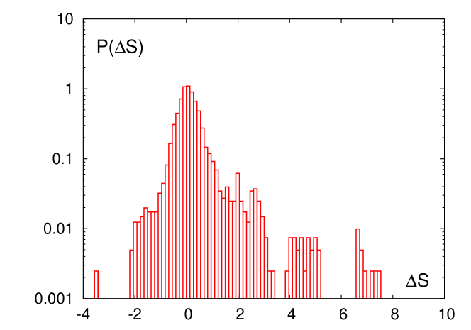
Figure 1: The histogram of the change in the action.

Let us denote the norm of a matrix $A$ by:

$$||A||=\sqrt{\sum_{i,j}|A_{ij}|^{2}}.$$

When we calculate the fermion force at each time step as an anti-Hermitian matrix defined on each link, we evaluate its norm and find the maximum value over the lattice: $||F||_{max}$. Also, at each time step we calculate the determinant of $V$ (Fat7 smeared) links and find the minimum value over the lattice: $|\det V|_{min}$. Time histories of these two quantities are shown in Fig. 2. Large values of the fermion force accompany small values of the determinant (or small eigenvalues) of Fat7 smeared links. Thus, when calculating smeared links by adding different paths one may by chance produce a matrix $V$ with an eigenvalue close to 0, which in turn leads to a large derivative $dW/dV$ (as in the U(1) example considered earlier) that results in a large fermion force. Our integration algorithm has a finite step size, so it is not able to integrate such “spikes” in the force smoothly, leading to instantaneous jumps in the action that we see as “outliers” in the action histogram Fig. 1.

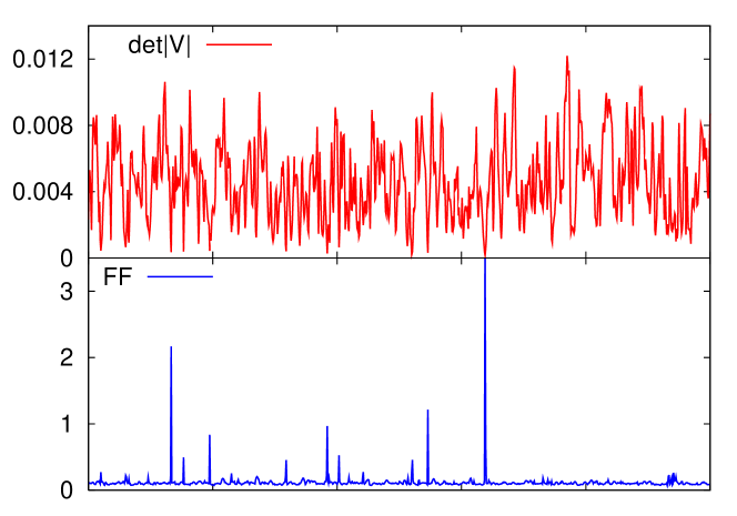
Figure 2: The time history of $|\det V|_{min}$ (top) and $||F||_{max}$ (bottom) for the $a=0.127$ fm ensemble during 5 time units ($=5\times 24=120$ time steps).

We investigated how this situation changes when we go to finer (smaller lattice spacing) ensembles. Since configurations become smoother, spikes in the force become less severe, as seen in Fig. 3.

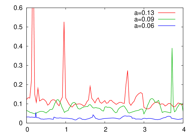
Figure 3: Fermion force $||F||_{max}$ for different ensembles versus time in time units (1 time unit corresponds to 24 steps for $a=0.127$, 32 steps for $a=0.093$ and 80 steps for $a=0.060$ ensemble).

4 Pion splittings on dynamical HISQ configurations

The effect of suppression of the taste-exchange interactions in HISQ was investigated in [1] by measuring the pion spectrum with valence HISQ on sea asqtad configurations. Here we report on similar measurements performed on dynamical HISQ configurations for the first two ensembles of Table 1.

It is convenient to define a dimensionless quantity which is almost independent of quark mass:

$$\Delta\equiv(M^{2}_{\pi}-M^{2}_{G})r_{1}^{2},$$ (6)

where $M_{G}$ corresponds to the Goldstone pion and $M_{\pi}$ refers to one of the other seven pion tastes in Tables 2 and 3. We calculate $\Delta$ for comparable asqtad and HISQ configurations, and then the ratio

$$R\equiv\frac{\Delta_{ASQ}}{\Delta_{HISQ}}$$ (7)

shows how much the splittings decrease when going from asqtad to HISQ. The values of $R$ for different pion tastes are shown in the last column of Tables 2 and 3. The statistical errors are rather large since for HISQ we have about an order of magnitude fewer configurations than for asqtad. The number of configurations used for measurements is indicated in parentheses in the headers of the second and third column. The overall trend is however clear and in agreement with Ref. [1]: about a factor of three improvement in taste symmetry for the HISQ action relative to asqtad.

Pion taste	$r_{1}\,M^{ASQ}_{\pi}$(658)	$r_{1}\,M^{HISQ}_{\pi}$(40)	$\Delta_{ASQ}$	$\Delta_{HISQ}$	$R$
$\gamma_{5}$	0.2244(02)	0.1889(07)
$\gamma_{0}\gamma_{5}$	0.2815(11)	0.2071(27)	0.029(1)	0.0072(11)	4.0(6)
$\gamma_{i}\gamma_{5}$	0.2822(05)	0.2058(10)	0.029(0)	0.0067(05)	4.4(3)
$\gamma_{i}\gamma_{j}$	0.3134(20)	0.2224(33)	0.048(1)	0.0138(15)	3.5(4)
$\gamma_{i}\gamma_{0}$	0.3126(11)	0.2188(19)	0.047(1)	0.0122(08)	3.9(3)
$\gamma_{i}$	0.3347(28)	0.2306(56)	0.062(2)	0.0175(26)	3.5(5)
$\gamma_{0}$	0.3373(15)	0.2311(22)	0.063(1)	0.0178(10)	3.6(2)
$\mathbb{I}$	0.359(5)	0.252(12)	0.079(4)	0.0280(61)	2.8(6)

Table 2: Pion spectrum on $a=0.127$ fm HISQ ensemble.

Pion taste	$r_{1}\,M^{ASQ}_{\pi}$(572)	$r_{1}\,M^{HISQ}_{\pi}$(50)	$\Delta_{ASQ}$	$\Delta_{HISQ}$	$R$
$\gamma_{5}$	0.2069(05)	0.1378(08)
$\gamma_{0}\gamma_{5}$	0.2177(10)	0.1420(08)	0.0046(5)	0.0012(4)	4(1)
$\gamma_{i}\gamma_{5}$	0.2187(07)	0.1428(08)	0.0050(4)	0.0014(3)	3.6(8)
$\gamma_{i}\gamma_{j}$	0.2256(11)	0.1467(21)	0.0081(5)	0.0025(7)	3.2(8)
$\gamma_{i}\gamma_{0}$	0.2259(07)	0.1475(11)	0.0082(4)	0.0028(4)	3.0(4)
$\gamma_{i}$	0.2311(15)	0.1485(16)	0.0106(7)	0.0031(5)	3.5(6)
$\gamma_{0}$	0.2318(10)	0.1509(11)	0.0109(5)	0.0038(4)	2.9(3)
$\mathbb{I}$	0.2398(25)	0.1522(27)	0.015(1)	0.0042(9)	3.5(8)

Table 3: Pion spectrum on $a=0.093$ fm HISQ ensemble.

5 Conclusions

In dynamical HISQ simulations with typical parameters, we found that smearing may produce a smeared link $V$ with a small eigenvalue that dominates the derivative of the reunitarized link $W$, $dW/dV$, and gives a large contribution to the fermion force. Such “spikes” in the force integrated with finite time steps give “jumps” in the action that decrease the acceptance rate of the RHMC algorithm. This problem was noted in Ref. [6] and is probably related to topological defects, “dislocations” that manifest themselves in plaquettes with low values lying on the tails of the plaquette distribution. We found that going to finer ensembles (smoother gauge configurations) reduces the number of spikes and partially cures the problem.

On configurations generated with the HISQ action for dynamical quarks we measured the staggered pion spectrum and found that pion splittings decrease by a factor of three or more, confirming the result of Ref. [1], where pioneering tests were done with valence HISQ fermions on configurations with asqtad sea quarks.

References

- [1] E. Follana, Q. Mason, C. Davies, K. Hornbostel, G.P. Lepage, J. Shigemitsu, H. Trottier and K. Wong, Phys. Rev. D 75, 054502 (2007) [arXiv:hep-lat/0610092v1].
- [2] S. Gottlieb, W. Liu, D. Toussaint, R. L. Renken and R. L. Sugar, Phys. Rev. D 35, 2531 (1987).
- [3] K. Y. Wong and R. M. Woloshyn, \posPoS(LAT2007) 047, 2007 [arXiv:0710.0737 [hep-lat]].
- [4] W. Kamleh, D. B. Leinweber and A. G. Williams, Phys. Rev. D 70, 014502 (2004) [arXiv:hep-lat/0403019].
- [5] C. Morningstar and M. J. Peardon, Phys. Rev. D 69, 054501 (2004) [arXiv:hep-lat/0311018].
- [6] A. Hasenfratz, R. Hoffmann and S. Schaefer, JHEP 0705, 029 (2007) [arXiv:hep-lat/0702028].
- [7] C. Aubin, C. Bernard, C. DeTar, Steven Gottlieb, E.B. Gregory, U.M. Heller, J.E. Hetrick, J. Osborn, R. Sugar, D. Toussaint, Phys. Rev. D 70, 094505 (2004) [arXiv:hep-lat/0402030].
- [8] A. Hart, G.M. von Hippel and R.R. Horgan, these proceedings.