Magnetic fields in axisymmetric neutron stars

Abstract

We derive general equations for axisymmetric Newtonian MHD and use these as the basis of a code for calculating equilibrium configurations of rotating magnetised neutron stars in a stationary state. We investigate the field configurations that result from our formalism, which include purely poloidal, purely toroidal and mixed fields. For the mixed-field formalism the toroidal component appears to be bounded at less than 7%. We calculate distortions induced both by magnetic fields and by rotation. From our non-linear work we are able to look at the realm of validity of perturbative work: we find for our results that perturbative-regime formulae for magnetic distortions agree to within 10% of the nonlinear results if the ellipticity is less than $0.15$ or the average field strength is less than $10^{17}$ G. We also consider how magnetised equilibrium structures vary for different polytropic indices.

1 Introduction

The physics of neutron stars classes them among the most extreme objects in the known Universe: their densities, rotation rates and magnetic fields are all among the highest known for any astrophysical object. Typical neutron star magnetic fields are up to $\sim 10^{12-13}$ G, whilst for magnetars this figure is $\sim 10^{15}$ G. Since magnetic fields induce a distortion in a star, a rotating magnetised neutron star could be a significant source of gravitational radiation. With the advent of second-generation gravitational wave detectors like Advanced LIGO, we may soon be in a position to observe neutron stars through their gravitational radiation signals — and hence have a new probe of the physics of these stars.

Understanding magnetic distortions requires an understanding of the neutron star’s interior field; NSs with relatively weak exterior fields could still have significant ellipticities if they have a much stronger field in their bulk. Here we model a NS as an infinitely conducting polytropic fluid and examine various kinds of magnetic field: purely poloidal, purely toroidal and mixed-field configurations. The numerical scheme we use is able to deal with extremely strong fields and fast rotation, so we are able to study the theoretical properties of very highly magnetised stars, as well as examining how well perturbative results hold away from the weak-field regime.

It has long been predicted that magnetic fields will distort a fluid star (Chandrasekhar & Fermi, 1953). It was found that this distortion only becomes appreciable if the magnetic energy $\mathcal{E}_{mag}$ of the star is comparable with its gravitational energy $W$; since neutron stars have tremendous self-gravity it follows that one would only expect very strong magnetic fields to generate any significant distortion. This suggests that one would expect magnetars to be the most distorted NSs and hence of most interest to gravitational wave astronomy (with the caveat that this early work is for an incompressible fluid and so is of limited relevance to NSs). For the results presented in this paper we will quantify this statement by scaling our code-generated results to real neutron star values.

A number of studies of magnetically deformed stars exist. These have included work focussed on poloidal, toroidal or mixed fields, and boundary conditions where the fields either vanish on the surface of the star or decay at infinity. Changing any of these can lead to very different results, so the uncertainty we have about the geometry of NS magnetic fields translates into an uncertainty about how distorted neutron stars are.

Analytic approaches have been restricted to weak fields and small deformations, as the nonlinear nature of stronger magnetic fields rapidly makes the problem intractable. Early work treated deformations of incompressible fluids (see, e.g., Ferraro (1954); Roberts (1955); Ostriker & Gunn (1969)), a simplifying assumption but not terribly physical for real stars. The first studies of compressible stars assumed very simplistic density distributions and magnetic fields confined within the star (Woltjer, 1960; Wentzel, 1961); later Goossens (1972) treated the problem of a poloidal field matched to an external dipole, extending the work of Ferraro (1954). More recently, work has focussed on the problem of magnetic deformations related specifically to neutron stars (Haskell et al., 2008), including a mixed-field case with vanishing exterior field.

In addition to analytic work, a number of studies have used numerical methods to calculate magnetic distortions. Monaghan (1965) and Roxburgh (1966) calculated field geometries and surface distortions for various polytropes, allowing for an exterior magnetic field. Their work was perturbative and so restricted to weak fields. More recently a second-order perturbation technique has been applied for the strong fields found in magnetars (Ioka, 2001). Other studies of highly magnetised stars have solved the fully non-linear problem, to allow for more highly deformed configurations than could be accurately determined using a perturbative approach. This was originally done for strong magnetic fields confined within the star (Ostriker & Hartwick, 1968), by extending an earlier self-consistent field method for rapidly-rotating stars (Ostriker & Mark, 1968). For purely poloidal fields an improved numerical method was devised which enabled the calculation of highly distorted equilibrium configurations (Miketinac, 1975); it was found that for very strong fields the maximum density of the star could move away from the centre to make the geometry of the density distribution toroidal. Solutions have also been found using a mixed-field formalism (Tomimura & Eriguchi, 2005). Finally, relativistic effects have been considered: fully relativistic solutions for purely poloidal fields (Bocquet et al., 1995) and purely toroidal fields (Kiuchi & Yoshida, 2008) and partially-relativistic solutions in the mixed-field case (Kiuchi & Kotake, 2008; Colaiuda et al., 2008). In the Discussion we shall return to the role of boundary conditions in the mixed-field case.

This paper is a study of the various stationary, axisymmetric equilibrium solutions for Newtonian fluid stars in perfect MHD. We show that the full equations of MHD reduce under these limits to two general cases: a mixed-field case (which includes purely poloidal fields as a special case) and purely toroidal fields. The mixed-field formalism dates back to Grad & Rubin (1958) and was recently used by Tomimura & Eriguchi (2005) to study mixed-field stars. We are not aware of any previous work using the other, purely toroidal, case for Newtonian MHD. In the mixed-field case the toroidal fields vanish outside the star, but the poloidal fields only decay at infinity; we consider this boundary condition more realistic than the condition of zero exterior fields used by much of the previous work discussed above. With our formalism, we investigate the resulting field configurations, including the relative strengths that toroidal and poloidal fields can have, and the maximum theoretical field strength a fluid star can have whilst remaining in an axisymmetric stationary equilibrium state. We also look at distortions induced by magnetic fields, including the effect of changing the polytropic index. We examine the validity of perturbative results for magnetic distortions in the strong-field regime. Finally, we rescale all our code results to canonical neutron star values and ensure we are always comparing magnetic and rotational effects in the same physical model star.

2 Axisymmetric formalism

2.1 Governing equations

We model a rotating magnetic neutron star by assuming that it is in a stationary state, axisymmetric with both the magnetic dipole axis and the spin axis aligned, and comprised of infinitely conducting material (the perfect MHD approximation). We work in electromagnetic units. The equations that describe this system are the Euler equation

$$-\frac{1}{\rho}\nabla P-\nabla\Phi_{g}+\nabla\Phi_{r}+\frac{\boldsymbol{\mathcal{L}}}{\rho}=0,$$ (1)

together with Poisson’s equation

$$\Delta\Phi_{g}=4\pi G\rho,$$ (2)

Ampère’s law

$$\nabla\times{\bf B}=4\pi{\bf j}$$ (3)

and the solenoidal constraint

$$\nabla\cdot{\bf B}=0.$$ (4)

We close the system of equations by assuming a barotropic equation of state:

$$P=P(\rho).$$ (5)

In the above equations $P,\rho,\Phi_{g},\Phi_{r},{\bf{j}},{\bf{B}},G$ and $\boldsymbol{\mathcal{L}}$ are the pressure, density, gravitational potential, centrifugal potential, current density, magnetic field, gravitational constant and Lorentz force ($\boldsymbol{\mathcal{L}}={\bf j\times B}$), respectively.

Although the formalism allows for different choices of the centrifugal potential $\Phi_{r}$ and equation of state $P=P(\rho)$, we will work with a rigidly rotating star:

$$\Phi_{r}=\frac{\Omega^{2}_{0}\varpi^{2}}{2},$$ (6)

where the angular velocity $\Omega_{0}$ is a constant and $\varpi$ the cylindrical polar radius; and a polytropic equation of state:

$$P=k\rho^{1+1/N},$$ (7)

where $k$ is some constant and $N$ the polytropic index.

The assumption of axisymmetry simplifies the equations considerably. Taking the curl of equation (1) leaves us with the requirement that

$$\nabla\times\left({\frac{\boldsymbol{\mathcal{L}}}{\rho}}\right)=0.$$ (8)

Additionally, the solenoidal nature of ${\bf B}$ allows us to write it in terms of some streamfunction $u$, defined through the relations

$$B_{\varpi}=-\frac{1}{\varpi}\frac{\partial{u}}{\partial{z}}\ ,\ B_{z}=\frac{1}{\varpi}\frac{\partial{u}}{\partial{\varpi}}.$$ (9)

One may also define a solenoidal ${\bf B}$-field by using the vector potential ${\bf A}$, where ${\bf B=\nabla\times A}$; we will use the $\phi$-component $A_{\phi}$ later. These two definitions are related by $u=\varpi A_{\phi}$. We also define a differential operator $\Delta_{*}$ by

$$\Delta_{*}\equiv\frac{\partial{{}^{2}}}{\partial{\varpi^{2}}}-\frac{1}{\varpi}\frac{\partial{}}{\partial{\varpi}}+\frac{\partial{{}^{2}}}{\partial{z^{2}}}.$$ (10)

Using the two conditions (8) and (9), one can show that Ampère’s law in axisymmetry may be rewritten as

$$4\pi{\bf j}=\frac{1}{\varpi}\nabla(\varpi B_{\phi})\times{\bf e}_{\phi}-\frac{1}{\varpi}\Delta_{*}\!u\ {\bf e}_{\phi}$$ (11)

— see section A.1 for a full derivation.

2.2 Mixed-field formalism

In axisymmetric perfect MHD with mixed poloidal and toroidal fields, the magnetic field and current are related through the Grad-Shafranov equation (see, e.g., Grad & Rubin (1958) or section A.2):

$$4\pi\rho\frac{d{M}}{d{u}}=-\frac{1}{\varpi^{2}}\left({\Delta_{*}\!u+f(u)\frac{d{f}}{d{u}}}\right),$$ (12)

where $f(u)\equiv\varpi B_{\phi}$ and $M(u)$ is defined through $\nabla M(u)\equiv\boldsymbol{\mathcal{L}}/\rho$. Combining the Grad-Shafranov equation with (11) yields

$${\bf j}=\frac{1}{4\pi}\frac{d{f}}{d{u}}{\bf B}+\rho\varpi\frac{d{M}}{d{u}}{\bf e}_{\phi}.$$ (13)

Finally we use the notation of Tomimura & Eriguchi (2005) and Chandrasekhar & Prendergast (1956), making the replacements $\alpha\equiv\frac{1}{4\pi}\frac{d{f}}{d{u}}$ and $\kappa\equiv\frac{d{M}}{d{u}}$, to arrive at our final expression relating the current and field:

$${\bf j}=\alpha(u){\bf B}+\varpi\rho\kappa(u){\bf e}_{\phi}$$ (14)

for a mixed poloidal and toroidal field in axisymmetry.

The two functions $\alpha(u)$ and $\kappa(u)$ govern different aspects of the magnetic field: firstly, since $\boldsymbol{\mathcal{L}}={\bf j}\times{\bf B}$ we have $\boldsymbol{\mathcal{L}}=\varpi\rho\kappa{\bf e}_{\phi}\times{\bf B}$ (from equation (14)) — i.e., the Lorentz force is dependent on $\kappa$, and so $\kappa$ governs the relative contributions of the magnetic and centrifugal forces to the overall distortion of the star. The role of $\alpha$ is less clear. From equation (14) we see that $\alpha=0$ gives a purely toroidal current and hence poloidal field, whilst increasing $\alpha$ increases the size of the mixed toroidal-poloidal term $\alpha{\bf{B}}$ (and so indirectly increases the toroidal component of the field). However, there is no limit in which the field is purely toroidal in this formalism. We can thus only expect $\alpha$ to have some indirect connection with the relative strengths of the poloidal and toroidal components of the magnetic field.

Following Tomimura & Eriguchi (2005), we choose the functional forms of $\alpha(u)$ and $\kappa(u)$ as:

$$\kappa(u)=\kappa_{0}=const.,$$ (15)

$$\alpha(u)=\begin{cases}a(u-u_{max})^{\zeta}&\textrm{if $u>u_{max}$}\\ 0&\textrm{if $u\leq u_{max}$,}\end{cases}$$ (16)

where $\alpha$ is chosen to ensure there is no exterior current, $\zeta$ is some constant and $u_{max}$ is the maximum surface value attained by the streamfunction $u$. Next we combine the definitions $\alpha\equiv\frac{d{f}}{d{u}}$ and $f(u)\equiv\varpi B_{\phi}$ to see that

$$\int^{u}\alpha(u^{\prime})\ du^{\prime}=\varpi B_{\phi}$$ (17)

— i.e., we must enforce the continuity of $\int\alpha(u)\ du$ to ensure the continuity of $B_{\phi}$. We therefore choose the lower limit of the integral of $\alpha$ so that

$$f(u)\equiv\int^{u}\alpha(u^{\prime})\ du^{\prime}=\begin{cases}\frac{a}{\zeta+1}(u-u_{max})^{\zeta+1}&\textrm{if $u>u_{max}$,}\\ 0&\textrm{if $u\leq u_{max}$.}\end{cases}$$ (18)

For our chosen functional forms of $\alpha(u)$ and $\kappa(u)$ we see that for a specific solution we need to choose three constants: $\zeta$, $a$ and $\kappa_{0}$. We will later drop the zero subscript, with the understanding that $\kappa$ always refers to a constant unless otherwise stated. Tomimura & Eriguchi (2005) set $\zeta=1$, but we have found that a smaller value of $\zeta$ allows for a slightly stronger toroidal-field component; accordingly, we set $\zeta=0.1$ throughout this paper, except in comparing our results with previous work (subsection 3.4).

For the purposes of numerics we seek integral equations; the integral form of (1) is

$$H=C-\Phi_{g}+\Phi_{r}+\int_{0}^{\varpi A_{\phi}}\kappa(u^{\prime})\ du^{\prime},$$ (19)

where $C$ is an integration constant and

$$H({\bf r})=\int_{0}^{P({\bf r})}\frac{dP^{\prime}}{\rho(P^{\prime})}$$ (20)

is the enthalpy.

The integral form of Poisson’s equation (2) is:

$$\Phi_{g}({\bf r})=-G\int\frac{\rho({\bf r}^{\prime})}{|{\bf r}-{\bf r}^{\prime}|}\ d{\bf r}^{\prime}.$$ (21)

Finally, using the current relation (14) an integral equation for the magnetic field may be found (see Tomimura & Eriguchi (2005) for details):

$$A_{\phi}({\bf r})\sin\phi=\int\frac{4\pi\frac{\alpha(\varpi^{\prime}A_{\phi}^{\prime})}{\varpi^{\prime}}\int_{0}^{\varpi^{\prime}A_{\phi}^{\prime}}\alpha(u)\ du+\kappa\rho\varpi^{\prime}}{|{\bf r}-{\bf r}^{\prime}|}\sin\phi^{\prime}\ d{\bf r}^{\prime}.$$ (22)

With the three equations (19), (21) and (22) it is possible to calculate stationary configurations of magnetised rotating stars (together with the specified constants $a$ and $\kappa$).

2.3 Toroidal-field formalism

For a purely toroidal field we have ${\bf{B}}=B_{\phi}{\bf{e}}_{\phi}$. In this case, the $\Delta_{*}\!u$ term disappears from equation (11) and the Lorentz force reduces to the form $\boldsymbol{\mathcal{L}}=B_{\phi}{\bf j}_{pol}\times{\bf e}_{\phi}$. Comparing these two expressions, one can show that $B_{\phi}$ is related to $\gamma\equiv\rho\varpi^{2}$ through some arbitrary function $h$ (which must vanish outside the star):

$$B_{\phi}=\frac{1}{\varpi}h(\gamma)$$ (23)

— see section A.4 for details. The magnetic potential for this case is:

$$M=-\frac{1}{4\pi}\int_{0}^{\rho\varpi^{2}}\frac{h}{\gamma}\frac{d{h}}{d{\gamma}}\ d\gamma,$$ (24)

where $\nabla M=\boldsymbol{\mathcal{L}}/\rho$ as before.

For simplicity we choose $h(\rho\varpi^{2})=\lambda\rho\varpi^{2}$ where $\lambda$ is a constant we specify for each code run. With this choice of $h$ we then have $B_{\phi}=\lambda\rho\varpi$ and $M=-\lambda^{2}\rho\varpi^{2}$, so that the first integral of the Euler equation becomes

$$H=C-\Phi+\textstyle{\frac{1}{2}}\Omega^{2}\varpi^{2}-\frac{1}{4\pi}\lambda^{2}\rho\varpi^{2}.$$ (25)

This equation, together with Poisson’s equation, is sufficient to find numerical solutions; the toroidal-field case is thus simpler than the mixed-field formalism, which also had an extra equation for the magnetic field.

2.4 Restrictions on the magnetic functions

In the appendix (outlined in the above sections) we show that for axisymmetric perfect MHD in a fluid, the equations reduce to a mixed-field case (with two magnetic functions $\alpha(u)$ and $\kappa(u)$) and a purely toroidal case (with a magnetic function $h(\gamma)$). Although the magnetic functions appear to be arbitrary, there are a number of restrictions on their functional forms, on either physical grounds or because they result in trivial solutions.

The functions $\alpha(u)$ and $h(\gamma)$ (where $u=\varpi A_{\phi}$ and $\gamma=\rho\varpi^{2}$ as before) govern the toroidal fields in the two cases, and so both must necessarily vanish outside the star to avoid having exterior currents. Since the streamfunction $u$ does not vanish at the star’s surface, we follow Tomimura & Eriguchi (2005) in defining $u_{max}$ to be the maximum surface value of $u$ and then choose $\alpha(u)$ to be a power of $(u-u_{max})$, which does vanish outside the star. There does not appear to be any other functional form for $\alpha$ which vanishes outside the star and is dependent only on $u$, so we conclude that (16) is the only acceptable choice for $\alpha(u)$. The functional form of $h$, similarly, appears restricted. To vanish outside the star $h(\gamma)$ cannot contain a constant piece, so let us consider a functional form of $h(\gamma)=\lambda\gamma^{\chi}$ where $\lambda$ and $\chi$ are constants. However, if $\chi<\frac{1}{2}$ then $B_{\phi}=\lambda\gamma^{\chi}\varpi^{-1}=\lambda\rho^{\chi}\varpi^{2\chi-1}$ will diverge at the origin, so we discard these choices. Additionally, we find that if $\chi>1$ is chosen, then the field iterates to zero in our numerical scheme, leading us to choose $h(\gamma)=\lambda\gamma$.

Finally, the function $\kappa(u)$ is theoretically allowed to depend on the streamfunction $u$, but if it is chosen as anything other than a constant then, as for $h(\gamma)$, we find that the configuration iterates to a zero-field solution. This may be a limitation of our numerical scheme rather than a physical restriction, but in either case our HSCF-scheme solutions are limited to those with $\kappa$ being equal to some constant.

We conclude from this that, in fact, the choices made for our functional forms are not specialised ones and (at least within our scheme) do not result in the exclusion of physically valid solutions. Rather, we believe that our results are quite generic to perfectly conducting polytropes in axisymmetry.

3 Numerics and calculating various quantities

3.1 Numerical scheme

Our code uses the Hachisu self-consistent field (HSCF) method (Hachisu (1986), extended to magnetised configurations by Tomimura & Eriguchi (2005)) to iteratively find a stationary solution to the hydromagnetic equilibrium equation (1). Specifically, one specifies a polytropic index $N$, magnetic functions $\alpha(u)$ and $\kappa(u)$ and the ratio of polar to equatorial radii $r_{p}/r_{eq}$, and the code determines the angular velocity, density distribution and other quantities consistent with the user’s input parameters.

The iterative steps for our extended (mixed-field) HSCF scheme are:

1. Make an initial guess of $\rho$=const.;
2. Find $\Phi_{g}$ from Poisson’s equation (21);
3. Guess $A_{\phi}$=const.;
4. Find an improved form of $A_{\phi}$ from equation (22) and the earlier guesses for $\rho$ and $A_{\phi}$ (this is the iterative step for $A_{\phi}$);
5. Find $\Omega_{0}^{2}$ and $C$ from the boundary condition that the enthalpy must vanish at the surface of the star; this requires the potentials $\Phi_{g}$ and $A_{\phi}$ found earlier and a user-specified axis ratio $r_{p}/r_{eq}$;
6. We now know all right-hand side terms in (19); use the equation to determine the enthalpy at all points in the star;
7. Find the new (improved) estimate for the density distribution using $\rho_{new}({\bf r})=\left({\frac{H({\bf r})}{H_{max}}}\right)^{N}$ where $N$ is the polytropic index and $H_{max}$ the maximum value of enthalpy attained in the star;
8. As the iterative step, return to step 1 but use $\rho=\rho_{new}$ instead of the earlier density distribution ($\rho$=const. for the first cycle). At step 3 in the new cycle, use the ‘new’ form of $A_{\phi}$ calculated in step 4 of the previous cycle.

This sequence of steps is repeated until the code has achieved satisfactory convergence in $H_{max}$, $\Omega^{2}_{0}$ and $C$. The toroidal-field scheme is similar to the one above except that the magnetic field is directly related to the density by $B_{\phi}=\lambda\rho\varpi$ for pure toroidal fields. For this reason there is no separate iteration in the magnetic field and steps 3 and 4 are no longer needed. The magnetic field only enters in step 6, where the enthalpy $H$ is found from the pure-toroidal equation (25) instead of the mixed-field version (19).

3.2 Magnetic energy and field strength

We will wish to calculate the magnetic energy $\mathcal{E}_{mag}$ of the star in the code, to compare different configurations and also to calculate a virial test (see section 3.3 and figure 1). The familiar definition of $\mathcal{E}_{mag}$ is

$$\mathcal{E}_{mag}=\int\limits_{\textrm{all space}}\frac{B^{2}}{8\pi}\ \ d{\bf r},$$ (26)

but this is not suited to numerical evaluation, since the integrand only decays at infinite distance; our numerical integration is over a finite radius and so this definition would introduce truncation error. However a physically equivalent definition for $\mathcal{E}_{mag}$, more useful here, is

$$\mathcal{E}_{mag}=\int\limits_{\textrm{all space}}{\bf r}\cdot\boldsymbol{\mathcal{L}}\ \ d{\bf r}$$ (27)

— since $\boldsymbol{\mathcal{L}}$ has compact support (through its $\rho$ dependence) the above integrand will vanish outside the star.

For a measure of the magnetic field strength of the star, we define a volume-averaged magnetic field $\bar{B}$ through

$$\bar{B}^{2}\equiv\frac{1}{V}\!\!\int\limits_{\textrm{all space}}\!\!B^{2}\ d{\bf r}=\frac{8\pi\mathcal{E}_{mag}}{V}.$$ (28)

3.3 Virial test

We may use the scalar virial theorem (see, e.g., Shapiro & Teukolsky (1983)) as a test of convergence for the code. For a rotating magnetised self-gravitating fluid the virial theorem states that

$$\frac{1}{2}\frac{d{{}^{2}I}}{d{t^{2}}}=2T+\mathcal{E}_{mag}+\frac{3U}{N}+W$$ (29)

where $I$ is the moment of inertia about the rotation axis and $T,\mathcal{E}_{mag},U$ and $W$ are the kinetic, magnetic, internal and gravitational energies, respectively. For our stationary star $I$ has no time variation so the first term is zero. Given this, we expect the various energies for our star to satisfy

$$2T+\mathcal{E}_{mag}+\frac{3U}{N}+W=0.$$ (30)

Calculating the quantity on the left-hand side of the above equation tells us the absolute deviation from zero, but we need to know the relative error. A value of $2T+\mathcal{E}_{mag}+3U/N+W=10^{-5}$ would appear to indicate acceptable accuracy, but if the individual energies are of order $10^{-4}$ then the relative error is unacceptable: around 10%. For this reason we normalise by dividing through by $W$ and define our virial test result $VC$ as

$$VC\equiv\frac{|2T+\mathcal{E}_{mag}+3U/N+W|}{|W|}$$ (31)

— the smaller the value of $VC$, the greater the code’s accuracy. We use $VC$ in our convergence testing, figure 1. In the figure we see that as grid resolution is increased the virial test result decreases; in particular, since the gradient of each plot is approximately $-1$ we conclude that the code is first-order convergent.

\psfrag{a}{(a)}\psfrag{b}{(b)}\psfrag{c}{(c)}\psfrag{MP}{$MP$}\psfrag{VC}{$VC$}\includegraphics[width=433.62pt]{convs.eps}

Figure 1: Convergence tests for: (a) a purely poloidal field, no rotation, axis ratio of 0.2; (b) mixed field with 2% toroidal field, no rotation, axis ratio of 0.2; (c) purely toroidal field, no rotation, axis ratio of 1.05. Here $VC$ is the virial test result and $MP$ the number of mesh points. Since $VC$ decreases as $MP$ increases, we see that the code is convergent.

3.4 Comparison with previous work

As a confirmation of our results, we compare with table 4 from Tomimura & Eriguchi (2005). Their results are nondimensionalised by dividing by appropriate powers of $\rho_{max}$, $r_{eq}$ and $4\pi G$ and these dimensionless quantities are denoted by a hat; for example

$$\hat{\Omega}^{2}=\frac{\Omega^{2}}{4\pi G\rho_{max}}.$$ (32)

For comparison with their results we must also use $\zeta=1$ instead of $\zeta=0.1$ as the exponent in the functional form of $\alpha$ from (16). Taking this into account we find that for a $N=1.5$ polytrope, with $\hat{\kappa}=0.4$ and $\hat{a}=200$, we have the sequence of configurations given in table 1.

Table 1: Dimensionless quantities for a sequence of stars with $N=1.5,\hat{\kappa}=0.4,\hat{a}=200$ and $\zeta=1$.

$r_{p}/r_{eq}$	$\mathcal{E}_{mag}/|W|$	$U/|W|$	$T/|W|$	$|\hat{W}|$	$\hat{\Omega}^{2}$	$\hat{M}$	$VC$
0.588	0.144	0.284	1.21e-03	4.81e-02	5.14e-04	0.831	2.97e-05
0.55	0.151	0.276	1.11e-02	4.59e-02	4.53e-03	0.811	3.10e-05
0.50	0.165	0.264	2.11e-02	4.32e-02	8.01e-03	0.787	3.33e-05
0.45	0.189	0.255	2.27e-02	4.01e-02	7.72e-03	0.763	3.63e-05
0.40	0.222	0.252	1.19e-02	3.58e-02	3.45e-03	0.729	4.02e-05
0.371	0.242	0.252	1.10e-03	3.31e-02	2.89e-04	0.705	4.32e-05

Our highest and lowest axis ratios ($0.588$ and $0.371$) differ slightly from those of Tomimura & Eriguchi (2005) (who have $0.589$ and $0.372$), so we cannot make a direct comparison for these values. However for the other four axis ratios our values agree to within $\sim 8\%$ for $\hat{\Omega}^{2}$ and $T/|W|$, and to within $\sim 1\%$ in all other quantities. We also show our results for the virial test, showing that all our results have relative errors of $\sim 10^{-5}$.

3.5 Toroidal and poloidal energies for the mixed case

The code variables $\kappa$ and $\alpha$ are related to the ratio of toroidal to poloidal field strength, but in a very nontrivial manner. To get a more intuitive, physical, measure of their respective strengths we would like to know the part of the magnetic energy contained in the poloidal and toroidal fields, $\mathcal{E}_{pol}$ and $\mathcal{E}_{tor}$, respectively.

Since the total magnetic energy is given by

$$\mathcal{E}_{mag}=\frac{1}{8\pi}\int{\bf{B\cdot B}}\ d{\bf r}=\frac{1}{8\pi}\int\left({B_{\varpi}^{2}+B_{\phi}^{2}+B_{z}^{2}}\right)\ d{\bf r},$$ (33)

we define the poloidal energy by

$$\mathcal{E}_{pol}=\frac{1}{8\pi}\int\left({B_{\varpi}^{2}+B_{z}^{2}}\right)\ d{\bf r}=\frac{1}{2}\int_{0}^{1}\int_{0}^{\infty}\left({B_{\varpi}^{2}+B_{z}^{2}}\right)\ drd\mu$$ (34)

and the toroidal energy by

$$\mathcal{E}_{tor}=\frac{1}{8\pi}\int B_{\phi}^{2}\ d{\bf r}=\frac{1}{2}\int_{0}^{1}\int_{0}^{\infty}B_{\phi}^{2}\ drd\mu$$ (35)

where the integration here is over spherical polars $r$ and $\mu\equiv\cos\theta$. Note that since $B_{\phi}=0$ outside the star, the toroidal-energy integral only needs to be evaluated over the stellar interior. For our mixed-field configurations we use $\mathcal{E}_{tor}/\mathcal{E}_{mag}$ as a measure of the proportion of toroidal field.

3.6 Ellipticity

For the code we specify the axis ratio $r_{p}/r_{eq}$, which measures the distortion of the star’s surface. For a measure of the distortion of the whole mass distribution of the star we define an ellipticity $\epsilon$ through the (unreduced) quadrupole moments at the equator $I_{eq}$ and the poles $I_{p}$:

$$\epsilon\equiv\frac{I_{eq}-I_{p}}{I_{eq}}.$$ (36)

3.7 Constructing physical sequences of stars

To make a meaningful study of a group of different equilibrium configurations requires ensuring that we are always comparing the effects of magnetic fields and rotation in the same physical star: we do this by ensuring that we work with sequences of constant (physical) mass and the same equation of state — i.e. both the same polytropic index $N$ and polytropic constant $k$. We note that other intuitively sensible choices, for example just fixing the equatorial radius or central density, would mean comparing stars of either different mass or different equation of state. This would make quantifying the effects of magnetic fields and rotation more difficult.

We fix our neutron star mass to the generic value of $M=1.4M_{\odot}=2.8\times 10^{33}$ g. For the equation of state we work with $N=1$ polytropes and fix $k$ by requiring that the radius $R$ of the equivalent unmagnetised nonrotating (and hence spherical) star is 10 km. We will term this star the ‘background’ star, with the understanding that this refers to a configuration without magnetic fields or rotation, rather than having any perturbation theory connotations. Using the ($N=1$) polytropic relation $R=\sqrt{\pi k/2G}$ we see that this gives a polytropic constant of $4.25\times 10^{4}$ g^-1cm⁵s^-2. For the rest of this paper, when we quote physical parameters they will be for our ‘canonical neutron star’ with $M=1.4M_{\odot}$ and $k=4.25\times 10^{4}$ g^-1cm⁵s^-2.

For the plots where we have used different polytropic indices the redimensionalising is less straightforward, as the relation between spherical radius $R$ and $k$ also includes powers of the ‘background’ central density $\rho_{c}$ (see Chandrasekhar (1939) for the required polytropic relations). For these cases we again fix the mass at $1.4M_{\odot}$ and fix the background central density at $\rho_{c}=2.19\times 10^{15}$ g cm^-3 — the same value as for the background $N=1$ star discussed above. This then fixes $R$ and $k$.

4 Magnetic field configurations

\psfrag{a}{(a)}\psfrag{b}{(b)}\psfrag{c}{(c)}\psfrag{d}{(d)}\includegraphics[width=433.62pt]{Bcontour.eps}

Figure 2: Contours of magnetic field strength. Plots (a), (b), (c) are (respectively) the poloidal, toroidal and total magnetic field strength for our canonical NS with a mixed-field configuration consisting of 3.0% toroidal field. Plot (d) is for magnetic field strength in a purely toroidal-field star. Note how the toroidal field in this case is much more extensive than in the mixed-field plot (b). In plots (a) and (c) the maximum field strength is $5.5\times 10^{17}$ G (at the origin) and the contour separation is $5.5\times 10^{16}$ G. For plots (b) and (d) the maximum field occurs in the centre of the torus bounding the toroidal field; the maximum values are $2.6\times 10^{17}$ G and $2.8\times 10^{17}$ G, with contour separations of $2.9\times 10^{16}$ G for both plots. The bold red line in each plot represents the star’s surface; the values on the axes show the nondimensional radius $r/r_{eq}$ (where $r$ is the physical radius).

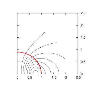
Figure 3: Contours of the streamfunction $u$ for a purely poloidal-field star; these contours are parallel to magnetic field lines and so represent the direction of the field. The surface of the star is the bold red line. Field lines for the toroidal component of a mixed-field star, or for purely toroidal stars, would go into the page and hence are not plotted here.

\psfrag{N}{$N$}\psfrag{B_ratio}{$\displaystyle\frac{B_{p}}{\bar{B}}$}\includegraphics[width=173.44534pt]{N-Bratio.eps}

Figure 4: Left: the ratio of polar field to volume-averaged field, $B_{p}/\bar{B}$, as a function of the polytropic index $N$. The plot is for purely poloidal fields in non-rotating stars, all with an axis ratio of $0.996$. Note that if the field was purely toroidal then this ratio would be zero, regardless of $N$.

With the formalism described above, we are able to examine the field configurations generated in axisymmetric perfectly conducting polytropes. Since neutron star matter is thought to have high conductivity and be roughly approximated by an $N=1$ polytrope, the field structures shown here should have some similarity to those in real neutron stars — although the field strengths here are considerably higher than those that have been observed so far. The plots in this section show contours of the magnetic field strength given by $|{\bf B}|=\sqrt{{\bf B}\cdot{\bf B}}$, and of the poloidal and toroidal components, $|{\bf B}_{pol}|=\sqrt{B_{\varpi}^{2}+B_{z}^{2}}$ and $|{\bf B}_{tor}|=|B_{\phi}|$. All of the magnetic-field results presented here (and discussed in this section) are for non-rotating $N=1$ polytropes, unless otherwise stated. In addition, we have concentrated on mixed-field configurations here, since there are strong indications from both theory (Markey & Tayler, 1973; Tayler, 1973; Wright, 1973) and simulations (Braithwaite & Nordlund, 2006) that both purely poloidal and purely toroidal fields are generically unstable.

In figure 2 we plot the poloidal (plot (a)) and toroidal (plot (b)) components of a mixed-field star and the total field of the configuration (plot (c)). We also plot the field structure of a star generated from our purely toroidal-field formalism for comparison (plot (d)). We see that the poloidal field pervades most of the interior of the mixed-field star, as well as extending outside it. This component of the field is highest in the centre and only goes to zero in a small region at the edge of the star (seen as the pair of semicircular contours on the equator at $x\sim 0.8$); Markey & Tayler (1973) call this zero-field point the ‘magnetic axis’. By contrast the toroidal field is wholly contained within this small region where the poloidal field vanishes; this region is dictated by the functional form of $\alpha(u)$ that we use. All configurations shown in this section are non-rotating, but rotation does not greatly affect the nature of the magnetic field.

Comparing plots (b) and (d) in figure 2 we see that, although the maximum field strengths and contours are of similar magnitude in the two cases, the field in the pure-toroidal case extends over a far larger region of the star than the toroidal part of the mixed-field configuration.

Figure 2 shows the magnitude of the magnetic field at a particular point; in figure 3 we show the direction of a typical poloidal field by plotting contours of the streamfunction $u$. These contours are parallel to magnetic field lines, from section A.2 of the appendix. Since a purely toroidal field has direction vector ${\bf e}_{\phi}$, the field lines would go into the page in the $x-z$ plane we employ here (they would form concentric circles in the $x-y$ plane). Mixed-field lines lie in neither plane so we have not shown them here.

Lastly in this section, figure 4 shows the dependence of the ratio $B_{p}/\bar{B}$ on the polytropic index $N$; we find that there is an approximately linear relationship between the two, and for all polytropic indices $B_{p}/\bar{B}$ is of the same order of magnitude. For $N=1$, $B_{p}/\bar{B}\approx 0.5$, suggesting that neutron stars (approximated as $N=1$ polytropes) with purely poloidal fields are likely to have a $\bar{B}$ around double the polar field $B_{p}$.

4.1 The relationship between $a$ and $\mathcal{E}_{tor}/\mathcal{E}_{mag}$

Table 2: Comparing parameters related to the influence of the toroidal component in a mixed-field star with axis ratio $0.9$.

$a$	$\mathcal{E}_{tor}/\mathcal{E}_{mag}$	$\mathcal{E}_{mag}/|W|$	$\epsilon$	$B_{p}/\bar{B}$
0	0.00	2.43e-02	0.216	0.580
10	9.87e-03	2.55e-02	0.216	0.554
20	3.02e-02	2.82e-02	0.213	0.504
30	3.96e-02	2.93e-02	0.204	0.484
40	4.05e-02	2.92e-02	0.196	0.488
50	3.86e-02	2.88e-02	0.191	0.495

As mentioned earlier, we can increase the proportion of toroidal field in the mixed-field configurations only indirectly, by varying the code parameter $a$ from equation (16). In table 2 we show the effect of changing this parameter, for a non-rotating star with axis ratio $r_{p}/r_{eq}=0.9$. One would expect that increasing $a$ would increase the toroidal portion of the field, which in turn would lead to a decrease in oblateness (since toroidal fields induce prolate distortions); one would also expect a reduction in the ratio $B_{p}/\bar{B}$ (since more of the field is toroidal and hence does not extend outside the star). Looking at the table, we see all of these effects do occur as the value of $a$ is increased, up until the $a=40$ configuration. At this point the larger value of $a$ is no longer reflected in stronger toroidal-field effects. In all cases changing $a$ does not strongly affect the value of $\mathcal{E}_{mag}/|W|$, confirming our expectation that it is the variation in the toroidal component which affects ellipticity and $B_{p}/\bar{B}$, rather than simply a reduction in $\mathcal{E}_{mag}/|W|$. Finally, we note that even for the highest values of $a$, the relative contribution of the toroidal portion of the field is very small — only 4% of the total here. We shall see later that this is a generic feature of our formalism together with our boundary condition, where poloidal fields extend outside the star but toroidal ones vanish at the surface.

5 Magnetic and rotational distortions

\psfrag{(a)}{(a)}\psfrag{(b)}{(b)}\psfrag{(c)}{(c)}\psfrag{(d)}{(d)}\includegraphics[width=303.53267pt]{densmag_paper.eps}

Figure 5: Nonrotating $N=1$ polytropes distorted by the effect of a poloidal magnetic field, with axis ratios of $0.7,0.5,0.2,0.0$ (from (a) to (d)). For increasing distortion the maximum density moves away from the centre and the density distribution becomes toroidal (in the sense that the maximum density moves away from the centre of the star). As before, the numbers on the axes are dimensionless, but for our canonical NS $r_{eq}=11.4,12.9,16.2,17.0$ km for plots (a)-(d).

\psfrag{(a)}{(a)}\psfrag{(b)}{(b)}\psfrag{(c)}{(c)}\psfrag{(d)}{(d)}\includegraphics[width=303.53267pt]{r06_dens.eps}

Figure 6: Density contours in an $N=1$ polytropic star with axis ratio of 0.6, with different sources of distortion. Plots (a), (b) and (c) are nonrotating configurations with, respectively: purely poloidal field, mixed-field with 3.4% toroidal field, mixed-field with 5.5% toroidal field. Plot (d) is for a purely rotationally-distorted star with no magnetic field. All stars have the canonical mass of $1.4M_{\odot}$, with equatorial radii of $12.1,12.5,13.2,14.4$ km for stars (a)-(d), respectively. We note that whilst a purely poloidal field tends to push the maximum density away from the centre, both toroidal field components and rotation have the effect of increasing the equatorial radius and making the star more diffuse.

Having looked at field configurations, we now turn to the distortions these fields produce in the star’s mass distribution. For purely poloidal fields we confirm previous work that these fields induce an oblate distortion; the surface shapes of such stars are thus similar to those of rotationally distorted stars. However, the interior density distributions are very different: centrifugal forces tend to leave a smaller high-density central region, whilst the Lorentz force acts to pull the point of maximum density away from the centre into a maximum-density ring. In the extreme limit where the ratio $r_{p}/r_{eq}\to 0$, the star actually becomes a torus (figure 5). For mixed fields, the effect of increasing the toroidal component is similar to the effect of adding rotation: it tends to push the maximum density region back to the centre — see figure 6. Note that both the mixed-field stars shown are oblate though, due to the dominance of the poloidal component; stronger toroidal fields tend to make stars prolate, but our formalism and boundary condition seem to generate mixed fields with weak toroidal components only (the 5.5%-toroidal field of figure 6 plot (c) is relatively strongly toroidal, within this context).

For weak fields and small distortions, perturbation theory results suggest that the ellipticity of a star should depend linearly on $B^{2}$. With our non-linear code we are able to check this, and see how well the perturbative result holds as field strengths are increased; this is plotted for both poloidal and toroidal fields in figure 7. The results depart slowly from the linear regime to begin with, but in the poloidal-field case the field strength required reaches a peak and then decreases again, for increased ellipticity. This peak seems to correspond to roughly the point at which the maximum density is pulled out into a ring, making the star’s density distribution toroidally-shaped. We speculate that for very low axis ratios (i.e. very strong fields), this toroidally-shaped density is a more stable, lower-energy state than one where the maximum density remains at the centre.

Purely toroidal fields give prolate density distributions, although we find that the surface shape remains virtually spherical even for large ellipticities (i.e. strong fields). Because rotation gives rise to oblateness in stars, it opposes the effect of a toroidal field in a star, and the two effects can balance to give a rotating magnetised star with zero overall ellipticity. Note that in this case the stars will have oblate surface shapes but a spherical density distribution — see figure 8.

Next we look at the effect of magnetic fields on the Keplerian velocity $\Omega_{K}$ — see figure 9. We find that whilst increasing the field strength causes a slight decrease in the velocity needed to cause mass shedding, this effect only becomes noticeable for very strong fields. It seems, therefore, that magnetic fields are unlikely to affect the stability of a star in this manner.

We have generally presented results for an $N=1$ polytrope, as this is regarded as a reasonable approximation to a neutron star. For our final two figures, however, we briefly investigate the effect of varying the polytropic index $N$, whilst maintaining a mass of $1.4M_{\odot}$ and central density of $2.19\times 10^{15}$ g cm^-3 in the corresponding unmagnetised ‘background’ polytropic star. In figure 10, we plot four stars with the same surface distortion $r_{p}/r_{eq}=0.5$ but different $N$. We see that when $N$ is low the density contours are all close to the edge of the star, with a large (slightly off-centre) high-density region; in the limiting case $N=0$ the star is an incompressible, uniform density configuration, so all contour lines coincide with the star’s surface. For higher values of $N$ the high-density region becomes smaller and the low-density outer region becomes larger. We note that the $N=2$ polytrope shown cannot be a neutron star model, however, as its maximum density of $1.79\times 10^{14}$ g cm^-3 is lower than the density of heavy nuclei, $\rho_{0}=2.4\times 10^{14}$ g cm^-3.

Finally, in figure 11, we look at non-rotating stars magnetised by a purely poloidal field, with an axis ratio of $0.95$. We plot the dependence of the field strength on polytropic index $N$, finding that as $N$ is increased a weaker field is required to support the same surface distortion.

\psfrag{distortion}{\emph{distortion}}\psfrag{eps}{$\epsilon$}\psfrag{1-r_B}{$1-\frac{r_{p}}{r_{eq}}$}\psfrag{Bsq}{$\displaystyle{\left({\frac{\bar{B}}{10^{17}\textrm{ G}}}\right)^{2}}$}\includegraphics[width=433.62pt]{B2-poldist.eps}

\psfrag{eps}{$\displaystyle\epsilon$}\psfrag{epsi}{$-\displaystyle\epsilon$}\psfrag{B}{$\displaystyle{\left({\frac{\bar{B}}{10^{17}\textrm{ G}}}\right)^{2}}$}\includegraphics[width=433.62pt]{B2-tordist.eps}

Figure 7: Left: a graph showing how (poloidal) magnetic distortions vary with the field strength. $1-r_{p}/r_{eq}$ is the surface distortion, whilst $\epsilon$ represents the distortion of the density distribution, as defined in equation (36). Note that the required field strength peaks for $1-r_{p}/r_{eq}\sim 0.6$ or $\epsilon\sim 0.8$ and then drops slightly for more extreme distortions. For small distortions we see that there is a roughly quadratic dependence on the field strength. Right: toroidal-field distortions versus $B^{2}$. In this case we only use $\epsilon$ to gauge the level of distortion, as the surface shapes remain nearly spherical.

Figure 8: Two stars with toroidal magnetic fields. The left-hand configuration is a non-rotating star (and hence has a prolate density distribution), whilst the right-hand one is the same physical star but with rotation added, with an oblate surface shape but an overall ellipticity of zero. The average field strength in both cases is $\bar{B}=2.4\times 10^{17}$ G.

\psfrag{B}{$\displaystyle{\frac{\bar{B}}{10^{17}\textrm{ G}}}$}\psfrag{Om_K}{$\displaystyle{\frac{\Omega_{K}}{2\pi}}$ / Hz}\includegraphics[width=173.44534pt]{BvsOm_K.eps}

Figure 9: The dependence of Keplerian velocity $\Omega_{K}$ on magnetic field strength $\bar{B}$, for stars with purely poloidal fields. Note that an appreciable decrease in $\Omega_{K}$ only occurs for very strong fields.

\psfrag{(a)}{(a)}\psfrag{(b)}{(b)}\psfrag{(c)}{(c)}\psfrag{(d)}{(d)}\includegraphics[width=303.53267pt]{varyN.eps}

Figure 10: Non-rotating configurations, all with a purely poloidal field and an axis ratio of $r_{p}/r_{eq}=0.5$. Plots (a) to (d) are for $N=0.5,1,1.5,2$ polytropes, respectively; the corresponding field strengths are $\bar{B}=7.62,4.31,2.98,1.13\ \times 10^{17}$ G, the maximum densities are $1.67,1.14,0.623,0.179\times 10^{15}$ g cm^-3 and the equatorial radii are $r_{eq}=10.2,12.9,17.6,29.6$ km, respectively.

\psfrag{N}{$N$}\psfrag{Bav}{$\displaystyle{\frac{\bar{B}}{10^{17}\textrm{ G}}}$}\includegraphics[width=173.44534pt]{BvsNfig.eps}

Figure 11: Right: the poloidal field strength $\bar{B}$ required to induce a surface distortion of $r_{p}/r_{eq}=0.95$, plotted for various polytropic indices. We see that the required field is weaker for higher-$N$ polytropes.

6 Discussion

To understand how strong magnetic distortions may be in highly magnetised objects like magnetars, realistic models are needed to study the field structure of these stars. The formalism we use in this work comes directly from the assumptions of axisymmetry and perfect conductivity, together with a boundary condition that the poloidal part of the field should decay at infinity rather than vanishing at the star’s surface; we anticipate that these conditions provide a reasonable model of a neutron star’s field.

The general formalism of axisymmetric MHD reduces to a mixed-field case and a purely toroidal-field case, with two (mathematically) arbitrary functions in the former case ($\kappa(u)$ and $\alpha(u)$) and one in the latter ($h(\gamma)$). Despite the apparent freedom in choosing these functions, we found that on physical grounds only one functional form was satisfactory for each one; see section 2.4. We conclude that the equations we have numerically solved in this work are in fact quite general and that we have not excluded physically valid branches of solutions with our choices.

Perturbative calculations in the weak-field regime have found that $\epsilon$ depends linearly on $\bar{B}^{2}$. With the use of our nonlinear code we are able to investigate how well this approximation holds for larger fields and ellipticities. We can see graphically that the first few points from both plots in figure 7 lie in fairly straight lines and hence we deduce the relations

$$\epsilon_{pol}\sim 5\times 10^{-4}\left({\frac{\bar{B}}{10^{16}\textrm{ G}}}\right)^{2}\sim 2\times 10^{-3}\left({\frac{B_{p}}{10^{16}\textrm{ G}}}\right)^{2}$$ (37)

for the purely poloidal case (the above relation also uses $B_{p}/\bar{B}\sim 0.5$ from figure 4), and

$$\epsilon_{tor}\sim-3\times 10^{-4}\left({\frac{\bar{B}}{10^{16}\textrm{ G}}}\right)^{2}$$ (38)

for the purely toroidal case; where in both cases we have used a star of mass $1.4M_{\odot}$ whose radius would be 10 km if unmagnetised. By comparing these extrapolated linear-regime formulae with our non-linear code results, we can explore how well perturbative results are likely to hold in a strong-field regime. We find that the linear regime given by (37) and (38) differs by less than 10% of the actual non-linear code result (shown in figure 7) provided that $\bar{B}\lesssim 1.5\times 10^{17}$ G, or equivalently $\epsilon\lesssim 0.15$. Alternatively, if we allow the linear relation to differ by up to 30% from the nonlinear result, we may use the linear relation as an ‘acceptable’ approximation for $\bar{B}\lesssim 3\times 10^{17}$ G or $\epsilon\lesssim 0.35$ (i.e. it holds for the entire range of ellipticities we can plot in the toroidal-field case).

This suggests that for all known neutron star field strengths, $\epsilon$ is likely to be linearly dependent on $\bar{B}^{2}$, to a good approximation. Hence perturbation theory could provide accurate predictions of NS distortions, provided the neutron star model used is also a close approximation to real NS physics.

We are also able to compare our linear-regime formulae with the analytic work of Haskell et al. (2008), who also treated pure poloidal fields extending outside the star and pure toroidal fields vanishing at the stellar surface (as for our work). For the same mass, radius and polytropic index their formulae give:

$$\epsilon_{pol}\sim 10^{-2}\left({\frac{B_{s}}{10^{16}\textrm{ G}}}\right)^{2}\ \textrm{ and }\ \epsilon_{tor}\sim-2\times 10^{-4}\left({\frac{\bar{B}}{10^{16}\textrm{ G}}}\right)^{2}$$ (39)

where $B_{s}$ is the surface magnetic field strength, which was assumed constant for the calculation of Haskell et al. (2008); we do not have a constant surface field so have compared with their work using the value of $|{\bf{B}}|$ at the pole instead. Since their field geometries are clearly not identical to ours, and since we had to extrapolate to obtain our formulae, we would not expect precise agreement. Nonetheless, we feel that the similarities show that our work makes sensible contact with perturbative calculations.

From figure 7, beginning at an unmagnetised spherical star, we find that in both the poloidal and toroidal cases the magnetic field strength required increases for larger distortions, initially; as would be expected from perturbative work. However, in the purely poloidal case the field strength then peaks at $\epsilon\sim 0.8$, dropping slightly as $\epsilon$ is increased further. Around the same point the density distribution becomes toroidal in nature — that is, the point of maximum density moves away from the centre and a high-density torus forms; this leads us to speculate that at $\epsilon\sim 0.8$ it becomes energetically favourable for the density to change from a spheroidal profile (as seen in the weaker-field stars, e.g. figure 5, plot (a)) to a toroidal one (e.g. figure 5, plot (d)). It is clear that if the magnetic field in a star is increased beyond the peak value of $\sim 5\times 10^{17}$ G shown in the left-hand plot of figure 7 then one of our initial assumptions must be violated. Since we cannot investigate the possibilities with our current code, we conclude that a hypothetical star with a field of $\bar{B}>6\times 10^{17}$ may either have no equilibrium solution (in which case it may lose magnetic energy until it is in equilibrium), or that there may be a new triaxial branch of super-magnetised solutions bifurcating from the biaxial curve at $\epsilon\sim 0.8$.

We do not find a similar peaking of the field strength in the purely toroidal case, however. In this case the largest ellipticities we are able to calculate are around $\epsilon\sim 0.35$. Whilst this particular value may represent a limitation of our numerical scheme, we suggest that a limited range of ellipticities is a consequence of the formalism for toroidal fields in axisymmetry, where ${\bf B}$ is directly linked to the density $\rho$; in the mixed-field case we have a separate equation to iteratively solve for the magnetic field. Thus restrictions on the field geometry may restrict the size of permissible ellipticities.

Of course, whilst the ‘peak field strength’ we discuss here is a theoretical upper bound on NS fields, there are probably other physical effects that place a lower bound than $\sim 5\times 10^{17}$ G on the maximum field. Certainly, if magnetar surface fields are $\sim 10^{15}$ G one would not expect their volume-averaged fields to exceed $\sim 10^{16}$ G.

We have argued that the equations we solve in this paper lead to quite general solutions for axisymmetric stars. However, we find that although it is possible to find solutions with purely poloidal or purely toroidal fields, the range of mixed-field solutions is very limited. Using $\mathcal{E}_{tor}/\mathcal{E}_{mag}$ as a gauge of the strength of the toroidal component in a mixed-field star, we find that for all our stars $0\leq\mathcal{E}_{tor}/\mathcal{E}_{mag}<0.07$. The other extreme is of course $\mathcal{E}_{tor}/\mathcal{E}_{mag}=1$ for purely toroidal fields. This means that although the toroidal component does have some influence in a mixed-field star (see table at the end of section 4), it is dominated by the effect of the poloidal field. In particular all our mixed-field stars have oblate density distributions.

Our mixed-field stars have the boundary condition that the toroidal component vanishes at the surface, whilst the poloidal piece only decays at infinity. By contrast, Haskell et al. (2008) considered the problem of mixed-field stars where the total field vanished at the surface. This results in an eigenvalue problem, with all (discrete) solutions having prolate density distributions. Since the chief difference between our work appears to be the choice of boundary condition, we speculate that our boundary condition favours poloidal distortions, whilst that of Haskell et al. (2008) favours the toroidal component.

The numerical simulations of Braithwaite (2008) suggest that a stable magnetic field will have $0.20\lesssim\mathcal{E}_{tor}/\mathcal{E}_{mag}\lesssim 0.95$. If this result is directly applicable to our work then it would imply that none of the solutions that exist within our axisymmetric formalism are stable. However, for numerical reasons these simulations use a magnetic diffusivity term which is zero within the star and increases through a transition region to a high, constant value in the exterior (see Braithwaite & Nordlund (2006) for details). We suggest that this transition region may favour the toroidal component of a mixed-field star; it would be interesting to see if a similar stability result emerges from simluations using a boundary condition more similar to ours.

Although we regard our boundary condition as the most natural for a mixed-field fluid with infinite conductivity, neutron stars are not perfect conductors. In moving from the superfluid interior to the crust and magnetosphere, it is clear that the resistivity of the medium increases and hence the boundary condition should be adapted to reflect this. Colaiuda et al. (2008) noted this and attempted to mimic more ‘natural’ boundary behaviour by allowing the poloidal part of the field to extend outside the star (as for our field), but matching the toroidal part to a surface current rather than forcing it to vanish at the surface.

With no clear idea about the nature of currents on the surface of neutron stars, we suggest that it may be easier to neglect their effects, so that the toroidal-field component vanishes at the surface. Incorporating the effects of resistivity in the outer regions of the neutron star would then involve adapting the boundary condition for the poloidal component; this could resemble a surface treatment somewhere between ours (where the poloidal field is unaffected by passing through the surface) and that of Haskell et al. (2008) (where the poloidal field decays at the surface). Since our boundary condition gives a poloidal-dominated field and that of Haskell et al. (2008) gives a toroidal-dominated field, we suggest that the inclusion of resistivity would result in configurations where neither component is universally dominant. In particular, we would not expect magnetic distortions in real, mixed-field, neutron stars to be universally oblate or prolate. We conclude that future, more realistic, models of magnetised stars should incorporate a boundary condition like ours, but modified to take account of the increasing resistivity in the outer regions of the neutron star.

Appendix A Axisymmetric magnetic fields

A.1 General forms for magnetic field and current

We wish to see how the assumption of axisymmetry constrains the geometry of the magnetic field and the current; and hence also the form of the Lorentz force. Working in cylindrical polar coordinates, we begin with the equilibrium equation for a magnetised rotating fluid:

$$-\nabla H-\nabla\Phi+\nabla\left({\frac{\Omega^{2}\varpi^{2}}{2}}\right)+\frac{\boldsymbol{\mathcal{L}}}{\rho}=0$$ (40)

where we have rewritten (1) above by replacing the usual $\nabla P/\rho$ term with the gradient of the enthalpy $H=\int_{0}^{P}dP^{\prime}/\rho(P^{\prime})$ and also explicitly written the centrifugal term as the gradient of a scalar.

If we now take the curl of (40) then by the vector identity $\nabla\times\nabla f=0$ (for any scalar field $f$) we see that

$$\nabla\times\left({\frac{\boldsymbol{\mathcal{L}}}{\rho}}\right)=0,$$ (41)

implying that $\boldsymbol{\mathcal{L}}/\rho$ is also the gradient of some scalar $M$. Note that $\nabla M\cdot{\bf B}=0$, i.e. $M$ is constant along field lines.

Next we write ${\bf B}$ in terms of a streamfunction $u$, defined through the relations

$$B_{\varpi}=-\frac{1}{\varpi}\frac{\partial{u}}{\partial{z}}\ ,\ B_{z}=\frac{1}{\varpi}\frac{\partial{u}}{\partial{\varpi}}$$ (42)

— note that these components give a solenoidal magnetic field, $\nabla\cdot{\bf B}=0$, by construction. Hence

$${\bf B}=-\frac{1}{\varpi}\frac{\partial{u}}{\partial{z}}{\bf e}_{\varpi}+B_{\phi}{\bf e}_{\phi}+\frac{1}{\varpi}\frac{\partial{u}}{\partial{\varpi}}{\bf e}_{z}.$$ (43)

Now comparing the equation with

$$\nabla u\times{\bf e}_{\phi}=-\frac{\partial{u}}{\partial{z}}{\bf e}_{\varpi}+\frac{\partial{u}}{\partial{\varpi}}{\bf e}_{z},$$ (44)

we see that ${\bf B}$ may be written as

$${\bf B}=\frac{1}{\varpi}\nabla u\times{\bf e}_{\phi}+B_{\phi}{\bf e}_{\phi}.$$ (45)

Note that this implies ${\bf B}\cdot\nabla u=0$, i.e. $u$ is constant along field lines. Recalling that $M$ also has this property, we deduce that

$$M=M(u).$$ (46)

Next we turn to Ampère’s law in axisymmetry:

$$4\pi{\bf j}=\nabla\times{\bf B}=-\frac{\partial{B_{\phi}}}{\partial{z}}{\bf e}_{\varpi}+\left({\frac{\partial{B_{\varpi}}}{\partial{z}}-\frac{\partial{B_{z}}}{\partial{\varpi}}}\right){\bf e}_{\phi}+\frac{1}{\varpi}\frac{\partial{}}{\partial{\varpi}}(\varpi B_{\phi}){\bf e}_{z}.$$ (47)

Now by comparing the poloidal part of the current

$${\bf j}_{pol}=-\frac{1}{4\pi\varpi}\frac{\partial{}}{\partial{z}}(\varpi B_{\phi}){\bf e}_{\varpi}+\frac{1}{4\pi\varpi}\frac{\partial{}}{\partial{\varpi}}(\varpi B_{\phi}){\bf e}_{z}$$ (48)

with the quantity

$$\nabla(\varpi B_{\phi})\times{\bf e}_{\phi}=-\frac{\partial{}}{\partial{z}}(\varpi B_{\phi}){\bf e}_{\varpi}+\frac{\partial{}}{\partial{\varpi}}(\varpi B_{\phi}){\bf e}_{z},$$ (49)

we see that

$${\bf j}_{pol}=\frac{1}{4\pi\varpi}\nabla(\varpi B_{\phi})\times{\bf e}_{\phi}.$$ (50)

Next we consider the toroidal part of the current ${\bf j}_{tor}=j_{\phi}{\bf e}_{\phi}$ and rewrite $j_{\phi}$ using the definition of the streamfunction $u$:

$$4\pi j_{\phi}=\frac{\partial{B_{\varpi}}}{\partial{z}}-\frac{\partial{B_{z}}}{\partial{\varpi}}=-\frac{1}{\varpi}\left({\varpi\frac{\partial{}}{\partial{\varpi}}\left({\frac{1}{\varpi}\frac{\partial{u}}{\partial{\varpi}}}\right)+\frac{\partial{{}^{2}u}}{\partial{z^{2}}}}\right).$$ (51)

For brevity we define a differential operator $\Delta_{*}$ by

$$\Delta_{*}\equiv\frac{\partial{{}^{2}}}{\partial{\varpi^{2}}}-\frac{1}{\varpi}\frac{\partial{}}{\partial{\varpi}}+\frac{\partial{{}^{2}}}{\partial{z^{2}}}.$$ (52)

Now using this definition together with (50) and (51) we see that the current may be written as

$$4\pi{\bf j}=\frac{1}{\varpi}\nabla(\varpi B_{\phi})\times{\bf e}_{\phi}-\frac{1}{\varpi}\Delta_{*}\!u\ {\bf e}_{\phi}.$$ (53)

Our two key results from this section so far are the expressions (45) and (53) for the general form of an axisymmetric magnetic field and current, respectively. Next we consider the form of the Lorentz force arising from these two quantities. We see that in general

$$\boldsymbol{\mathcal{L}}={\bf j}\times{\bf B} = \left({{\bf j}_{pol}+j_{\phi}{\bf e}_{\phi}}\right)\times\left({{\bf B}_{pol}+B_{\phi}{\bf e}_{\phi}}\right)$$ (54)

$$= \underbrace{{\bf j}_{pol}\times{\bf B}_{pol}}_{\boldsymbol{\mathcal{L}}_{tor}}+\underbrace{j_{\phi}{\bf e}_{\phi}\times{\bf B}_{pol}+B_{\phi}{\bf j}_{pol}\times{\bf e}_{\phi}}_{\boldsymbol{\mathcal{L}}_{pol}}.$$

Returning to our original force balance equation (40) we note that the pressure, gravitational and centrifugal forces are axisymmetric (i.e. no $\phi$-dependence); therefore $\boldsymbol{\mathcal{L}}$ is also axisymmetric and its toroidal component must vanish:

$$\boldsymbol{\mathcal{L}}_{tor}={\bf j}_{pol}\times{\bf B}_{pol}=0.$$ (55)

At this point there are two ways to proceed: either ${\bf B}_{pol}$ is non-zero, in which case ${\bf B}_{pol}$ and ${\bf j}_{pol}$ are parallel; or ${\bf B}_{pol}=0$. We shall consider these cases separately in the next two subsections.

A.2 Mixed poloidal and toroidal fields; the Grad-Shafranov equation

We have shown that the requirement (55) follows from the axisymmetry of our problem. In this subsection we consider the case where ${\bf B}_{pol}$ and ${\bf j}_{pol}$ are parallel, corresponding to a magnetic field with both poloidal and toroidal components. We will see that the form of purely poloidal magnetic fields may be found as a special case of the general mixed-field configuration.

Recall from (45) and (50) that

$${\bf B}_{pol} = \frac{1}{\varpi}\nabla u\times{\bf e}_{\phi}$$

$${\bf j}_{pol} = \frac{1}{4\pi\varpi}\nabla(\varpi B_{\phi})\times{\bf e}_{\phi}.$$

Knowing that these two quantities are parallel we see that $u$ and $\varpi B_{\phi}$ must be related by some function $f$:

$$\varpi B_{\phi}=f(u).$$ (56)

Next we evaluate the non-zero Lorentz force components, i.e. $\boldsymbol{\mathcal{L}}_{pol}$ from (54). Using the pair of equations at the start of this subsection, we find that

$${\bf e}_{\phi}\times{\bf B}_{pol}={\bf e}_{\phi}\times\left({\frac{1}{\varpi}\nabla u\times{\bf e}_{\phi}}\right)=\frac{1}{\varpi}\left({\nabla u-{\bf e}_{\phi}({\bf e}_{\phi}\cdot\nabla u)}\right)=\frac{1}{\varpi}\nabla u$$ (57)

and similarly

$${\bf j}_{pol}\times{\bf e}_{\phi}=-\frac{1}{4\pi\varpi}\nabla(\varpi B_{\phi}).$$ (58)

Now using these expressions in (54), together with the relation $4\pi j_{\phi}=-\frac{1}{\varpi}\Delta_{*}\!u$ from (53), we find that

$$4\pi\boldsymbol{\mathcal{L}}=-\frac{1}{\varpi^{2}}\Delta_{*}\!u\ \nabla u-\frac{1}{\varpi}B_{\phi}\nabla(\varpi B_{\phi})$$ (59)

which, recalling the definitions $\nabla M=\boldsymbol{\mathcal{L}}/\rho$ and $f(u)=\varpi B_{\phi}$, becomes

$$4\pi\rho\nabla M=-\frac{1}{\varpi^{2}}\Delta_{*}\!u\ \nabla u-\frac{1}{\varpi^{2}}f(u)\nabla f(u).$$ (60)

Since $M$ and $f$ are both functions of $u$ alone we are able to rewrite $\nabla M(u)$ and $\nabla f(u)$ using the chain rule, to give

$$-4\pi\rho\frac{d{M}}{d{u}}\nabla u=\frac{1}{\varpi^{2}}\Delta_{*}\!u\ \nabla u+\frac{1}{\varpi^{2}}f(u)\frac{d{f}}{d{u}}\nabla u.$$ (61)

Now provided $\nabla u\neq 0$ we have

$$4\pi\rho\frac{d{M}}{d{u}}=-\frac{1}{\varpi^{2}}\left({\Delta_{*}\!u+f(u)\frac{d{f}}{d{u}}}\right),$$ (62)

which is the Grad-Shafranov equation (Grad & Rubin, 1958).

We now return to the general form of an axisymmetric current (53), replacing $\varpi B_{\phi}$ with $f(u)$ and using the chain rule to give:

$$4\pi{\bf j}=\frac{1}{\varpi}\frac{d{f}}{d{u}}\nabla u\times{\bf e}_{\phi}-\frac{1}{\varpi}\Delta_{*}\!u{\bf e}_{\phi}.$$ (63)

We now use (45) to make the replacement $\frac{1}{\varpi}\nabla u\times{\bf e}_{\phi}={\bf B}_{pol}$ and the Grad-Shafranov equation (62) to eliminate $\Delta_{*}\!u$ from (63):

$$4\pi{\bf j}=\frac{d{f}}{d{u}}{\bf B}_{pol}+\frac{1}{\varpi}\left({4\pi\varpi^{2}\rho\frac{d{M}}{d{u}}+f(u)\frac{d{f}}{d{u}}}\right).$$ (64)

Finally we use the definition $f=\varpi B_{\phi}$ and ${\bf B}={\bf B}_{pol}+B_{\phi}{\bf e}_{\phi}$ to yield an expression for the current in terms of the magnetic field and the derivatives of the functions $M(u)$ and $f(u)$:

$${\bf j}=\frac{1}{4\pi}\frac{d{f}}{d{u}}{\bf B}+\rho\varpi\frac{d{M}}{d{u}}{\bf e}_{\phi}.$$ (65)

A.3 Purely poloidal field

Having arrived at an expression for an axisymmetric current associated with a mixed poloidal-toroidal field (65), we may straightforwardly specialise to purely poloidal magnetic fields by choosing $f(u)$ as a constant. Then $\frac{d{f}}{d{u}}=0$ and the mixed term vanishes from the expression for ${\bf j}$, leaving only a toroidal current

$${\bf j}=\rho\varpi\frac{d{M}}{d{u}}{\bf e}_{\phi}$$ (66)

and hence a purely poloidal field, by Ampère’s law.

A.4 Purely toroidal field

In the previous subsection we showed that (65) may be trivially reduced to the poloidal-field case. However it is clear from the form of (65) that there is no choice of $f$ and $M$ which yields a poloidal current (or equivalently a toroidal field). Setting $M(u)$ to be a constant, for example, results in the general expression for a force-free field

$${\bf j}=\frac{1}{4\pi}\frac{d{f}}{d{u}}{\bf B},$$ (67)

which is of less interest to us, as we aim to study distortions caused by magnetic fields.

It is clear that the derivation used for mixed fields does not hold in the toroidal-field case. Previously we were able to use (55) to simplify the current-field relation, but no such constraint is provided for a toroidal field, where ${\bf B}_{pol}=0$. Accordingly we must return to subsection A.1 where we found that

$${\bf B}_{pol} = \frac{1}{\varpi}\nabla u\times{\bf e}_{\phi}$$

$${\bf j}_{pol} = \frac{1}{4\pi\varpi}\nabla(\varpi B_{\phi})\times{\bf e}_{\phi}$$

(from equations (45) and (50)). Since ${\bf B}_{pol}=0$ we no longer require $\varpi B_{\phi}$ to be a function of $u$; indeed the streamfunction $u$ will not even enter our final solution. We also recall that the general form of an axisymmetric Lorentz force is given by (54), which in the case of ${\bf B}_{pol}=0$ reduces to

$$\boldsymbol{\mathcal{L}}=B_{\phi}{\bf j}_{pol}\times{\bf e}_{\phi}.$$ (68)

Using (50) to replace ${\bf j}_{pol}$ in this expression then gives

$$\boldsymbol{\mathcal{L}}=\frac{B_{\phi}}{4\pi\varpi}\left({\nabla(\varpi B_{\phi})\times{\bf e}_{\phi}}\right)\times{\bf e}_{\phi}=-\frac{B_{\phi}}{4\pi\varpi}\nabla(\varpi B_{\phi}).$$ (69)

Again recalling previous work in this section, we note that taking the curl of (40) shows that $\nabla\times(\boldsymbol{\mathcal{L}}/\rho)=0$. We use this fact together with the vector identity $\nabla\times(f\nabla g)=\nabla f\times\nabla g$ to rewrite (69) as

$$\nabla\left({\frac{B_{\phi}}{\rho\varpi}}\right)\times\nabla(\varpi B_{\phi})=0.$$ (70)

If we write $\frac{B_{\phi}}{\rho\varpi}$ in the above expression as $\frac{1}{\rho\varpi^{2}}\varpi B_{\phi}$ and use the chain rule, some algebra leads to

$$-\frac{B_{\phi}}{\rho^{2}\varpi^{3}}\nabla(\rho\varpi^{2})\times\nabla(\varpi B_{\phi})=0.$$ (71)

Provided $B_{\phi}/\rho^{2}\varpi^{3}\neq 0$ we then deduce that $\nabla(\rho\varpi^{2})\times\nabla(\varpi B_{\phi})=0$ and hence that $\rho\varpi^{2}$ and $\varpi B_{\phi}$ are related by some function $h$, i.e.

$$\varpi B_{\phi}=h(\rho\varpi^{2}).$$ (72)

As before we now define a magnetic function $M$ through $\boldsymbol{\mathcal{L}}/\rho=\nabla M$ (note that here $M$ need not be a function of the streamfunction $u$ of previous sections). From (69) and (72) we then find that

$$\nabla M=-\frac{h(\rho\varpi^{2})}{4\pi\rho\varpi^{2}}\nabla h(\rho\varpi^{2}).$$ (73)

By the chain rule we have $\nabla h(\gamma)=\frac{d{h}}{d{\gamma}}\nabla\gamma$ where we have introduced the notation $\gamma\equiv\rho\varpi^{2}$. Given this we have

$$\nabla M=-\frac{h(\gamma)}{4\pi\gamma}\frac{d{h}}{d{\gamma}}\nabla\gamma$$ (74)

and so

$$M=-\frac{1}{4\pi}\int_{0}^{\rho\varpi^{2}}\frac{h}{\gamma}\frac{d{h}}{d{\gamma}}\ d\gamma.$$ (75)

References

- Bocquet et al. (1995) Bocquet et al., 1995, A&A, 301, 757
- Braithwaite (2008) Braithwaite J., 2008, arXiv:0810.1049
- Braithwaite & Nordlund (2006) Braithwaite J., Nordlund Å., 2006, A&A, 450, 1077
- Chandrasekhar (1939) Chandrasekhar S., 1939, An Introduction to the Study of Stellar Structure, Univ. of Chicago Press
- Chandrasekhar & Fermi (1953) Chandrasekhar S., Fermi E., 1953, ApJ, 118, 116
- Chandrasekhar & Prendergast (1956) Chandrasekhar S., Prendergast K.H., 1956, Proc. Nat. Acad. Sci., 42, 5
- Colaiuda et al. (2008) Colaiuda A. et al., 2008, MNRAS, 385, 2080
- Cutler (2002) Cutler C., 2002, PRD, 66, 084025
- Duncan & Thompson (1992) Duncan R.C., Thompson C., 1992, ApJ, 392, L9
- Ferraro (1954) Ferraro V.C.A., 1954, ApJ, 119, 407
- Goossens (1972) Goossens M., 1972, Ap&SS, 16, 386
- Grad & Rubin (1958) Grad H., Rubin H., 1958, In: Proc. 2nd Intern. Conf. on Peaceful Uses of Atomic Energy (U.N., Geneva), 31, 190
- Hachisu (1986) Hachisu I., 1986, ApJS, 61, 479
- Haskell et al. (2008) Haskell B. et al., 2008, MNRAS, 385, 531
- Ioka (2001) Ioka K., 2001, MNRAS, 327, 639
- Kiuchi & Kotake (2008) Kiuchi K., Kotake K., 2008, MNRAS, 385, 1327
- Kiuchi & Yoshida (2008) Kiuchi K., Yoshida S., 2008, PRD, 78, 044045
- Markey & Tayler (1973) Markey P., Tayler R.J., 1973, MNRAS, 163, 77
- Miketinac (1975) Miketinac M.J., 1975, Ap&SS, 35, 349
- Monaghan (1965) Monaghan J.J., 1965, MNRAS, 131, 105
- Ostriker & Gunn (1969) Ostriker J.P., Gunn J.E., 1969, ApJ, 157, 1395
- Ostriker & Hartwick (1968) Ostriker J.P. & Hartwick F.D.A., 1968, ApJ, 153, 797
- Ostriker & Mark (1968) Ostriker J.P. & Mark J.W-K., 1968, ApJ, 151, 1075
- Roberts (1955) Roberts P.H., 1955, ApJ, 122, 508
- Roxburgh (1966) Roxburgh I.W., 1966, MNRAS, 132, 347
- Shapiro & Teukolsky (1983) Shapiro S.L., Teukolsky S.A., 1983, Black Holes, White Dwarfs, and Neutron Stars, John Wiley & Sons
- Tayler (1973) Tayler R.J., 1973, MNRAS, 161, 365
- Tomimura & Eriguchi (2005) Tomimura Y. & Eriguchi Y., 2005, MNRAS, 359, 1117
- Wentzel (1961) Wentzel D.G., 1961, ApJ, 133, 170
- Wright (1973) Wright G.A.E., 1973, MNRAS, 162, 339
- Woltjer (1960) Woltjer L., 1960, ApJ, 131, 227