Online Estimation of SAT Solving Runtime

Abstract

We present an online method for estimating the cost of solving SAT problems. Modern SAT solvers present several challenges to estimate search cost including non-chronological backtracking, learning and restarts. Our method uses a linear model trained on data gathered at the start of search. We show the effectiveness of this method using random and structured problems. We demonstrate that predictions made in early restarts can be used to improve later predictions. We also show that we can use such cost estimations to select a solver from a portfolio.

1 Introduction

Modern SAT solvers present several challenges for estimating their runtime. For instance, clause learning repeatedly changes the problem the solver faces. Estimation of the size of the search tree at any point should take into consideration the changes that future learning clauses will cause. As a second example, restarting generates a new search tree which again makes prediction hard. Our approach to these problems is to use a machine learning based on-line method to predict the cost of the search by observing the solver’s behaviour at the start of search.

Previous methods include the Weighted Backtrack Estimator, the Recursive Estimator ([5]) and the SAT Progress Bar ([6]) that do not support backjumping or restarts, and the BDD-based Satometer ([1]) which doesn’t provide an estimate for the size of the decision tree. Machine learning has also been used to estimate search cost. Horovitz et al used a Bayesian approach to classify CSP and SAT problems according to their runtime [4]. Whilst this work is close to ours, there are some significant differences. For example, they used SATz-Rand which does not use clause learning. Xu et. al [9] used machine learning to tune empirical hardness models [7]. The only non-static features used were generated by probes of DPLL and stochastic search. Their method gives an estimate for the distribution of runtimes and not, as here, an estimate for a specific run. Finally, an online machine learning method has been used for QBF solvers [8].

2 Linear model prediction (LMP)

We predict the size of subtrees to follow from the subtrees explored in the past. Given a problem $\cal P$$\in E$, when $E$ is an ensemble of problems, we first train the model using a subset of problems $\cal T$$\subset E$. For every training example $t\in\cal T$, we create a feature vector $x_{t}=\left\{{x_{t,1},x_{t,2},\ldots,x_{t,k}}\right\}$. We select features by removing those with the smallest standardised coefficient until no improvement is observed based on the standard AIC (Akaike Information Criterion). We then search for and eliminate co-linear features in the set.

Using ridge linear regression, we fit our coefficient vector $w$ to create a linear predictor $f_{w}\left(x_{i}\right)=w^{T}x_{i}$. We chose ridge regression since it is quick and simple, and generally yields good results. We predict the log of the number of conflicts as runtimes vary significantly. Since the feature vector is computed online, we do not want it to add significant cost to search. It therefore only contains features that can be calculated in (amortized) constant time. We define the observation window to be that part of search where data is collected. At the end of the observation window, the feature vector is computed and the model queried for an estimation.

Table 1: The feature vector used by linear regression to construct prediction models

$Feature$	$init$	Observation Window
		$min$	$max$	$mean$	$SD$	$last$
Number of $variables$ ($var$)	$\surd$
Number of $clauses$ ($cls$)	$\surd$
$cls/var$	$\surd$	$\surd$	$\surd$	$\surd$	$\surd$	$\surd$
$var/cls$	$\surd$	$\surd$	$\surd$	$\surd$	$\surd$	$\surd$
Fraction of Binary Clauses	$\surd$			$\surd$	$\surd$	$\surd$
Fraction of Ternary Clauses	$\surd$			$\surd$	$\surd$	$\surd$
Avg. Clause Size	$\surd$			$\surd$	$\surd$	$\surd$
Search Depth (from assignment stack)			$\surd$	$\surd$	$\surd$
Search Depth (in corresponding binary tree)			$\surd$	$\surd$	$\surd$
Backjump Size			$\surd$	$\surd$	$\surd$
Learnt Clause Size		$\surd$	$\surd$	$\surd$	$\surd$
Conflict Clause Size		$\surd$	$\surd$	$\surd$	$\surd$
Fraction of assigned vars before backtracking ($abb$)		$\surd$	$\surd$	$\surd$	$\surd$
Fraction of assigned vars after backtracking ($aab$)		$\surd$	$\surd$	$\surd$	$\surd$
$aab.mean/abb.mean$		$\surd$	$\surd$	$\surd$	$\surd$
$abb.mean/aab.mean$		$\surd$	$\surd$	$\surd$	$\surd$
$log(WBE)$		$\surd$	$\surd$	$\surd$	$\surd$	$\surd$

The feature vector measures both problem structure and search behaviour. Since data gathered at the beginning of a restart tends to be noisy, we do not open the observation window immediately. To keep the feature vector of reasonable size, we use statistical measures of features (that is, the minimum over the observation window, the maximum, the mean, the standard deviation and the last value recorded). The list of features is shown in Table 1. The only feature that takes more than constant time to calculate is the log(WBE) feature. This is based on the Weighted Backtrack Estimator [5]. This estimates search tree size using the weighted sum: $\frac{\sum_{d\in{D}}prob(d)(2^{d+1}-1)}{\sum_{d\in{D}}prob(d)}$ where $prob(d)=2^{-d}$ and $D$ is the multiset of branches lengths visited. In [3], we extended WBE to support conflict driven backjumping. As the new method requires $O(d)$ time and space, we only compute it every $d$ conflicts. To deal with quick restarts, we wait until the observation window fits within a single restart. In addition, we exploit estimates from earlier restarts by augmenting the feature vector with all the search cost predictions from previous restarts.

3 Experiments

We ran experiments using MiniSat [2], a state-of-the-art solver with clause learning, an improved version of VSIDS and a geometrical restart scheme.

We used a geometrical factor of 1.5, which is the default for MiniSat. A geometrical factor of 1.2 gave similar results. We used three different ensembles of problems.

• rand: 500 satisfiable and 500 unsatisfiable random 3-SAT problems with 200 to 550 variables and a clause-to-var ratio of 4.1 to 5.0.

• bmc: 250 satisfiable and 250 unsatisfiable software verification problems generated by CBMC for on a binary search algorithm, using different array sizes and number of loop unwindings. To generate satisfiable problems, faulty code that causes memory overflow was added. These problems create a very homogeneous ensemble.

• fv: 56 satisfiable and 68 unsatisfiable hardware verification problems distributed by Miroslav Velev. This is less homogeneous than the other ensembles.

Since training examples can be scarce, we restricted our training set to no more than 500 problems, though we had far fewer for the hard verification problems. In the first part of our experiments, when restarts were turned off, many of the hardware verification problems were not solved. Our results in this part will only compare the other datasets. When restarts were enabled, all three data sets were used. In all experiments we used 10-fold cross validation, never using the same instance for both training and testing purposes. We measured prediction quality by observing the percentage of predictions within a certain factor of the correct cost (the error factor). For example, 80% for error factor 2, denotes that for 80% of the instances, the predicted search cost was within a factor of 2 of the actual cost.

3.1 Search Without Restarts

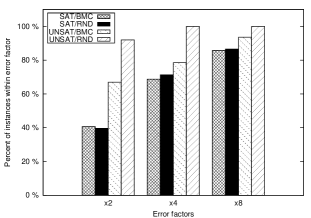
(a) After 2000 backtracks

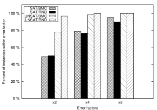
(b) After 35000 backtracks

Figure 1: Quality of prediction, without restarts, for the $rand$ and $bmc$ datasets.

We queried our predictor at different points of the search, ranging from 2000 to 50000 backtracks. Comparisons of the performance of LMP for the rand and bmc data set are presented in Figure 1. Satisfiable problems are harder to predict for both $rand$ and $bmc$ datasets, due to the abrupt way in which search terminates with open nodes.

3.2 Search With Restarts

With restarts, we have to use smaller observation windows to give a prediction early in search as many early restarts are too small. Figure 2 compares the quality of prediction of LMP for the 3 different datasets.

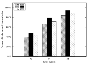
(a) $sat$

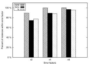
(b) $unsat$

Figure 2: Quality of prediction for the 3 different datasets when using restarts (after 2000 backtracks in the query restart)

The quality of estimates improves with the $bmc$ data set when restarts are enabled. We conjecture this is a result of restarts before the observation window reducing noise.

In order to see if predictions from previous restarts improve the quality of prediction, we opened an observation window at every restart. The window size is $max(1000,0.01\cdot s)$ and starts after a waiting period of $max(500,0.02\cdot s)$, when $s$ is the size of the current restart. At the end of each observation window, two feature vectors were created. The first $\left(x_{r}\right)$ holds all features from Table 1, while the second $\left(\hat{x}_{r}\right)$ is defined as $\hat{x}_{r}=\left\{x_{r}\right\}\cup\left\{f_{w_{1}}\left(x_{1}\right),f_{\hat{w}_{2}}\left(\hat{x}_{2}\right),\dots,f_{\hat{w}_{r-1}}\left(\hat{x}_{r-1}\right)\right\}$. Figure 3 compares the two methods. We see that predictions from earlier restarts improve the quality of later predictions but not greatly.

(a) $sat$

(b) $unsat$

Figure 3: The effect of using predictions from previous restarts. We compare the quality of prediction, through restarts, using two datasets ($bmc$,$rand$). The plots represent the percentage of instances within a factor of 2 from the correct size.

3.3 Solver selection using LMP

In our final experiment, we used these estimations of search cost to improve solver performance. We used two different versions of MiniSat. Solver $A$ used the default MiniSat setting (geometrical factor of 1.5), while solver $B$ used a geometrical factor of 1.2. The challenge is to select which is faster at solving a problem instance.

Table 2 describes the percentage improvement achieved by each of the following strategies. All values are fractions of the cost of solving the entire dataset, picking a solver randomly for each problem, with equal probability. Hence, for each dataset, $average(A,B)=1$:

• best: Use an oracle to indicate which solver will solve the problem faster ($min(A,B)$).

• LMP (oracle): Use both solvers until each reaches the end of its observation window and generate a prediction, using two different models for $sat$ and $unsat$. Use a satisfiability oracle to indicate which model should be queried. Terminate the solver that is predicted to be worse.

• LMP (two models): Use both solvers until each reaches the end of its observation window and generate a prediction, using two different models for $sat$ and $unsat$. Query both models and use the geometric mean as the prediction. Terminate the solver that is predicted to be worse.

These results show that for satisfiable problems, where solver performance varies most, our method reduces the total cost. For unsatisfiable problems, where solver performance does not vary as much, our method does not improve search cost. However, as performance does not change significantly on unsatisfiable instances, the overall impact of our method on satisfiable and unsatisfiable problems is positive.

Table 2: Improvement in total search cost using different schemes

Dataset		Best	LMP (oracle)	LMP(two models)
$rand$	sat	0.591	0.930	0.895
	unsat	0.925	1.009	1.014
$fv$	sat	0.333	0.828	0.832
	unsat	0.852	1.006	1.033
$bmc$	sat	0.404	0.867	0.864
	unsat	0.828	0.997	1.004

References

- [1] Aloul, F., Sierawski, B., Sakallah, K.: Satometer: How much have we searched? In Design Automation Conf.,IEEE (2002) 737-742.
- [2] Een, N., Sorensson, N.: An extensible SAT-solver. Theory and Applications of Satisfiability Testing, (2003), 502-518
- [3] Haim, S., Walsh, T.: SAT Solving Cost Estimation using Online Techniques, Technical Report 0805, UNSW, Australia, February 2008
- [4] Horvitz, E., Ruan, Y., Gomes, C., Kautz, H., Selman, B., Chickering, M.: A Bayesian approach to tackling hard computational problems. Proc. the 17th Conf. on Uncertainty in Artificial Intelligence (UAI-2001), (2001)
- [5] Kilby, P., Slaney, J., Thi baux, S., Walsh, T.: Estimating Search Tree Size. Proc. of the 21st National Conf. of Artificial Intelligence, AAAI, (2006)
- [6] Kokotov, D., Shlyakhter, I. Progress bar for sat solvers. Unpublished manuscript, http://sdg.lcs.mit.edu/satsolvers/progressbar.html. 2000.
- [7] Leyton-Brown, K., Nudelman, E., Shoham, Y.: Learning the Empirical Hardness of Optimization Problems: The Case of Combinatorial Auctions. Proc. of the 8th Int. Conf. on Principles and Practice of Constraint Programming, Springer-Verlag, (2002) 556-572
- [8] Samulowitz, H., Memisevic, R.: Learning to Solve QBF. In Proc. of 22nd Conf. on Artificial Intelligence (AAAI 07), (2007)
- [9] Xu, L., Hoos, H.H., Leyton-Brown, K.: Hierarchical Hardness Models for SAT Principles and Practice of Constraint Programming, (2007), 696-711