Continuum-mechanical, Anisotropic Flow model for polar ice masses, based on an anisotropic Flow Enhancement factor

Abstract

Cont. Mech. Thermodyn. 22 (3), 221–237 (2010). doi: 10.1007/s00161-009-0126-0
Authors’ version; original publication available at www.springerlink.com

A complete theoretical presentation of the Continuum-mechanical, Anisotropic Flow model, based on an anisotropic Flow Enhancement factor (CAFFE model) is given. The CAFFE model is an application of the theory of mixtures with continuous diversity for the case of large polar ice masses in which induced anisotropy occurs. The anisotropic response of the polycrystalline ice is described by a generalization of Glen’s flow law, based on a scalar anisotropic enhancement factor. The enhancement factor depends on the orientation mass density, which is closely related to the orientation distribution function and describes the distribution of grain orientations (fabric). Fabric evolution is governed by the orientation mass balance, which depends on four distinct effects, interpreted as local rigid body rotation, grain rotation, rotation recrystallization (polygonization) and grain boundary migration (migration recrystallization), respectively. It is proven that the flow law of the CAFFE model is truly anisotropic despite the collinearity between the stress deviator and stretching tensors.

1 Introduction

In order to study the mechanical behaviour of large polar ice masses, we use the method of continuum mechanics. Generally, ice is treated as an incompressible, isotropic and extremely viscous non-Newtonian fluid, and Glen’s flow law (Glen 1955, Nye 1952) is used as a constitutive equation. However, for thick polar ice masses anisotropic behaviour occurs, and therefore, Glen’s flow law must be changed. Many efforts have been undertaken to deal with this problem (e.g. Hutter 1983, Budd and Jacka 1989, Jacka and Budd 1989, Azuma 1995, Staroszczyk and Morland 2001, Morland and Staroszczyk 2003, Placidi et al. 2006, Gagliardini et al. 2009). In this paper we will present a continuum-mechanical model, which is based on earlier work by Faria (2001, 2006a, 2006b), Placidi (2004, 2005), Placidi et al. (2004), Placidi and Hutter (2006a, b). The model is referred to as the Continuum-mechanical, Anisotropic Flow model, based on an anisotropic Flow Enhancement factor, or “CAFFE model” for short.

The macroscopic anisotropy of polar ice is due to its microstructure. Ice is a polycrystalline material made of a vast number of crystallites (grains), the mechanical behaviour of which is extremely anisotropic (Jacka and Budd 1989). A single ice crystal shows transversely isotropic behaviour, and its $c$-axis (optical axis) defines the privileged direction (Boehler 1987). Slide along basal planes, orthogonal to the $c$-axis, is easier than slide along other crystallographic planes, and since the study by McConnel (1891) it has been common to refer to this as the deck-of-cards behaviour of ice. However, the transition from the mechanics of a single crystal to that of a huge polycrystal entails the complication of different deformation mechanisms, and the selection of these mechanisms in different situations. A continuum approach is deemed appropriate in order to deal with this problem in a manageable fashion. We choose the approach of describing the polycrystalline ice as a mixture (Truesdell 1957a, b), the species of which are the grains characterized by a certain orientation (Faria et al. 2006). The orientations of the crystallites, i.e., the unit vectors parallel to the $c$-axes, belong to a continuous space, so that the ice is considered a Mixture with Continuous Diversity (MCD) (Faria 2001).

In the MCD theory, equations are defined at the species level (“microscopic”) and at the mixture level (“macroscopic”). However, the “microscopic” equations do not govern the evolution of single crystallites, the dynamics of which is hidden in the theory. The objective of the mixture approach is to predict the polycrystalline behaviour only. In other words, the CAFFE model is a macroscopic model, and the microstructure is taken into account only phenomenologically, without going down to the actual microscopic level. The same holds for classical continuum mechanics: we know that matter is discontinuous, spaces between particles (atoms, molecules, etc.) are empty and the molecular structures have strong influences on the mechanical behaviour. However, the microstructural characteristics are not resolved in detail; instead, constitutive equations for a continuous body are postulated that are in accordance with experimental data and general principles like determinism, objectivity and the Second Law of Thermodynamics. In the same way, in a MCD, the behaviour of a single species is important for the mixture dynamics, but single species dynamics does not correspond to any measurable quantity.

The general set of equations for polycrystalline ice modelled as a MCD was developed by Faria (2001, 2006a), Faria et al. (2006), Faria (2006b), Placidi and Hutter (2006b), and restrictions of the constitutive equations due to the Second Law of Thermodynamics were given by these authors. Placidi (2004, 2005), Placidi and Hutter (2006a) suggested explicit forms for the constitutive relations. In this study, we present the CAFFE model as an improved version of these previous formulations. After defining the notation (Section 2), we derive in Section 3 in a rational way the set of CAFFE equations, while taking care that the following requirements are satisfied:

• All fundamental principles of classical continuum mechanics must be fulfilled.

• The model must be sufficiently simple to allow numerical implementation in current flow models for polar ice masses.

• The parameters of the model must in principle be measurable by either laboratory experiments or field observations.

In Section 3.1, we define the orientation mass density, and in Section 3.2 we deal with the general mass balance that governs its evolution. In Section 3.3, we characterize the constitutive quantities introduced in Section 3.2 in order to describe grain rotation, local rigid body rotation, grain boundary migration (or migration recrystallization) and polygonization (or rotation recrystallization). In Sections 3.4 and 3.5, we present an anisotropic generalization of Glen’s flow law based on a scalar anisotropic enhancement factor. It is similar to that by Placidi and Hutter (2006a), but simpler and consistent with the Second Law of Thermodynamics.

Section 4 is devoted to the analysis of the anisotropic properties of the CAFFE flow law. We note the collinearity between the stretching and the stress deviator tensors and show that collinearity and isotropy do not share any fundamental concepts, in the sense that non-collinear, isotropic flow laws as well as collinear, anisotropic flow laws are possible (e.g. Liu 2002, Faria 2008). A discussion of the advantages and disadvantages of collinearity in an anisotropic flow law terminates Section 4.

Some examples for the constitutive relations introduced in Section 3.3 are provided in the appendix (Section A).

2 Notation

For a general field $A$, the star superscript $A^{\ast}$ denotes an orientational dependence $A^{\ast}\left(\mathbf{x},t,\mathbf{n}\right)$, where $t$ is the time, $\mathbf{x}$ the position vector and $\mathbf{n}$ the orientation (unit vector parallel to the $c$-axis) in the present configuration. Otherwise the field $A\left(\mathbf{x},t\right)$ is supposed to be independent of $\mathbf{n}$. It is implicitly assumed that for a given position $\mathbf{x}$ all possible orientations $\mathbf{n}$ are defined. The gradient ($\nabla$) and divergence ($\nabla\cdot$) operators are applied, as usual, to the space variable $\mathbf{x}$, while the orientational gradient ($\nabla^{\ast}$) and divergence ($\nabla^{\ast}\cdot$) operators are applied to the orientational variable $\mathbf{n}$. For arbitrary scalars $A^{\ast}$ and vectors $\mathbf{A}^{\ast}$, we define

$$\nabla A^{\ast}=\mbox{$\displaystyle\frac{\partial A^{\ast}}{\partial\mathbf{x}}$}\,, \nabla^{\ast}A^{\ast}=\mbox{$\displaystyle\frac{\partial A^{\ast}}{\partial\mathbf{n}}$}-\left(\mbox{$\displaystyle\frac{\partial A^{\ast}}{\partial\mathbf{n}}$}\cdot\mathbf{n}\right)\mathbf{n}\,,$$ (1)

$$\nabla\cdot\mathbf{A}^{\ast}=\mathrm{tr}\left[\nabla\mathbf{A}^{\ast}\right]=\mathrm{tr}\left[\mbox{$\displaystyle\frac{\partial\mathbf{A}^{\ast}}{\partial\mathbf{x}}$}\right]\,, \nabla^{\ast}\cdot\mathbf{A}^{\ast}=\mathrm{tr}\left[\mbox{$\displaystyle\frac{\partial\mathbf{A}^{\ast}}{\partial\mathbf{n}}$}-\left(\mbox{$\displaystyle\frac{\partial\mathbf{A}^{\ast}}{\partial\mathbf{n}}$}\cdot\mathbf{n}\right)\,\mathbf{n}\right]\,.$$ (2)

An immediate consequence of Eq. (1)₂ is $\nabla^{\ast}A^{\ast}\cdot\mathbf{n}=0$. We also note that the explicit form of the orientational gradient operator in spherical coordinates is

$$\nabla^{\ast}A^{\ast} = \mathbf{e}_{1}\left[\cos\theta\cos\varphi\mbox{$\displaystyle\frac{\partial A^{\ast}}{\partial\theta}$}-\mbox{$\displaystyle\frac{\sin\varphi}{\sin\theta}$}\mbox{$\displaystyle\frac{\partial A^{\ast}}{\partial\varphi}$}\right]$$ (3)

$$+ \mathbf{e}_{2}\left[\cos\theta\sin\varphi\mbox{$\displaystyle\frac{\partial A^{\ast}}{\partial\theta}$}+\mbox{$\displaystyle\frac{\cos\varphi}{\sin\theta}$}\mbox{$\displaystyle\frac{\partial A^{\ast}}{\partial\varphi}$}\right]+\mathbf{e}_{3}\left[-\sin\theta\mbox{$\displaystyle\frac{\partial A^{\ast}}{\partial\theta}$}\right]\,,$$

where $\left\{\mathbf{e}_{1},\mathbf{e}_{2},\mathbf{e}_{3}\right\}$ is a fixed orthonormal basis on which we project vectors and tensors, and $\theta$ and $\varphi$ are the zenith and azimuth angle, respectively. The orientation $\mathbf{n}$ can be parameterized as follows,

$$\mathbf{n}=\left(\begin{array}[]{c}\sin\theta\cos\varphi\\ \sin\theta\sin\varphi\\ \cos\theta\end{array}\right)=\sin\theta\cos\varphi\,\,\mathbf{e}_{1}+\sin\theta\sin\varphi\,\,\mathbf{e}_{2}+\cos\theta\,\,\mathbf{e}_{3}\,.$$ (4)

3 CAFFE model

3.1 Orientation mass density, orientation distribution function

In the CAFFE model, each point of the continuous body is interpreted as a representative volume element of the polycrystal that encloses a large number of crystallites with their own orientations. Each orientation is represented by a unit vector $\mathbf{n}\in\mathcal{S}^{2}$ (where $\mathcal{S}^{2}$ denotes the unit sphere) parallel to the $c$-axis (Fig. 1a).

Figure 1: (a) Each point of the unit sphere $\mathcal{S}^{2}$ represents a particular orientation $\mathbf{n}$. The orientation transition rate $\mathbf{u}^{\ast}$ is orthogonal to $\mathbf{n}$. Panel (b) shows a projection on the plane spanned by $\mathbf{u}^{\ast}$ and $\mathbf{n}$. The anticlockwise direction of the rotation corresponds to a spin velocity $\mathbf{s}^{\ast}$ pointing out of the plane.

In the MCD framework, distributions of continuous species parameters (like the orientation) are expressed in terms of associated mass densities. This means that for every time $t$ and position $\mathbf{x}$ an orientation mass density $\varrho^{\ast}\left(\mathbf{x},t,\mathbf{n}\right)$ is defined such that, when integrated over $\mathcal{S}^{2}$, the usual mass density of the polycrystal $\varrho\left(\mathbf{x},t\right)$ results,

$$\varrho\left(\mathbf{x},t\right)=\int\limits_{\mathcal{S}^{2}}\!\varrho^{\ast}\left(\mathbf{x},t,\mathbf{n}\right)\,\mathrm{d}^{2}n\,,$$ (5)

where $\mathrm{d}^{2}n$ ($=\sin{\theta}\,\mathrm{d}\theta\,\mathrm{d}\varphi$ in spherical coordinates) is the solid angle increment on the unit sphere $\mathcal{S}^{2}$. The orientation mass density $\varrho^{\ast}$, as stated in Eq. (5), has the following physical meaning: the product $\varrho^{\ast}\!\left(\mathbf{x},t,\mathbf{n}\right)\,\mathrm{d}^{2}n$ is the mass fraction of crystallites with orientations directed towards $\mathbf{n}$ within the solid angle $\mathrm{d}^{2}n$. Therefore, the quantity $\varrho^{\ast}/\varrho$ can be interpreted as the analogue of the usual orientation distribution function (ODF) (e.g. Rashid 1992, Placidi and Hutter 2004), which is also used in the context of liquid crystals (e.g. Blenk et al. 1992, Papenfuss 2000) or in mesoscopic damage mechanics (e.g. Massart et al. 2004, Papenfuss and Van 2008). However, we remark that in the glaciological community, the ODF usually describes the relative number, and not the mass fraction, of grains with a certain orientation.

3.2 Orientation mass balance

Some kinematic quantities are required in order to describe the evolution of positions and orientations. We will use the classical velocity $\mathbf{v}\left(\mathbf{x},t\right)$ and the orientation transition rate $\mathbf{u}^{\ast}\left(\mathbf{x},t,\mathbf{n}\right)$ as kinematic rates. The velocity $\mathbf{v}$ represents the transition of mass from a given position to a neighbouring position in three-dimensional space. Analogously, the orientation transition rate $\mathbf{u}^{\ast}$ represents the transition of mass from a certain orientation to a neighbouring orientation on the unit sphere. Note that the velocity is assumed to be independent on the orientation, while the orientation transition rate can depend on the orientation [for a longer discussion on this topic see e.g. Faria (2006a)].

As shown by Faria (2001), the normality condition $\mathbf{n}\cdot\mathbf{n}=1$ makes the orientation transition rate $\mathbf{u}^{\ast}$ orthogonal to $\mathbf{n}$ ($\mathbf{u}^{\ast}\cdot\mathbf{n}=0$) and to the spin velocity $\mathbf{s}^{\ast}$ of the crystallites ($\mathbf{u}^{\ast}=\mathbf{s}^{\ast}\times\mathbf{n}$); see also the caption of Fig. 1b. In the MCD theory, the balance of mass is formulated as

$$\mbox{$\displaystyle\frac{\partial\varrho^{\ast}}{\partial t}$}+\nabla\cdot\left[\varrho^{\ast}\mathbf{v}\right]+\nabla^{\ast}\cdot\left[\varrho^{\ast}\mathbf{u}^{\ast}\right]=\varrho^{\ast}\Gamma^{\ast}\,.$$ (6)

The quantity $\Gamma^{\ast}$ is the specific mass production rate. It describes the rate of change of mass (per unit mass) of one species (for crystallites having a certain orientation $\mathbf{n}$) into another species with a different orientation. This corresponds physically to the effect of grain boundary migration (migration recrystallization).

Integration of Eq. (6) over the unit sphere $\mathcal{S}^{2}$ gives the balance of mass of the polycrystal,

$$\mbox{$\displaystyle\frac{\partial\varrho}{\partial t}$}+\nabla\cdot[\varrho\mathbf{v}]=0\,,$$ (7)

provided that Eq. (5) and

$$\int_{\mathcal{S}^{2}}\varrho^{\ast}\Gamma^{\ast}\,\mathrm{d}^{2}n=0,\qquad\int_{\mathcal{S}^{2}}\nabla^{\ast}\cdot[\varrho^{\ast}\mathbf{u}^{\ast}]\,\mathrm{d}^{2}n=0$$ (8)

hold. Note that Eq. (8)₁ describes the conservation of mass, and Eq. (8)₂ is a consequence of the Gauss theorem.

3.3 Constitutive equations for the orientation mass balance

Placidi and Hutter (2006b) showed that the orientation transition rate $\mathbf{u}^{\ast}$ can be decomposed into two parts,

$$\mathbf{u}^{\ast}=\mathbf{u}^{\ast}_{\mathrm{rbr}}+\mathbf{u}^{\ast}_{\mathrm{c}}=\mathbf{W}\cdot\mathbf{n}+\mathbf{u}^{\ast}_{\mathrm{c}}\,,$$ (9)

where $\mathbf{u}^{\ast}_{\mathrm{rbr}}=\mathbf{W}\cdot\mathbf{n}$ is the contribution of the local rigid body rotation of the polycrystal, $\mathbf{W}=\mathrm{Skw}\,\mathbf{L}$ is the skew-symmetric part of the velocity gradient $\mathbf{L}=\nabla\mathbf{v}$ and $\mathbf{u}^{\ast}_{\mathrm{c}}$ is a vector to be constitutively prescribed. For the latter, we introduce phenomenologically a further decomposition,

$$\mathbf{u}_{\mathrm{c}}^{\ast}=\mathbf{u}^{\ast}_{\mathrm{gr}}+\frac{\mathbf{q}^{\ast}}{\varrho^{\ast}}\,,$$ (10)

in order to separate the physical effects of (i) grain rotation (“deck-of-cards effect”, see also Fig. 2), to be modelled by $\mathbf{u}^{\ast}_{\mathrm{gr}}$, and (ii) rotation recrystallization (polygonization), to be modelled by the orientation flux $\mathbf{q}^{\ast}$ (Gödert 2003).

Figure 2: Schematic, two-dimensional representations of representative volume elements. Straight arrows inside the volume elements show $c$-axes of crystallites well oriented for deformation. Curved arrows indicate the rotational motion of such crystallites due to grain rotation (“deck-of-cards effect”). Arrows outside the volume elements mark the state of stretching. In case (a), the state of stretching is pure shear. The $c$-axes are well oriented at angles of $45^{\circ}$ with respect to the axes of extension and compression, and the $c$-axes rotate towards the axis of compression and away from the axis of extension. Case (b) shows the same configuration rotated anticlockwise by $45^{\circ}$ (rotated pure shear) for two equivalent volume elements.

By assuming a linear dependence on the stretching tensor $\mathbf{D}=\mathrm{Sym}\,\mathbf{L}$, the constitutive vector $\mathbf{u}^{\ast}_{\mathrm{gr}}$ takes the form

$$\mathbf{u}^{\ast}_{\mathrm{gr}}=\iota\,[((\mathbf{D}\cdot\mathbf{n})\cdot\mathbf{n})\mathbf{n}-\mathbf{D}\cdot\mathbf{n}]\,,$$ (11)

where $\iota>0$ is a material parameter [$\iota$ is called “shape factor” in the theory of rotational diffusion; see e.g. Faria (2001)]. Dafalias (2001) noted that, for the special case $\iota=1$, the unit vector $\mathbf{n}$ remains orthogonal to the associated material area element, and thus the rotation is an affine rotation. However, the possibility of non-affine rotations cannot a priori be ruled out. An advantage of the present macroscopic approach is the possibility to parameterize $\iota$ without any conflicts with “microscopic” assumptions. [As a contrasting example, the model by Staroszczyk and Morland (2001) is also a macroscopic model, but it is restricted to affine rotations.] In fact, Placidi (2004) showed that the fabrics in the upper 2000 m of the GRIP ice core in central Greenland can be best explained by the value $\iota\approx{}0.4$. A study on the EPICA ice core in Dronning Maud Land, East Antarctica, provided a best fit between modelled and measured fabrics for $\iota=0.6$ (Seddik et al. 2008).

The constitutive equations (9) and (11) are not new in the literature and not specific to ice (e.g. Larson 1988, Blenk et al. 1992, Larson 1999, Papenfuss 2000, Dafalias 2001, and references therein). They were derived by Placidi (2004) within the MCD framework. We remark that, even though the unit vector $\mathbf{n}$ specifying the orientation of the crystals is unique, Eq. (11) is not the most general case. In fact, Dafalias (2001) discussed the case of non-affine rotations. More generally, Faria (2001) and Placidi and Hutter (2006b) derived the thermodynamically consistent class of these constitutive equations.

Following the argumentation by Gödert (2003), the orientation flux (which is supposed to describe rotation recrystallization) is modelled as a diffusive process,

$$\mathbf{q}^{\ast}=-\lambda\,\nabla\!^{\ast}[\rho^{\ast}\mathcal{H}^{\ast}]\,,$$ (12)

where the parameter $\lambda>0$ is the orientation diffusivity, and $\mathcal{H}^{\ast}$ is an orientation-dependent “hardness” function. However, recent results by Durand et al. (2008) suggest that rotation recrystallization is an isotropic process not affected by the orientation. In this case, the choice

$$\mathcal{H}^{\ast}\equiv 1$$ (13)

is indicated, which renders Eq. (12) equivalent to Fick’s laws of diffusion on the unit sphere. We remark that in the MCD theory the hardness function is called the chemical potential for the given species. It is a constitutive quantity that depends at least on the OMD $\varrho^{\ast}$. Consequently, it is possible to show by applying the chain rule that often an equivalent of Fick’s law results even when $\mathcal{H}^{\ast}$ is not a constant (e.g. Faria 2001).

As for the specific mass production rate $\Gamma^{\ast}$, in the studies by Placidi (2004) and Placidi (2005) it was shown that, in order to model the effect of grain boundary migration, a reasonable constitutive equation for $\Gamma^{\ast}$ is

$$\Gamma^{\ast}=\hat{\Gamma}\left[D^{\ast}-\langle D^{\ast}\rangle\right]\,.$$ (14)

The dimensionless quantity $D^{\ast}$ is called the stretching deformability of crystallites,

$$D^{\ast}\equiv 5\,\frac{(\mathbf{D}\cdot\mathbf{n})^{2}-\left((\mathbf{D}\cdot\mathbf{n})\cdot\mathbf{n}\right)^{2}}{\mathrm{tr}\left(\mathbf{D}^{2}\right)}\,;$$ (15)

its physical meaning is the square of the resolved shear strain rate (or stretching) on the basal plane, normalized by the orientation-independent scalar invariant $\mathrm{tr}(\mathbf{D}^{2})$. The additional factor $5$ is merely a convention, for which the reason will become clear below (Section 3.4). Further, $\langle\cdot\rangle$ is the averaging operator

$$\langle\cdot\rangle\equiv\int_{\mathcal{S}^{2}}\frac{\varrho^{\ast}}{\varrho}\,\left(\cdot\right)\,\mathrm{d}^{2}n\,,$$ (16)

and $\hat{\Gamma}$ is a constitutive parameter (see Fig. 3). The conservation of mass expressed by Eq. (8)₁ is compatible with Eqs. (14)–(16), and they are also compatible with the rational constitutive theory developed by Placidi and Hutter (2006b). Provided that $\hat{\Gamma}>0$, Eqs. (14)–(16) have the effect that $\Gamma^{\ast}$ is greater than zero when the stretching deformability $D^{\ast}$ is high, and $\Gamma^{\ast}$ is less than zero when the stretching deformability $D^{\ast}$ is low. This means that crystallites well-oriented for deformation will be enlarged (e.g. Kamb 1972). Since ice crystallites deform essentially by basal shearing, the resolved shear rate (which is proportional to the orientation dependence of $D^{\ast}$) is related to the rate of accumulation of deformation energy in the material, which drives dynamic recrystallization.

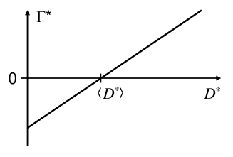
Figure 3: Specific mass production rate $\Gamma^{\ast}$ according to Eq. (14).

The first contribution in Eq. (9), $\mathbf{u}^{\ast}_{\mathrm{rbr}}$, is thermodynamically reversible, because there is no energy dissipation associated with local rigid body rotations. The second contribution, $\mathbf{u}^{\ast}_{\mathrm{c}}$, has been split up in Eq. (10) into $\mathbf{u}^{\ast}_{\mathrm{gr}}$ and $\mathbf{q}^{\ast}$. The grain-rotation part, $\mathbf{u}^{\ast}_{\mathrm{gr}}$, is thermodynamically irreversible because it is linearly dependent on the stretching tensor $\mathbf{D}$, see Eq. (11), which by definition must vanish for any reversible process in a viscous fluid (e.g., Hutter 1983, Müller 1985, Faria 2001). The rotation-recrystallization part, $\mathbf{q}^{\ast}$, is thermodynamically irreversible because of the diffusive nature of the process as specified in Eq. (12). The specific mass production rate $\Gamma^{\ast}$ is also thermodynamically irreversible, because grain growth and recrystallization are thermally activated, irreversible processes [see also the discussion by Faria et al. (2006, Sect. 3c)]. Note that, besides the physical interpretation, the thermodynamic reversibility or irreversibility of these terms can also be investigated by exploiting the Second Law of Thermodynamics (Faria 2006a, Placidi and Hutter 2006b).

A problem is that it is not possible at the moment to constrain the values of the two parameters $\hat{\Gamma}$ and $\lambda$ in a reasonable fashion. Determining these parameters by experiments is very difficult, because the relevant time scales are far too large and the strain rates far too low to be reproduced in the laboratory. Deformation experiments, even if conducted over a period of years, inevitably end up by activating non-natural deformation and recrystallization mechanisms. The only promising way out of this is to measure the fabrics ($c$-axis distributions) and the changes in grain stereology (sizes and shapes) in natural polar ice and fit $\hat{\Gamma}$ and $\lambda$ to these observations. The situation is complicated further by the fact that a functional dependence of these parameters on temperature and/or dislocation density should be considered (cf. Faria 2006a, b). This requires further attention.

Some examples for the orientation transition rate (grain rotation) and the orientation production rate (recrystallization) under different deformation regimes are given in the appendix (Section A).

3.4 Anisotropic flow law

The anisotropic flow law presented by Placidi and Hutter (2006a) has been modified in order to make it simpler and compatible with the Second Law of Thermodynamics,

$$\mathbf{D}=A\,\hat{E}(S)\left(\frac{\mathrm{tr}(\mathbf{S}^{2})}{2}\right)^{(n-1)/2}\mathbf{S}\,,$$ (17)

where $A$ and $n$ are the same rate factor and stress exponent, respectively, as in the isotropic Glen flow law, $\mathbf{S}$ is the stress deviator defined by

$$\mathbf{S}=\mathbf{t}-\left(\frac{\mathrm{tr}\,\mathbf{t}}{3}\right)\,\mathbf{I}$$ (18)

(i.e., the deviatoric part of the Cauchy stress tensor $\mathbf{t}$) and $\mathbf{I}$ is the identity tensor. Further, $S\in{}[0,\,5/2]$ is the positive scalar

$$S=\langle S^{\ast}\rangle=\int_{\mathcal{S}^{2}}\frac{\varrho^{\ast}}{\varrho}\,S^{\ast}\,\mathrm{d}^{2}n\,,$$ (19)

and $S^{\ast}$ is the analogue of $D^{\ast}$,

$$S^{\ast}\equiv 5\,\frac{(\mathbf{S}\cdot\mathbf{n})^{2}-\left((\mathbf{S}\cdot\mathbf{n})\cdot\mathbf{n}\right)^{2}}{\mathrm{tr}(\mathbf{S}^{2})}\,,$$ (20)

which can also be written in terms of the Cauchy stress tensor as

$$S^{\ast}=5\,\frac{((\mathbf{t}\cdot\mathbf{n})\times\mathbf{n})^{2}}{\mathrm{tr}(\mathbf{t}^{2})}>0\,.$$ (21)

We call $S^{\ast}$ the stress deformability of crystallites and $S$ the stress deformability of the polycrystal. In the literature, the scalar $(\mathbf{t}\cdot\mathbf{n})^{2}-\left((\mathbf{t}\cdot\mathbf{n})\cdot\mathbf{n}\right)^{2}=(\mathbf{S}\cdot\mathbf{n})^{2}-\left((\mathbf{S}\cdot\mathbf{n})\cdot\mathbf{n}\right)^{2}$ has been identified with the square of the resolved stress on the basal plane, so that the stress deformability of crystallites, Eq. (20), can also be called the normalized square of the resolved stress on the basal plane. As for the stress exponent, it is often chosen as $n=3$ (e.g. Paterson 1994), but we will keep it general in the following.

For a thermodynamicist it may appear strange to formulate a constitutive equation in terms of the stretching tensor and not in terms of the stress deviator. However, there is no inconsistency in this formulation. From the theoretical point of view the stress is indeed the constitutive property and the strain rate (stretching) is the variable, but whether we choose this or the inverse relation is just a matter of taste or custom. In the glaciological community the inverse form is most commonly used; in the book by Hutter (1983) the historical reason for this is given.

Our new formulation of the flow law is not only compatible with the Second Law of Thermodynamics (Placidi and Hutter 2006b), but Eq. (17) is much more flexible than the previous Placidi–Hutter formulation. The mechanical non-linearity $\left(\mathrm{tr}(\mathbf{S}^{2})/2\right)^{(n-1)/2}$ and the anisotropic part $\hat{E}(S)$ are now nicely separated, so that the choice of the stress exponent is not limited to $n=3$ any more, and the new formulation is not even restricted to a power law.

In Section 3.5 we will show that, due to Eq. (17), the two quantities $D^{\ast}$ and $S^{\ast}$ defined in Eqs. (15) and (20) are identical,

$$S^{\ast}=D^{\ast}\,,$$ (22)

so that we will simply call them the species (or “crystallite”) deformability. In the same way, the positive scalars $S$ and $D$ will be called the polycrystal deformability,

$$S=\langle S^{\ast}\rangle=\langle D^{\ast}\rangle=D\,.$$ (23)

Both the crystal and polycrystal deformabilities can only assume values in the range from zero to 5/2,

$$S^{\ast}=D^{\ast}\in[0,\,\mbox{$\frac{5}{2}$}]\,,\quad S=D\in[0,\,\mbox{$\frac{5}{2}$}]\,.$$ (24)

The proof (which is laborious and shall not be detailed here) involves to insert Eq. (4) in Eqs. (15) and (16), and study the maxima and minima of the deformabilities $D^{\ast}$ and $D$ for general stretching tensors $\mathbf{D}$ as functions of the zenith angle $\theta$ and the azimuth angle $\phi$. Taking into account that for a randomly distributed OMD (isotropic fabric)

$$\varrho^{\ast}=\frac{\varrho}{4\pi}\quad\Rightarrow\quad S=D=1$$ (25)

holds, the function $\hat{E}(S)$ is demanded to be monotone, of class $C^{1}[0,\,5/2]$ and has the fixed points

$$\hat{E}(0)=E_{\mathrm{min}}\,,\qquad\hat{E}(1)=1\,,\qquad\hat{E}(\mbox{$\frac{5}{2}$})=E_{\mathrm{max}}\,,$$ (26)

where $E_{\mathrm{min}}<1$ and $E_{\mathrm{max}}>1$ are the minimum and the maximum enhancement factors. This means that if the polycrystal deformability $S$ is highest ($S=5/2$), the flow law (17) gives the maximum stretching, if the polycrystal deformability $S$ is lowest ($S=0$), the flow law (17) gives the minimum stretching, and if the polycrystal deformability is the same as for the isotropic case ($S=1$), the flow law (17) reproduces the classical Glen flow law.

As for the detailed functional form of the anisotropic enhancement factor $\hat{E}(S)$, some experimental data suggest that the enhancement factor depends on the “averaged Schmid factor” to the fourth power (Azuma 1995, Miyamoto 1999). Since the polycrystal deformability $S$ of the CAFFE model is related to the square of the averaged Schmidt factor, it is reasonable to assume a dependency of $\hat{E}$ on $S^{2}$. However, this does not allow to fulfill Eq. (26) for arbitrary choices of the parameters $E_{\mathrm{min}}$ and $E_{\mathrm{max}}$. Hence the function $\hat{E}(S)$ is chosen to depend on $S^{2}$ in the interval $[1,\,5/2]$ [in which the experiments by Azuma (1995) and Miyamoto (1999) have been carried out] only, and for the interval $[0,1]$ a dependency on $S^{\tau}$ is introduced. The exponent $\tau$ is adjusted such that the function is continuously differentiable at $S=1$. This yields

$$\hat{E}\left(S\right)=\left\{\begin{array}[]{lr}\left(1-E_{\mathrm{min}}\right)S^{\tau}+E_{\mathrm{min}}\,,\qquad\tau=\mbox{$\displaystyle\frac{8}{21}$}\left(\mbox{$\displaystyle\frac{E_{\mathrm{max}}-1}{1-E_{\mathrm{min}}}$}\right)\,,&S\in\left[0,1\right]\,,\vspace{1mm}\\ \mbox{$\displaystyle\frac{4S^{2}\left(E_{\mathrm{max}}-1\right)+25-4E_{\mathrm{max}}}{21}$}\,,&S\in\left[1,\frac{5}{2}\right]\,.\end{array}\right.$$ (27)

Several investigations (e.g. Russell-Head and Budd 1979, Pimienta et al. 1987, Budd and Jacka 1989) indicate that the parameter $E_{\mathrm{max}}$ (maximum softening) is $\sim{}10$. The parameter $E_{\mathrm{min}}$ (maximum hardening) can be realistically chosen between 0 and $\sim{}0.1$, a non-zero value serving mainly the purpose of avoiding numerical problems. The function (27) is shown in Fig. 4.

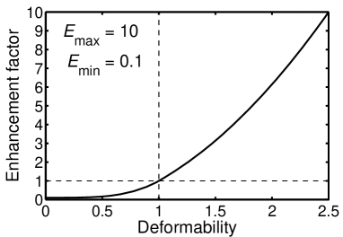
Figure 4: Anisotropic enhancement factor $\hat{E}(S)$ as a function of the deformability $S$ according to Eq. (27), for $E_{\mathrm{max}}=10$ and $E_{\mathrm{min}}=0.1$.

3.5 Inversion of the anisotropic flow law

The anisotropic flow law (17) can be inverted analytically as long as the power-law form is retained. From Eq. (17) we find

$$\frac{\mathrm{tr}(\mathbf{D}^{2})}{2}=A^{2}\,\hat{E}^{2}(S)\left(\frac{\mathrm{tr}(\mathbf{S}^{2})}{2}\right)^{n-1}\frac{\mathrm{tr}(\mathbf{S}^{2})}{2}\,,$$ (28)

and thus

$$\frac{\mathrm{tr}(\mathbf{S}^{2})}{2}=A^{-2/n}\,\hat{E}^{-2/n}(S)\left(\frac{\mathrm{tr}(\mathbf{D}^{2})}{2}\right)^{1/n}\,.$$ (29)

Inserting this result in Eq. (17) and solving for $\mathbf{S}$ yields

$$\mathbf{S}=A^{-1/n}\,\hat{E}^{-1/n}(S)\,\left(\frac{\mathrm{tr}(\mathbf{D}^{2})}{2}\right)^{-(1-1/n)/2}\mathbf{D}\,.$$ (30)

In order to complete the inversion, we must prove Eqs. (22) and (23). By writing Eq. (17) in short as $\mathbf{D}=\mathbf{S}/(2\eta)$ (where $\eta$ is the shear viscosity of the flow law), we obtain for the crystalline deformability $S^{\ast}$

$$S^{\ast} = 5\,\frac{(\mathbf{S}\cdot\mathbf{n})^{2}-((\mathbf{S}\cdot\mathbf{n})\cdot\mathbf{n})^{2}}{\mathrm{tr}(\mathbf{S}^{2})}$$ (31)

$$= 5\,\frac{(2\eta\mathbf{D}\cdot\mathbf{n})^{2}-((2\eta\mathbf{D}\cdot\mathbf{n})\cdot\mathbf{n})^{2}}{\mathrm{tr}[(2\eta\mathbf{D})^{2}]}$$

$$= 5\,\frac{(\mathbf{D}\cdot\mathbf{n})^{2}-((\mathbf{D}\cdot\mathbf{n})\cdot\mathbf{n})^{2}}{\mathrm{tr}(\mathbf{D}^{2})}\;=\;D^{\ast}\,,$$

so that Eq. (22) is proven. By applying the averaging operator (16) to this result, we find immediately

$$S=D\,,$$ (32)

which is the assertion of Eq. (23). Hence, we can replace $S$ by $D$ in Eq. (30), which yields the inverted anisotropic flow law

$$\mathbf{S}=A^{-1/n}\,\hat{E}^{-1/n}(D)\,\left(\frac{\mathrm{tr}(\mathbf{D}^{2})}{2}\right)^{-(1-1/n)/2}\mathbf{D}\,.$$ (33)

4 On the anisotropy of the CAFFE flow law

In Sections 3.4 and 3.5 we have given the generalization of Glen’s flow law considered in the CAFFE model. The anisotropy of the CAFFE flow law has recently been analyzed mathematically by Faria (2008) through the derivation of the symmetry group of the CAFFE model. In this section, we prove in a more direct way that the CAFFE flow is anisotropic despite the collinearity between the tensors $\mathbf{S}$ and $\mathbf{D}$, and give examples in order to justify this choice.

4.1 CAFFE anisotropy in the context of material theory

In the context of constitutive theory, the definition of isotropy states that any rotation of the body in question does not alter its material response. Mathematically speaking, this means invariance of the material functions (or functionals) to arbitrary orthogonal transformations $\mathbf{P}$ of an undistorted configuration $\kappa$ (e.g. Liu 2002, p. 86), so that the symmetry group $\mathcal{G}$ of the material contains the entire group of orthogonal transformations O(3) [$\mathcal{G}\supseteq{}\mathrm{O(3)}$]. Anisotropy is the logical opposite: for at least one orthogonal transformation the invariance does not hold, so that the symmetry group does not contain the entire group of orthogonal transformations [$\mathcal{G}\not\supseteq{}\mathrm{O(3)}$].

By construction, the anisotropy of the CAFFE flow law (17) must be contained in the enhancement factor $\hat{E}(S)$ via the polycrystal deformability $S$. So let us assume that, at the initial time $t=0$, the initial configuration $\kappa_{t=0}$ is given by an unloaded ice specimen with the OMD $\varrho^{\ast}(\mathbf{x},\mathbf{n},0)$. At $t=0^{+}$, it is subjected to the stress $\mathbf{S}$, and, according to Eqs. (19) and (20), the resulting polycrystal deformability is

$$S=\frac{5}{\varrho\,\mathrm{tr}(\mathbf{S}^{2})}\int_{\mathcal{S}^{2}}\varrho^{\ast}(\mathbf{n})\left[(\mathbf{S}\cdot\mathbf{n})^{2}-((\mathbf{S}\cdot\mathbf{n})\cdot\mathbf{n})^{2}\right]\,\mathrm{d}^{2}n\,,$$ (34)

where, for simplicity of notation and in the rest of this session, we will omit the dependence of OMD on position and time. Now let us consider a second initial configuration $\tilde{\kappa}_{t=0}$ rotated by a proper orthogonal tensor $\mathbf{P}$ with respect to $\kappa_{t=0}$. The rotated orientations are given by

$$\tilde{\mathbf{n}}=\mathbf{P}\cdot\mathbf{n}$$ (35)

(Fig. 5). The OMD follows the rotation, so that

$$\tilde{\varrho}^{\ast}(\tilde{\mathbf{n}})=\varrho^{\ast}(\mathbf{n})\quad\stackrel{{\scriptstyle(\ref{orientation_trafo})}}{{\Rightarrow}}\quad\tilde{\varrho}^{\ast}(\tilde{\mathbf{n}})=\varrho^{\ast}(\mathbf{P}^{\mathrm{T}}\cdot\tilde{\mathbf{n}})\,.$$ (36)

At $t=0^{+}$, the rotated configuration is subjected to the stress $\tilde{\mathbf{S}}$, which is supposed to be the same as before,

$$\tilde{\mathbf{S}}=\mathbf{S}$$ (37)

(Fig. 5). The polycrystal deformability with respect to the rotated configuration is then

$$\tilde{S} \stackrel{{\scriptstyle(\ref{stress_deformability_unrot})}}{{=}} \frac{5}{\varrho\,\mathrm{tr}(\tilde{\mathbf{S}}^{2})}\int_{\mathcal{S}^{2}}\tilde{\varrho}^{\ast}(\tilde{\mathbf{n}})\left[(\tilde{\mathbf{S}}\cdot\tilde{\mathbf{n}})^{2}-((\tilde{\mathbf{S}}\cdot\tilde{\mathbf{n}})\cdot\tilde{\mathbf{n}})^{2}\right]\,\mathrm{d}^{2}\tilde{n}$$ (38)

$$\stackrel{{\scriptstyle(\ref{omd_trafo}),\,(\ref{stress_trafo})}}{{=}} \frac{5}{\varrho\,\mathrm{tr}(\mathbf{S}^{2})}\int_{\mathcal{S}^{2}}\varrho^{\ast}(\mathbf{P}^{\mathrm{T}}\cdot\tilde{\mathbf{n}})\left[(\mathbf{S}\cdot\tilde{\mathbf{n}})^{2}-((\mathbf{S}\cdot\tilde{\mathbf{n}})\cdot\tilde{\mathbf{n}})^{2}\right]\,\mathrm{d}^{2}\tilde{n}\,.$$

Let us change the name of the integration variable in the last integral of Eq. (38) from $\tilde{\mathbf{n}}$ to $\mathbf{n}$,

$$\tilde{S}=\frac{5}{\varrho\,\mathrm{tr}(\mathbf{S}^{2})}\int_{\mathcal{S}^{2}}\varrho^{\ast}(\mathbf{P}^{\mathrm{T}}\cdot\mathbf{n})\left[(\mathbf{S}\cdot\mathbf{n})^{2}-((\mathbf{S}\cdot\mathbf{n})\cdot\mathbf{n})^{2}\right]\,\mathrm{d}^{2}n\,.$$ (39)

This is the same as the polycrystal deformability with respect to $\kappa_{t=0}$ [Eq. (34)] for arbitrary transformations $\mathbf{P}\in\mathrm{O(3)}$ if and only if $\varrho^{\ast}(\mathbf{n})=\mathrm{const}=\varrho/(4\pi)$. In this case, the flow law (17) is isotropic. For the general case of a non-constant OMD, the deformabilities (34) and (39) are not equal for arbitrary transformations $\mathbf{P}$, so that the flow law (17) is anisotropic, QED. From a mathematical point of view, Eqs. (34) and (39) make clear that the symmetry group $\mathcal{G}$ of the material defined by the anisotropic CAFFE flow law includes the invariance group of orthogonal transformations that keep the orientation mass density $\varrho^{\ast}$ unchanged (e.g. Faria 2008).

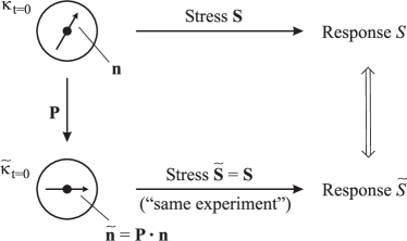
Figure 5: Anisotropy of the CAFFE flow law: If the same stress ($\tilde{\mathbf{S}}=\mathbf{S}$) is applied to two rotated initial configurations ($\kappa_{t=0}$, $\tilde{\kappa}_{t=0}$), the responses $S$ and $\tilde{S}$ are different in general.

4.2 Anisotropic behavior for simple shear

Let us illustrate the anisotropic behavior of the CAFFE flow law by a simple example. For the vertical single maximum fabric

$$\varrho^{\ast}(\mathbf{x},\mathbf{n},t)=\varrho(\mathbf{x},t)\,\delta(\mathbf{n}-\mathbf{e}_{3})$$ (40)

and the simple shear deformation

$$\mathbf{L}=\left(\begin{array}[]{ccc}0&0&\gamma\\ 0&0&0\\ 0&0&0\end{array}\right)\quad\Rightarrow\quad\mathbf{D}=\left(\begin{array}[]{ccc}0&0&\frac{\gamma}{2}\\ 0&0&0\\ \frac{\gamma}{2}&0&0\end{array}\right)\,,$$ (41)

we find

$$\frac{\varrho^{\ast}}{\varrho}=\delta(\mathbf{n}-\mathbf{e}_{3})\,,\quad\mathbf{S}=\left(\begin{array}[]{ccc}0&0&\tau\\ 0&0&0\\ \tau&0&0\end{array}\right)\,,\quad S^{\ast}(\mathbf{e}_{3})=\frac{5}{2}\quad\Rightarrow\quad S=\frac{5}{2}\,.$$ (42)

Thus, the $x$-$z$ component of the flow law (17) yields

$$\gamma=2A\hat{E}(\mbox{$\frac{5}{2}$})\,\tau^{n}=2AE_{\mathrm{max}}\tau^{n}\,,$$ (43)

where the explicit definition of the function $\hat{E}(S)$ [Eq. (27)] has been used.

Now we rotate the sample around the direction $\mathbf{e}_{2}$ by 45^∘ and keep the experimental apparatus fixed [apply the same stress in the sense of Eq. (37)]. In this case, the OMD changes as follows,

$$\varrho^{\ast}=\varrho\,\,\delta(\mathbf{n}-\mathbf{e}_{13}),\qquad\mathbf{e}_{13}=\left(\begin{array}[]{c}\frac{1}{\sqrt{2}}\\ 0\\ \frac{1}{\sqrt{2}}\end{array}\right)\,,$$ (44)

while the state of stress (42)₂ is unchanged. The species deformability is equal to zero for the orientation $\mathbf{e}_{13}$,

$$S^{\ast}(\mathbf{e}_{13})=0\quad\Rightarrow\quad S=0\,.$$ (45)

It follows that the stretching tensor evaluated with the flow law (17) yields the shear rate

$$\gamma=2A\hat{E}(0)\,\tau^{n}=2AE_{\mathrm{min}}\tau^{n}\,.$$ (46)

Since $E_{\mathrm{min}}\ll{}E_{\mathrm{max}}$, the shear rate of Eq. (46) is much smaller than that of Eq. (43). In other words, the material response of the ice specimen has changed considerably due to the $45^{\circ}$ rotation of its initial configuration. This fulfills clearly the criterion for an anisotropic material.

4.3 Isotropic, anisotropic, collinear and non-collinear flow laws

On the one hand, the classical Glen flow law

$$\mathbf{D}=A\,\left(\frac{\mathrm{tr}(\mathbf{S}^{2})}{2}\right)^{(n-1)/2}\,\mathbf{S}\,,$$ (47)

which results from the CAFFE flow law (17) by setting $\hat{E}(S)\equiv{}1$, is isotropic and collinear with respect to the tensors $\mathbf{D}$ and $\mathbf{S}$. On the other hand, many anisotropic flow laws published so far relate $\mathbf{D}$ and $\mathbf{S}$ by tensor quantities (Lliboutry 1993, Azuma 1994, Mangeney et al. 1996, Svendsen and Hutter 1996, Gödert and Hutter 1998, Thorsteinsson 2001, Morland and Staroszczyk 2003, Gillet-Chaulet et al. 2005), thus giving up the collinearity between $\mathbf{D}$ and $\mathbf{S}$.

This often leads to the misconception (at least in the glaciological community) that isotropic flow laws must be collinear and anisotropic flow laws must be non-collinear with respect to $\mathbf{D}$ and $\mathbf{S}$. However, this is not the case. As we have seen above, the CAFFE flow law is anisotropic, but collinear. Conversely, a non-collinear flow law is not necessarily anisotropic. An example is the general Reiner-Rivlin flow law for isotropic viscous fluids (e.g. Liu 2002, p. 109). For the incompressible case, it reads

$$\mathbf{S}=\alpha_{1}\mathbf{D}+\alpha_{2}\left(\mathbf{D}^{2}-\frac{\mathrm{tr}\,(\mathbf{D}^{2})}{3}\,\mathbf{I}\right)\,,$$ (48)

where $\alpha_{1}$ and $\alpha_{2}$ are material parameters. Provided that $\alpha_{2}\neq{}0$, this flow law is evidently non-collinear. So we highlight that isotropy/anisotropy and collinearity/non-collinearity are two entirely different concepts, and all four possible combinations can be realized.

The disadvantage of using a collinear anisotropic flow law is that, for a given fabric and a given state of stretching, we select a single viscosity of the polycrystal that is the same for every components of the stress deviator. However, in reality, for complex states of stretching (superposition of compression and shear etc.) different directions will show different degrees of softening or hardening. This shortcoming is a tribute to the simple formulation with a scalar enhancement factor, which allows to set up the flow law with only two well-known parameters ($E_{\mathrm{min}}$, $E_{\mathrm{max}}$).

5 Conclusion

We have presented a constitutive model for the dynamics of large polar ice masses. This CAFFE model consists of an anisotropic generalization of Glen’s flow law based on a scalar enhancement factor, and a fabric evolution equation based on an orientation mass balance. The latter arises from the framework of Mixtures with Continuous Diversity and uses the orientation mass density as the variable which describes the anisotropic fabric. Three constitutive quantities have been introduced, namely the orientation transition rate due to grain rotation, the orientation flux and the specific mass production rate. They have been linked to the physical processes of grain rotation, rotation recrystallization (polygonization) and grain boundary migration (migration recrystallization), respectively. The anisotropy of the CAFFE flow law has been proven, and in that context it has been emphasized that isotropy/anisotropy and collinearity/non-collinearity (between the stress and stretching tensors) must be clearly separated. Some applications of the CAFFE model to simple deformation states have been discussed (in the appendix), for which analytical solutions could be obtained, and which could easily be checked for their physical plausibility and consistency with observations.

Due to its relative simplicity, the CAFFE model is suitable for implementation in ice-flow models. This has already been done by Seddik et al. (2008) for a one-dimensional model of the site of the EPICA ice core at Kohnen Station in Dronning Maud Land, East Antarctica (EPICA Community Members 2006), and by Seddik (2008) and Seddik et al. (2009) for the three-dimensional, full-Stokes model Elmer/Ice in order to simulate the ice flow in the vicinity within 100 km around the Dome Fuji drill site (Motoyama 2007) in central East Antarctica.

Appendix A Examples for the evolution of the orientation mass density

A.1 Evolution due to grain rotation

The deck-of-cards deformation mechanism (grain rotation) implies that the $c$-axis of a crystallite in the polycrystalline aggregate rotates towards the axes of compression and away from that of extension. This is illustrated graphically in Fig. 2 for the case of rotated pure shear (simple shear) and described mathematically by Eq. (11), provided that the constitutive parameter $\iota$ is positive. Equation (11) fulfills the principle of material frame indifference. Thus, if the rules for compression and for extension are satisfied, then the rules for simple shear are a direct consequence. Here we give some simple examples in which this can explicitly be seen.

We use a Cartesian frame of reference for which the orientation $\mathbf{n}$ of the $c$-axis is parameterized by Eq. (4). For uniaxial vertical compression (transversely isotropic horizontal extension), the stretching tensor is

$$\mathbf{D}=\left(\begin{array}[]{ccc}\frac{\varepsilon}{2}&0&0\\ 0&\frac{\varepsilon}{2}&0\\ 0&0&-\varepsilon\end{array}\right)=\frac{1}{2}\,\varepsilon\,\mathbf{e}_{1}\,\mathbf{e}_{1}+\frac{1}{2}\,\varepsilon\,\mathbf{e}_{2}\,\mathbf{e}_{2}-\varepsilon\,\mathbf{e}_{3}\,\mathbf{e}_{3}\,,$$ (49)

where $\varepsilon>0$ holds. From Eqs. (4), (11) and (49) we derive the explicit form of the orientation transition rate due to grain rotation,

$$\mathbf{u}_{\mathrm{gr}}^{\ast} = -\frac{3}{4}\,\iota\,\varepsilon\sin 2\theta\left(\begin{array}[]{c}\cos\varphi\cos\theta\\ \sin\varphi\cos\theta\\ -\sin\theta\end{array}\right)$$ (53)

$$= -\frac{3}{4}\,\iota\,\varepsilon\sin 2\theta\,(\cos\varphi\cos\theta\,\mathbf{e}_{1}+\sin\varphi\cos\theta\,\mathbf{e}_{2}-\sin\theta\,\mathbf{e}_{3})\,.$$ (54)

The direction of $\mathbf{u}_{\mathrm{gr}}^{\ast}$ is coherent with the rules of Fig. 2a (see also Fig. 1b): The third component $\mathbf{u}_{\mathrm{gr}}^{\ast}\cdot\mathbf{e}_{3}$ is positive when $\theta<\pi/2$ and negative when $\theta>\pi/2$. If the crystallites are in the plane spanned by $\mathbf{e}_{1}$ and $\mathbf{e}_{3}$ ($\varphi=0$), Eq. (54) simplifies to

$$\varphi=0\quad\Rightarrow\quad\mathbf{u}_{\mathrm{gr}}^{\ast}=\frac{3}{4}\,\iota\,\varepsilon\sin 2\theta\left(\begin{array}[]{c}-\cos\theta\\ 0\\ \sin\theta\end{array}\right)\,,$$ (55)

and if they are in the plane spanned by $\mathbf{e}_{2}$ and $\mathbf{e}_{3}$ ($\varphi=\pi/2$), we find

$$\varphi=\frac{\pi}{2}\quad\Rightarrow\quad\mathbf{u}_{\mathrm{gr}}^{\ast}=\frac{3}{4}\,\iota\,\varepsilon\sin 2\theta\left(\begin{array}[]{c}0\\ -\cos\theta\\ \sin\theta\end{array}\right)\,.$$ (56)

It is worth noting that the norm of $\mathbf{u}_{\mathrm{gr}}^{\ast}$ which results from Eqs. (54), (55) or (56) shows the explicit dependence on the Schmidt factor $\sin{}2\theta$ that Azuma and Higashi (1985) recognized experimentally. The presence of the Schmidt factor guarantees that crystallites with vertical and horizontal orientations do not rotate, while those at orientations $45^{\circ}$ off the vertical show maximum rotation.

If the uniaxial compression is along the first ($\mathbf{e}_{1}$) instead of the third $(\mathbf{e}_{3})$ axis of the frame of reference, the orientation transition rate due to grain rotation takes the form

$$\mathbf{D}=\left(\begin{array}[]{ccc}-\varepsilon&0&0\\ 0&\frac{\varepsilon}{2}&0\\ 0&0&\frac{\varepsilon}{2}\end{array}\right)\quad\Rightarrow\quad\mathbf{u}_{\mathrm{gr}}^{\ast}=\iota\,\varepsilon\left(\begin{array}[]{c}\sin\theta\cos\varphi+B\left(\theta,\varphi\right)\sin\theta\cos\varphi\\ -\frac{1}{2}\sin\theta\sin\varphi+B\left(\theta,\varphi\right)\sin\theta\sin\varphi\\ -\frac{1}{2}\cos\theta+B\left(\theta,\varphi\right)\cos\theta\end{array}\right)\,,$$ (57)

where

$$B\left(\theta,\varphi\right)\equiv-\sin\theta\cos\varphi\sin\theta\cos\varphi+\frac{1}{2}\sin\theta\sin\varphi\sin\theta\sin\varphi+\frac{1}{2}\cos\theta\cos\theta\,.$$ (58)

The difference to Eq. (54) arises only because the spherical coordinate system, which underlies the representation of the unit vector $\mathbf{n}$ in Eq. (4), is more convenient for the vertical compression (49) than for the horizontal compression (57)₁.

For a planar elongation (or pure shear) state of deformation,

$$\mathbf{D}=\left(\begin{array}[]{ccc}\varepsilon&0&0\\ 0&0&0\\ 0&0&-\varepsilon\end{array}\right)=\varepsilon\,\,\mathbf{e}_{1}\,\mathbf{e}_{1}-\varepsilon\,\,\mathbf{e}_{3}\,\mathbf{e}_{3}\,,$$ (59)

the orientation transition rate due to grain rotation results from Eqs. (4), (11) and (59) as

$$\mathbf{u}_{\mathrm{gr}}^{\ast}=\iota\,\varepsilon\left(\begin{array}[]{c}(-1+\sin\theta\cos\varphi\sin\theta\cos\varphi-\cos\theta\cos\theta)\,\sin\theta\cos\varphi\\ 0\\ \sin\theta\sin\theta\,(1+\cos\varphi\cos\varphi)\,\cos\theta\end{array}\right)\,,$$ (60)

which, in the plane spanned by $\mathbf{e}_{1}$ and $\mathbf{e}_{3}$, is

$$\varphi=0\quad\Rightarrow\quad\mathbf{u}_{\mathrm{gr}}^{\ast}=\iota\,\varepsilon\sin 2\theta\left(\begin{array}[]{c}-\cos\theta\\ 0\\ \sin\theta\end{array}\right)\,.$$ (61)

This is larger by the factor $4/3$ compared to the orientation transition rate of Eq. (55)₂. The reason for this difference is that the component $D_{22}$ does not contribute to grain rotation in the plane spanned by $\mathbf{e}_{1}$ and $\mathbf{e}_{3}$, which makes the orientation transition rate in the case of Eq. (61) (where $D_{22}=0$) faster than in the case of Eq. (55) (where $D_{22}=\varepsilon/2$).

For the simple shear situation of Eq. (41), which is illustrated in Fig. 2b, we find for the orientation transition rate due to grain rotation

$$\mathbf{u}_{\mathrm{gr}}^{\ast}=\iota\,\frac{\gamma}{2}\left(\begin{array}[]{c}\cos\theta\,(2\sin^{2}\theta\cos^{2}\varphi-1)\\ \frac{1}{2}\sin\theta\sin 2\theta\sin 2\varphi\\ \sin\theta\cos\varphi\cos 2\theta\end{array}\right)\,,$$ (62)

which, in the plane spanned by $\mathbf{e}_{1}$ and $\mathbf{e}_{3}$, gives

$$\varphi=0\quad\Rightarrow\quad\mathbf{u}_{\mathrm{gr}}^{\ast}=\iota\,\frac{\gamma}{2}\cos 2\theta\left(\begin{array}[]{c}-\cos\theta\\ 0\\ \sin\theta\end{array}\right)\,.$$ (63)

The direction of $\mathbf{u}_{\mathrm{gr}}^{\ast}$ is once more consistent with the rules of Fig. 2b (see also Fig. 1b). For instance, for crystallites oriented upward within $\theta<\pi/4$ and a positive shear rate $\gamma>0$, the component of $\mathbf{u}_{\mathrm{gr}}^{\ast}$ along $\mathbf{e}_{1}$ is negative.

A.2 Evolution due to recrystallization

We now give some examples for the recrystallization term of Eq. (14) for standard deformation situations, and also provide a model of the experiments by Budd and Jacka (1989) for uniaxial compression with isotropic horizontal extension.

For the case of pure shear rate as defined in Eq. (59), crystallites oriented vertically have a vanishing species deformability,

$$\mathbf{n}=\mathbf{e}_{3}\quad\Rightarrow\quad D^{\ast}=5\,\frac{(\mathbf{D}\cdot\mathbf{n})^{2}-\left((\mathbf{D}\cdot\mathbf{n})\cdot\mathbf{n}\right)^{2}}{\mathrm{tr}(\mathbf{D}^{2})}=5\,\frac{\varepsilon^{2}-\varepsilon^{2}}{\frac{3}{2}\varepsilon^{2}}=0\,,$$ (64)

while crystallites inclined by $45^{\circ}$ off the vertical towards $\mathbf{e}_{1}$ have the maximum deformability,

$$\mathbf{n}=\mathbf{e}_{13}=\left(\begin{array}[]{c}\frac{1}{\sqrt{2}}\\ 0\\ \frac{1}{\sqrt{2}}\end{array}\right)\quad\Rightarrow\quad D^{\ast}=5\,\frac{(\mathbf{D}\cdot\mathbf{n})^{2}-\left((\mathbf{D}\cdot\mathbf{n})\cdot\mathbf{n}\right)^{2}}{\mathrm{tr}(\mathbf{D}^{2})}=5\,\frac{\varepsilon^{2}-0}{2\varepsilon^{2}}=\frac{5}{2}\,.$$ (65)

For general anisotropic fabrics, the averaged deformability $\langle{}D^{\ast}\rangle$ is between these extremes. It follows from Eq. (14) that the favourably oriented crystals with $\mathbf{n}=\mathbf{e}_{13}$ will grow ($\Gamma^{\ast}>0$) and the unfavourably oriented ones with $\mathbf{n}=\mathbf{e}_{3}$ will shrink ($\Gamma^{\ast}<0$). This is the physically expected behaviour.

The experiments by Budd and Jacka (1989) were carried out under the deformation regime of uniaxial compression with isotropic horizontal extension, as specified by Eq. (49). By using the parameterization (4) for general orientations $\mathbf{n}$, we compute the species deformability (15) as

$$D^{\ast}=\frac{15}{2}\sin^{2}\theta\cos^{2}\theta\,.$$ (66)

If at the initial time $t=0$, the OMD is random ($\varrho^{\ast}=\varrho/4\pi$, isotropic fabric), then

$$D=\langle D^{\ast}\rangle=\int_{\mathcal{S}^{2}}\frac{\varrho^{\ast}}{\varrho}\,D^{\ast}\,\mathrm{d}^{2}n=\int_{0}^{2\pi}\frac{1}{4\pi}\,\mathrm{d}\varphi\int_{0}^{\pi}\frac{15}{2}\,\sin^{2}\theta\cos^{2}\theta\,\sin\theta\,\mathrm{d}\theta=1\,,$$ (67)

where $\mathrm{d}^{2}{}n=\sin\theta\,\mathrm{d}\theta\,\mathrm{d}\varphi$ and usual integration rules have been used. The specific mass production rate which results from Eqs. (14) and (67) is

$$\Gamma^{\ast}(\theta)=\hat{\Gamma}\left(\frac{15}{2}\sin^{2}\theta\cos^{2}\theta-1\right)=\frac{15}{8}\,\hat{\Gamma}\,\sin^{2}2\theta-\hat{\Gamma}\,.$$ (68)

Consequently, crystallites with $\theta\in\left(\frac{1}{2}\arcsin\sqrt{\frac{8}{15}},\,\frac{\pi}{2}-\frac{1}{2}\arcsin\sqrt{\frac{8}{15}}\right)$ grow [$\Gamma^{\ast}(\theta)>0$], while the others shrink [$\Gamma^{\ast}(\theta)<0$], and an anisotropic fabric evolves. If we do not consider grain rotation and rotation recrystallization, then, asymptotically for $t\to\infty$, we will obtain

$$\varrho^{\ast}=\frac{\varrho}{2\pi\sin\theta_{0}}\,\delta(\theta-\theta_{0}),\quad\mbox{with}\;\,\theta_{0}=45^{\circ}\,,$$ (69)

where $\delta$ is the Dirac delta function. Equation (69) is the mathematical representation of a girdle fabric (see e.g. Placidi and Hutter 2006a) in which all the crystallites are inclined by $45^{\circ}$ with respect to the vertical. If grain rotation is superimposed, these crystallites will experience an additional rotation towards the compression axis $\mathbf{e}_{3}$ [in accordance with Eq. (63) or Fig. 2a], so that the small girdle fabric observed by Jacka and Budd (1989) is deduced.

Another interesting example is the rotated pure shear (simple shear) regime of Eq. (41) for general orientations $\mathbf{n}$ represented by Eq. (4). The crystal deformability is computed for this case as

$$D^{\ast}=\frac{5}{2}\left[\cos^{2}\varphi\sin^{2}\theta+\cos^{2}\theta\,(1-4\cos^{2}\varphi\sin^{2}\theta)\right]\,.$$ (70)

If at the initial time $t=0$, the OMD is random ($\varrho^{\ast}=\varrho/4\pi$, isotropic fabric), then, analogue to Eqs. (67) and (68), we find

$$D=1$$ (71)

and

$$\Gamma^{\ast}(\theta,\varphi)=\frac{5}{2}\,\hat{\Gamma}\left[\cos^{2}\varphi\sin^{2}\theta+\cos^{2}\theta\,(1-4\cos^{2}\varphi\sin^{2}\theta)\right]-\hat{\Gamma}\,.$$ (72)

For times $t>0$, an anisotropic fabric evolves, because crystallites oriented near $\mathbf{n}=\mathbf{e}_{1}$ ($\theta\approx\pi/2$ and $\varphi\approx{}0$) or $\mathbf{n}=\mathbf{e}_{3}$ ($\theta\approx{}0$) grow and the others shrink. Hence, without local rigid body rotation, grain rotation and rotation recrystallization, asymptotically for $t\to\infty$ we will obtain the two-maxima fabric

$$\varrho^{\ast}=\frac{1}{2}\delta\left(\mathbf{n}-\mathbf{e}_{1}\right)+\frac{1}{2}\delta\left(\mathbf{n}-\mathbf{e}_{3}\right)\,.$$ (73)

If grain rotation and rigid body rotation are superimposed, the fabric reported by Kamb (1972) results.

References

- Azuma (1994) Azuma, N. 1994. A flow law for anisotropic ice and its application to ice sheets. Earth Planet. Sci. Lett., 128 (3-4), 601–614.
- Azuma (1995) Azuma, N. 1995. A flow law for anisotropic polycrystalline ice under uniaxial compressive deformation. Cold Reg. Sci. Technol., 23 (2), 137–147.
- Azuma and Higashi (1985) Azuma, N. and A. Higashi. 1985. Formation processes of ice fabric patterns in ice sheets. Ann. Glaciol., 6, 130–134.
- Blenk et al. (1992) Blenk, S., H. Ehrentraut and W. Muschik. 1992. Macroscopic constitutive equations for liquid crystals induced by their mesoscopic orientation distribution. Int. J. Eng. Sci., 30, 1127–1143.
- Boehler (1987) Boehler, J. P. 1987. Applications of Tensor Functions in Solid Mechanics. Springer, New York.
- Budd and Jacka (1989) Budd, W. F. and T. H. Jacka. 1989. A review of ice rheology for ice sheet modelling. Cold Reg. Sci. Technol., 16 (2), 107–144.
- Dafalias (2001) Dafalias, Y. F. 2001. Orientation distribution function in non-affine rotations. J. Mech. Phys. Solids, 49, 2493–2516.
- Durand et al. (2008) Durand, G., A. Persson, D. Samyn and A. Svensson. 2008. Relation between neighbouring grains in the upper part of the NorthGRIP ice core – implications for rotation recrystallization. Earth Planet. Sci. Lett., 265 (3), 666–671. doi:10.1016/j.epsl.2007.11.002.
- EPICA Community Members (2006) EPICA Community Members. 2006. One-to-one coupling of glacial climate variability in Greenland and Antarctica. Nature, 444 (7116), 195–198. doi:10.1038/nature05301.
- Faria (2001) Faria, S. H. 2001. Mixtures with continuous diversity: general theory and application to polymer solutions. Cont. Mech. Thermodyn., 13, 91–120.
- Faria (2006a) Faria, S. H. 2006a. Creep and recrystallization of large polycrystalline masses. I. General continuum theory. Proc. R. Soc. A, 462 (2069), 1493–1514. doi:10.1098/rspa.2005.1610.
- Faria (2006b) Faria, S. H. 2006b. Creep and recrystallization of large polycrystalline masses. III. Continuum theory of ice sheets. Proc. R. Soc. A, 462 (2073), 2797–2816. doi:10.1098/rspa.2006.1698.
- Faria (2008) Faria, S. H. 2008. The symmetry group of the CAFFE model. J. Glaciol., 54 (187), 643–645.
- Faria et al. (2006) Faria, S. H., G. M. Kremer and K. Hutter. 2006. Creep and recrystallization of large polycrystalline masses. II. Constitutive theory for crystalline media with transversely isotropic grains. Proc. R. Soc. A, 462 (2070), 1699–1720. doi:10.1098/rspa.2005.1635.
- Gagliardini et al. (2009) Gagliardini, O., F. Gillet-Chaulet and M. Montagnat. 2009. A review of anisotropic polar ice models: from crystal to ice-sheet flow models. In: T. Hondoh (Ed.), Physics of Ice Core Records Vol. 2. Yoshioka Publishing, Kyoto, Japan. In press.
- Gillet-Chaulet et al. (2005) Gillet-Chaulet, F., O. Gagliardini, J. Meyssonnier, M. Montagnat and O. Castelnau. 2005. A user-friendly anisotropic flow law for ice-sheet modelling. J. Glaciol., 51 (172), 3–14.
- Glen (1955) Glen, J. W. 1955. The creep of polycrystalline ice. Proc. R. Soc. Lond. A, 228, 519–538.
- Gödert (2003) Gödert, G. 2003. A mesoscopic approach for modelling texture evolution of polar ice including recrystallization phenomena. Ann. Glaciol., 37, 23–28.
- Gödert and Hutter (1998) Gödert, G. and K. Hutter. 1998. Induced anisotropy in large ice shields: theory and its homogenization. Cont. Mech. Thermodyn., 10 (5), 293–318.
- Hutter (1983) Hutter, K. 1983. Theoretical Glaciology; Material Science of Ice and the Mechanics of Glaciers and Ice Sheets. D. Reidel Publishing Company, Dordrecht, The Netherlands.
- Jacka and Budd (1989) Jacka, T. H. and W. F. Budd. 1989. Isotropic and anisotropic flow relations for ice dynamics. Ann. Glaciol., 12, 81–84.
- Kamb (1972) Kamb, B. 1972. Experimental recrystallization of ice under stress. In: H. C. Heard, I. Y. Borg, N. L. Carter and C. B. Raileigh (Eds.), Flow and Fracture of Rocks, pp. 211–241. American Geophysical Union, Washington DC.
- Larson (1988) Larson, R. G. 1988. Constitutive equations for polymer melts and solutions. Butterworths series in chemical Engineering, Boston.
- Larson (1999) Larson, R. G. 1999. The structure and rheology of complex fluids. Oxford University press.
- Liu (2002) Liu, I.-S. 2002. Continuum Mechanics. Springer, Berlin etc.
- Lliboutry (1993) Lliboutry, L. 1993. Anisotropic, transversely isotropic nonlinear viscosity of rock ice and rheological parameters inferred from homogenization. Int. J. Plast., 9, 619–632.
- Mangeney et al. (1996) Mangeney, A., F. Califano and O. Castelnau. 1996. Isothermal flow of an anisotropic ice sheet in the vicinity of an ice divide. J. Geophys. Res., 101 (B12), 28189–28204.
- Massart et al. (2004) Massart, T. J., R. H. J. Peerlings and M. G. D. Geers. 2004. Mesoscopic modeling of failure and damage-induced anisotropy in brick masonry. European Journal of Mechanics - A/Solids, 23 (5), 719–735. doi:10.1016/j.euromechsol.2004.05.003.
- McConnel (1891) McConnel, J. C. 1891. On the plasticity of an ice crystal. Proc. R. Soc. Lond. A, 49, 323–343.
- Miyamoto (1999) Miyamoto, A. 1999. Mechanical properties and crystal textures of Greenland deep ice cores. Doctoral thesis, Hokkaido University, Sapporo, Japan.
- Morland and Staroszczyk (2003) Morland, L. W. and R. Staroszczyk. 2003. Stress and strain-rate formulations for fabric evolution in polar ice. Cont. Mech. Thermodyn., 15 (1), 55–71.
- Motoyama (2007) Motoyama, H. 2007. The second deep ice coring project at Dome Fuji, Antarctica. Sci. Drill., 5, 41–43. doi:10.2204/iodp.sd.5.05.2007.
- Müller (1985) Müller, I. 1985. Thermodynamics. Pitman Advanced Publishing Program, Boston.
- Nye (1952) Nye, J. F. 1952. The distribution of stress and velocity in glaciers and ice sheets. Proc. R. Soc. Lond. A, 239, 113–133.
- Papenfuss (2000) Papenfuss, C. 2000. Theory of liquid crystals as an example of mesoscopic continuum mechanics. Comput. Mater. Sci., 19, 45 52.
- Papenfuss and Van (2008) Papenfuss, C. and P. Van. 2008. Scalar, vectorial, and tensorial damage parameters from the mesoscopic background. Proceedings of the Estonian Academy of Sciences, 57 (3), 132–141.
- Paterson (1994) Paterson, W. S. B. 1994. The Physics of Glaciers. Pergamon Press, Oxford etc., 3rd ed.
- Pimienta et al. (1987) Pimienta, P., P. Duval and V. Y. Lipenkov. 1987. Mechanical behaviour of anisotropic polar ice. In: E. D. Waddington and J. S. Walder (Eds.), The Physical Basis of Ice Sheet Modelling, IAHS Publication No. 170, pp. 57–66. IAHS Press, Wallingford, UK.
- Placidi (2004) Placidi, L. 2004. Thermodynamically consistent formulation of induced anisotropy in polar ice accounting for grain-rotation, grain-size evolution and recrystallization. Doctoral thesis, Department of Mechanics, Darmstadt University of Technology, Germany. URL http://elib.tu-darmstadt.de/diss/000614/.
- Placidi (2005) Placidi, L. 2005. Microstructured continua treated by the theory of mixtures. Doctoral thesis, University of Rome “La Sapienza”, Italy.
- Placidi et al. (2004) Placidi, L., S. H. Faria and K. Hutter. 2004. On the role of grain growth, recrystallization and polygonization in a continuum theory for anisotropic ice sheets. Ann. Glaciol., 39, 49–52.
- Placidi and Hutter (2004) Placidi, L. and K. Hutter. 2004. Characteristics of orientation and grain-size distributions. In: Proceedings of the 21st International Congress of Theoretical and Applied Mechanics. Warsaw, Poland.