Component-Wise Markov Chain Monte Carlo: Uniform and Geometric Ergodicity under Mixing and Composition

Abstract

It is common practice in Markov chain Monte Carlo to update the simulation one variable (or sub-block of variables) at a time, rather than conduct a single full-dimensional update. When it is possible to draw from each full-conditional distribution associated with the target this is just a Gibbs sampler. Often at least one of the Gibbs updates is replaced with a Metropolis–Hastings step, yielding a Metropolis–Hastings-within-Gibbs algorithm. Strategies for combining component-wise updates include composition, random sequence and random scans. While these strategies can ease MCMC implementation and produce superior empirical performance compared to full-dimensional updates, the theoretical convergence properties of the associated Markov chains have received limited attention. We present conditions under which some component-wise Markov chains converge to the stationary distribution at a geometric rate. We pay particular attention to the connections between the convergence rates of the various component-wise strategies. This is important since it ensures the existence of tools that an MCMC practitioner can use to be as confident in the simulation results as if they were based on independent and identically distributed samples. We illustrate our results in two examples including a hierarchical linear mixed model and one involving maximum likelihood estimation for mixed models.

, and

1 Introduction

Let $\varpi$ be a probability distribution having support $\mathsf{X}\subseteq\mathbb{R}^{q}$, $q\geq 1$. The fundamental Markov chain Monte Carlo (MCMC) method for making draws from $\varpi$ is the Metropolis–Hastings algorithm, described here. Let $X^{(k)}=x$ denote the current state, and suppose $\varpi$ has a density function $\pi$. Let $p(\cdot,\cdot)$ denote the user-defined proposal density. The updated state $X^{(k+1)}$ is obtained via the following:

1. Simulate $x^{*}$ from proposal density $p(x,\cdot)$.

2. Calculate acceptance probability $\alpha(x,x^{*})$, where

   $$\alpha(x,y)=\min\biggl{\{}1,\frac{\pi(y)}{\pi(x)}\frac{p(y,x)}{p(x,y)}\biggr{\}}.$$

3. Set

   $$X^{(k+1)}=\cases{x^{*},&with probability $\alpha\bigl{(}x,x^{*}\bigr{)}$,\cr x,&with probability $1-\alpha\bigl{(}x,x^{*}\bigr{)}$.}$$

Thus, creating a Metropolis–Hastings sampler boils down to choosing a proposal density $p(\cdot,\cdot)$. If$p(x,y)=p(y,x)$, this is a Metropolis algorithm. If, further, $p(x,y)=p(x-y)=p(y-x)$ for all $x$ and $y$, it is a Metropolis random walk. When the proposal $p(\cdot)$ does not depend on the current state the chain is a Metropolis–Hastings independence sampler(MHIS).

The selection of the proposal density can be challenging, particularly in problems where $q$ is large or the support of $\varpi$ is complicated. This has led to investigation of optimal scaling of Metropolis algorithms and so-called adaptive algorithms which allow the proposal kernel to change over the course of the simulation (see, e.g., Bédard and Rosenthal (2008); Rosenthal (2011)). An alternative to full-dimensional updates is a component-wise approach where we update one variable (or sub-block of variables) at a time.

The choice between full-dimensional and component-wise updates is frequently unclear (see, e.g., Roberts and Sahu (1997)), although a general guideline seems to be that updating as a single block may not be advantageous if the components of $\varpi$ are only weakly correlated. For example, Neal and Roberts (2006) considered target distributions having independent and identically distributed components and showed that for an idealized version of a component-wise Metropolis algorithm it is optimal to update only one variable at a time. On the other hand, these authors also showed that when using Metropolis adjusted Langevin algorithms, block updating is more efficient.

Whatever MCMC method is used, an important consideration is the rate of convergence of the chain to its stationary distribution. Let $\mathcal{B}$ be the Borel $\sigma$-algebra on $\mathsf{X}$ and let $P^{n}(x,dy)$ denote the $n$-step Markov transition kernel, that is, for any $x\in\mathsf{X}$, $A\in\mathcal{B}$, and $n\in\mathbb{Z}^{+}$, $P^{n}(x,A)=\operatorname{Pr}(X^{(n+j)}\in A|X^{(j)}=x)$ for the Markov chain $\Phi=\{X^{(0)},X^{(1)},X^{(2)},\ldots\}$. Let $\|\cdot\|$ denote the total variation norm. If the chain is Harris ergodic, then for all $x\in\mathsf{X}$ we have $\|P^{n}(x,\cdot)-\varpi(\cdot)\|\to 0$ as $n\to\infty$. Now suppose there exist a real-valued function $M(x)$ on $\mathsf{X}$ and $0<t<1$ such that

$$\bigl{\|}P^{n}(x,\cdot)-\varpi(\cdot)\bigr{\|}\leq M(x)t^{n}.$$ (1)

If $M$ is bounded, then $\Phi$ is uniformly ergodic and otherwise it is geometrically ergodic.

A common goal of an MCMC experiment is to evaluate the quantity $E_{\varpi}g=\int_{\mathsf{X}}{g(x)\varpi(dx)}$, where $g$ is a real-valued function on $\mathsf{X}$ whose expectation exists. Upon simulation of the Markov chain, $E_{\varpi}g$ is approximated by the sample average $\bar{g}_{n}=\break n^{-1}\sum_{i=0}^{n-1}g(X^{(i)})$. This approximation is usually justified through Birkhoff’s ergodic theorem. Now, along with a moment condition on $g$, the existence of $M$ and $t$ in (1) ensures the existence of a central limit theorem for the Monte Carlo error, that is, there exists $0<\sigma^{2}_{g}<\infty$ such that, as $n\to\infty$,

$$\sqrt{n}(\bar{g}_{n}-E_{\varpi}g)\stackrel{{\scriptstyle d}}{{\to}}\mathrm{N}\bigl{(}0,\sigma_{g}^{2}\bigr{)}.$$ (2)

Along with various moment conditions, the existence of $M$ and $t$ in (1) is also a key sufficient condition for using a variety of methods such as batch means, spectral methods or regenerative simulation to construct a strongly consistent estimator of $\sigma_{g}^{2}$, ensuring asymptotically valid Monte Carlo standard errors (Atchadé (2011); Flegal and Jones (2010); Hobert et al. (2002); Jones et al. (2006)). Thus, when $\Phi$ is at least geometrically ergodic, a practitioner has the tools to be as confident in their simulations as if it were possible to make independent and identically distributed draws from $\varpi$ (Flegal, Haran and Jones (2008); Flegal and Jones (2011)).

Much work has been done on establishing geometric and uniform ergodicity of various versions of Metropolis–Hastings when full-dimensional updates are used; for example, Mengersen and Tweedie (1996) and Tierney (1994) studied the MHIS while Johnson and Geyer (2012), Mengersen and Tweedie (1996), Roberts and Tweedie (1996), Jarner andHansen (2000), Christensen, Møller and Waagepetersen (2001) have established conditions under which Metropolis yields a geometrically ergodic chain. Other research on establishing convergence rates of Metropolis–Hastings chains includes Geyer (1999), Jarner and Hansen (2000) and Meyn and Tweedie (1994). Note well that none of these convergence rate results apply to component-wise implementations of Metropolis–Hastings. Also, a full-dimensional updating algorithm may fail to be geometrically ergodic while many component-wise updating samplers are. Consider the following simple example.

Example 1.

Suppose $\log\pi(x,y)=-(x^{2}+x^{2}y^{2}+y^{2})$. Roberts and Tweedie (1996) showed that a Metropolis random walk having target $\pi$ cannot be geometrically ergodic. Thus, one might consider component-wise methods where the target of each update is the relevant conditional distribution, $X|Y=y\sim\mathrm{N}(0,\frac{1}{2}(1+y^{2})^{-1})$ or $Y|X=x\sim\mathrm{N}(0,\frac{1}{2}(1+x^{2})^{-1})$. Fort et al. (2003) established geometric ergodicity of the uniform random scan Metropolis random walk. That is, at each step one of the components is selected with probability $1/2$ to remain fixed while a Metropolis random walk step is performed for the other. We will show that the Gibbs sampler is geometrically ergodic as are the random scan Gibbs and random sequence Gibbs samplers for any selection probabilities.

We study conditions for ensuring geometric or uniform ergodicity for several component-wise strategies. Despite the near ubiquity of component-wise methods in MCMC practice, there has been very little work on this problem. In particular, there has been almost none in the case where the component-wise updates are done with Metropolis–Hastings (but see Fort et al. (2003); Jones, Roberts and Rosenthal (2013); Roberts and Rosenthal (1998)). The one component-wise method that has received some attention in the literature is the Gibbs sampler, especially the two-variable deterministically updated Gibbs sampler; see, for example, the work in Doss and Hobert (2010), Hobert and Geyer (1998), Hobert et al. (2002), Johnson and Jones (2010), Jones and Hobert (2004), Marchev and Hobert (2004),Papaspiliopoulos and Roberts (2008), Roberts and Polson (1994), Roberts and Rosenthal (1999), Román and Hobert (2012), Rosenthal (1995, 1996), Roy and Hobert (2007), Tan and Hobert (2009) and Tierney (1994).

In Section 2 we fix some notation, state assumptions and develop a general framework for component-wise updates. Then in Section 3 we study the convergence rates of component-wise methods. In particular, we connect the convergence rate of deterministic scan samplers with random sequence scan and random scan methods. We also develop conditions for the uniform ergodicity of component-wise versions of the Metropolis–Hastings algorithm with state-independent candidate distributions. Along the way we apply our results to two practically relevant examples, including the Gibbs sampler for a Bayesian linear mixed model and one involving maximum likelihood estimation for mixed models, and provide empirical comparisons between samplers using component-wise updates and their full-dimensional counterparts. Notably, the empirical performance of the component-wise samplers is compellingly better, thus providing further support for the use of component-wise methods in practical problems; see also Caffo, Jank and Jones (2005), Coull et al. (2001), Johnson and Jones (2010), Jones et al. (2006), Jones and Hobert (2001), Lee et al. (2013), McCulloch (1997) and Neath (2013). Proofs of our results and other technical material are given in the supplement to the current article (Johnson, Jones and Neath (2013)).

2 Component-Wise Updates

Two fundamental strategies for combining Markov kernels are mixing and composition. Suppose $P_{1},\ldots,\break P_{d}$ are Markov kernels having common invariant distribution $\varpi$. The general composition kernel is given by $P_{\mathrm{comp}}(x,\cdot)=(P_{1}\cdots P_{d})(x,\cdot)$. Let $\mathbb{P}^{d}=\{(r_{1},\ldots,\break r_{d})\in\mathbb{R}^{d}\mbox{: each }r_{i}>0,\sum_{i=1}^{d}r_{i}=1\}$. Define the general mixing kernel

$$P_{\mathrm{mix}}(x,\cdot)=r_{1}P_{1}(x,\cdot)+\cdots+r_{d}P_{d}(x,\cdot),\quad r\in\mathbb{P}^{d}.$$

Then $P_{\mathrm{mix}}$ and $P_{\mathrm{comp}}$ are Markov kernels preserving the invariance of $\varpi$ and we say that $P_{\mathrm{mix}}$ has selection probabilities $r$.

We can use these two strategies to create many component-wise algorithms. Suppose $\pi$ is a density of $\varpi$ with respect to a measure $\mu=\mu_{1}\times\cdots\times\mu_{d}$ and has support $\mathsf{X}=\mathsf{X}_{1}\times\cdots\times\mathsf{X}_{d}$ with Borel $\sigma$-algebra $\mathcal{B}$. We allow each $\mathsf{X}_{i}\subseteq\mathbb{R}^{b_{i}}$ so that the total dimension is $b_{1}+\cdots+b_{d}$. If $x\in\mathsf{X}$, set $x_{(i)}=x\setminus x_{i}$. For $i=1,\ldots,d$ let $g_{i}(y_{i}|x)$ be a density satisfying

$$\pi(y_{i}|x_{(i)})=\int g_{i}(y_{i}|x)\pi(x_{i}|x_{(i)})\mu_{i}(dx_{i}).$$ (3)

That is, the conditional density $\pi(x_{i}|x_{(i)})$ is invariant for $g_{i}(y_{i}|x)$. Note that (3) is trivially satisfied if $g_{i}$ corresponds to an elementary Gibbs update, that is, $g_{i}(y_{i}|x)=\pi(y_{i}|x_{(i)})$. Also, condition (3) is satisfied by construction if $g_{i}$ corresponds to a Metropolis–Hastings algorithm having $\pi(y_{i}|x_{(i)})$ as its target.

Given (3), define a Markov kernel $P_{i}$ as

$$P_{i}(x,A)=\int_{A}g_{i}(y_{i}|x)\delta(y_{(i)}-x_{(i)})\mu(dy)$$ (5)

$$\eqntext{\mbox{for }A\in\mathcal{B},}$$

where $\delta$ is Dirac’s delta. Then $\varpi$ is invariant for each $P_{i}$ so that $\varpi P_{i}=\varpi$ since

$$\int_{\mathsf{X}}\pi(x)g_{i}(y_{i}|x)\delta(y_{(i)}-x_{(i)})\mu(dx)=\pi(y).$$

Since component-wise updates are not $\varpi$-irreducible, we need to combine the $P_{i}$ in order to achieve a useful algorithm. Let $r\in\mathbb{P}^{d}$ be the selection probabilities corresponding to the components. Then we can write the random scan Markov kernel as

$$P_{\mathrm{RS}}(x,A)=\sum_{i=1}^{d}r_{i}P_{i}(x,A)$$ (6)

and it is obvious that $\varpi P_{\mathrm{RS}}=\varpi$. Moreover, $P_{\mathrm{RS}}$ admits a Markov transition density (Mtd)

$$h_{\mathrm{RS}}(y|x)=\sum_{i=1}^{d}r_{i}g_{i}(y_{i}|x)\delta(y_{(i)}-x_{(i)}).$$

Another way to combine the $P_{i}$ is through composition, that is, deterministically cycling through the component-wise updates one at a time, in which case the Markov kernel is

$$P_{C}(x,A)=(P_{1}\cdots P_{d})(x,A)$$ (7)

and it is easy to see that $\varpi P_{C}=\varpi$ and that the associated Mtd is

$$h_{C}(y|x)=g_{1}(y_{1}|x)g_{2}(y_{2}|y_{1},x_{(1)})\cdots g_{d}(y_{d}|y_{(d)},x_{d}).$$

There are $d!$ orders in which composition can be used and it is natural to consider using mixing to combine some of them. If $r\in\mathbb{P}^{p}$ for $p\leq d!$, the sequence mixing kernel is given by

$$P_{\mathrm{RQ}}(x,A)=\sum_{j=1}^{p}r_{j}P_{C,j}(x,A),$$ (8)

where the $P_{C,j}$ are kernels created via composition but in different orders. Since $\varpi P_{C,j}=\varpi$ for each $j$, it is easy to see that $\varpi P_{\mathrm{RQ}}=\varpi$. Clearly, the Mtd is

$$h_{\mathrm{RQ}}(y|x)=\sum_{j=1}^{p}r_{j}h_{C,j}(y|x).$$

Note that the kernels defined in (6), (7) and (8) are special cases of the general definitions of $P_{\mathrm{mix}}$ and $P_{\mathrm{comp}}$. We will employ the notation $P_{C}$, $P_{\mathrm{RS}}$ and $P_{\mathrm{RQ}}$ for the special case of component-wise updates, that is, when the $P_{i}$ satisfy (5).

3 Convergence Rates Under Component-Wise Updates

Most of the research on convergence rates of component-wise MCMC algorithms has focused on those formed by composition, such as deterministic scan Gibbs samplers. One of our goals in this section is to show that the convergence rates of samplers formed by mixing and composition are related in concrete ways. However, we begin with a brief description of some techniques for establishing the existence of $M$ and $t$ in (1); see Meyn and Tweedie [(1993), Chapter 15] and Roberts and Rosenthal (2004) for details and Jones and Hobert (2001) for an accessible introduction.

Recall that $\mathcal{B}$ is the Borel $\sigma$-algebra on $\mathsf{X}$ and $P^{n}(x,dy)$ denotes a $n$-step Markov transition kernel, that is, for any $x\in\mathsf{X}$, $A\in\mathcal{B}$, and $n\in\mathbb{Z}^{+}$, $P^{n}(x,A)=\operatorname{Pr}(X^{(n+j)}\in A|X^{(j)}=x)$ for the Markov chain $\Phi=\{X^{(0)},X^{(1)},X^{(2)},\ldots\}$.

Suppose there exist a positive integer $n_{0}$, an $\epsilon>0$, a set $C\in\mathcal{B}$, and a probability measure $Q$ on $\mathcal{B}$ such that

$$P^{n_{0}}(x,A)\geq\epsilon Q(A)\quad\mbox{for all }x\in C,A\in\mathcal{B}.$$ (9)

Then a minorization condition holds on the set $C$, called a small set. Uniform ergodicity is equivalent to the existence of a minorization condition on $\mathsf{X}$.

Let

$$\mathit{PV}(x):=E\bigl{[}V\bigl{(}X^{(t+1)}\bigr{)}|X^{(t)}=x\bigr{]}.$$ (10)

A drift condition holds if there exists some function $V\dvtx\mathsf{X}\to[1,\infty)$, constants $0<\gamma<1$ and $k<\infty$ and a set $C$ such that

$$\quad\mathit{PV}(x)\leq\gamma V(x)+kI_{C}(x)\quad\mbox{for all }x\in\mathsf{X}.$$ (11)

If $C$ is small, then (11) is equivalent to geometric ergodicity (Meyn and Tweedie (1993); Roberts and Rosenthal, 1997, 2004).

3.1 Uniform Ergodicity Under Mixing and Composition

We begin with some results concerning samplers $P_{\mathrm{mix}}$ and $P_{\mathrm{comp}}$, after which we will specialize to some component-wise samplers.

Theorem 1

If $P_{\mathrm{mix}}$ is uniformly ergodic for some selection probabilities, then it is uniformly ergodic for all selection probabilities.

It is easy to see that if one of the component samplers is uniformly ergodic, then $P_{\mathrm{mix}}$ will be uniformly ergodic. Also, it is sufficient to study $P_{\mathrm{comp}}$ to establish uniform ergodicity of $P_{\mathrm{mix}}$.

Theorem 2

Suppose $P_{\mathrm{comp}}$ is uniformly ergodic. Then the corresponding $P_{\mathrm{mix}}$ is uniformly ergodic for any selection probabilities.

For component-wise updates it can be difficult to establish uniform ergodicity of $P_{\mathrm{mix}}$ due to the form of its Mtd. Our next result follows directly from Theorems 1 and 2 and the observation that $P_{\mathrm{RS}}$ and $P_{\mathrm{RQ}}$ are special cases of $P_{\mathrm{mix}}$ and $P_{C}$ is a special case of $P_{\mathrm{comp}}$. See Łatuszynski, Roberts and Rosenthal (2013) and Roberts and Rosenthal (1997) for related results.

Theorem 3

If $P_{C}$ is uniformly ergodic, then $P_{\mathrm{RS}}$ and $P_{\mathrm{RQ}}$ are uniformly ergodic for any selection probabilities.

3.1.1 Component-wise independence samplers

It is clear that many component-wise Markov chains will not be uniformly ergodic. For example, it is well known that Metropolis random walks on $\mathbb{R}$ are not uniformly ergodic (Mengersen and Tweedie (1996)). Hence, when using such chains as the building blocks of a component-wise algorithm one does not expect to produce a uniformly ergodic Markov chain. On the other hand, Mengersen and Tweedie (1996) did show that the full-dimensional Metropolis–Hastings independence sampler can be uniformly ergodic. We now turn our attention to the component-wise algorithm where each component-wise update is a Metropolis–Hastings algorithm with state-independent proposals. In this case, the composition sampler, $P_{\mathrm{CIS}}$, the random sequence sampler, $P_{\mathrm{RQIS}}$, and the random scan sampler, $P_{\mathrm{RSIS}}$, are all component-wise independence samplers (CWIS).

We are interested in establishing conditions under which the CWIS are uniformly ergodic. By Theorem 3 it is sufficient to consider CIS. Note that since a typical $P_{\mathrm{CIS}}$ update will be some combination of accepted and rejected component-wise proposals, the $P_{\mathrm{CIS}}$ is not truly an independence sampler at all and, thus, the results of Mengersen and Tweedie (1996) are not applicable. It is, however, tempting to think that extending Mengersen and Tweedie’s (1996) work on MHIS to $P_{\mathrm{CIS}}$ will be straightforward. Let $p_{i}(\cdot)$, a density on $\mathsf{X}_{i}$, denote the state-independent proposal density for the $i$th update, $i=1,\ldots,d$. If we let $p(x)=\prod_{i=1}^{d}p_{i}(x_{i})$, a density on $\mathsf{X}$, is the existence of $\epsilon>0$ such that $p(x)\geq\epsilon\pi(x)$ a sufficient condition for uniform ergodicity of $P_{\mathrm{CIS}}$? If we attempt to directly generalize Mengersen and Tweedie’s (1996) argument, we are faced with $2^{d}$ cases to consider and, hence, this approach is fruitless. However, with a different approach we are able to give a pair of conditions that together are sufficient for uniform ergodicity of the CWIS.

To describe our results, we require a new notation. We will continue to let a subscript indicate the position of a vector component and a parenthetical superscript indicate the step in a Markov chain. Additionally, for each $i=1,\ldots,d$, let $x_{[i]}=(x_{1},\ldots,x_{i})$ and $x^{[i]}=(x_{i},\ldots,x_{d})$; let $x_{[0]}$ and $x^{[d+1]}$ be null (vectors of dimension 0). We can now state the result for CWIS.

Theorem 4

Consider the kernel $P_{\mathrm{CIS}}$ with proposal densities $p_{i}$ for $i=1,\ldots,d$. Define $p(x):=\prod_{i=1}^{d}p_{i}(x_{i})$, a density on $\mathsf{X}$. Further suppose there exists $\delta>0$ such that $p(x)\geq\delta\pi(x)$ for all $x\in\mathsf{X}$, and $\varepsilon>0$ such that for any $x,y\in\mathsf{X}$ with $\pi(x)>0$ and $\pi(y)>0$,

$$\qquad\pi(x)\pi(y) = \pi\bigl{(}x_{[i]},x^{[i+1]}\bigr{)}\pi\bigl{(}y_{[i]},y^{[i+1]}\bigr{)}$$

$$\geq \varepsilon\pi\bigl{(}x_{[i]},y^{[i+1]}\bigr{)}\pi\bigl{(}y_{[i]},x^{[i+1]}\bigr{)}>0$$

for each $i=1,\ldots,d-1$. Then, for any $x\in\mathsf{X}$ and $A\in\mathcal{B}(\mathsf{X})$,

$$P_{\mathrm{CIS}}(x,A)\geq\delta\varepsilon^{\lfloor d/2\rfloor}\pi(A)$$

and, thus, $P_{\mathrm{CIS}}$ is uniformly ergodic. Hence, $P_{\mathrm{RQIS}}$ and $P_{\mathrm{RSIS}}$ are also uniformly ergodic for any selection probabilities.

The following two corollaries indicate settings where the conditions of the theorem are easily verified.

Corollary 1

Consider the kernel $P_{\mathrm{CIS}}$ with proposal densities $p_{i}$ for $i=1,\ldots,d$. Define $p(x):=\prod_{i=1}^{d}p_{i}(x_{i})$, a density on $\mathsf{X}$. Further suppose there exists $\delta>0$ such that $p(x)\geq\delta\pi(x)$ for all $x\in\mathsf{X}$, and pairs of positive functions $g_{i}$ and $h_{i}$ on $\mathsf{X}_{i}$ for $i=1,\ldots,d$ such that

$$\prod_{i=1}^{d}g_{i}(x_{i})\leq\pi(x)\leq\prod_{i=1}^{d}h_{i}(x_{i})$$ (13)

for any $x\in\mathsf{X}$, and $\inf_{x_{i}\in\mathsf{X}_{i}}\{g_{i}(x_{i})/h_{i}(x_{i})\}>0$ for each $i=1,\ldots,d$. Then $P_{\mathrm{CIS}}$, $P_{\mathrm{RQIS}}$ and $P_{\mathrm{RSIS}}$ are all uniformly ergodic.

The conditions of Corollary 1 amount to requiring at most a weak form of dependence in the target distribution. The most obvious special case is when the components of $\pi$ are jointly independent, in which case (13) holds with equality on both sides.

Corollary 2

Consider the kernel $P_{\mathrm{CIS}}$ with proposal densities $p_{i}$ for $i=1,\ldots,d$. Define $p(x):=\prod_{i=1}^{d}p_{i}(x_{i})$, a density on $\mathsf{X}$. If there exist $0<a\leq b<\infty$ and $c>0$ such that $a\leq\pi(x)\leq b$ and $p(x)\geq c$ for $\varpi$-almost all $x$, then $P_{\mathrm{CIS}}$, $P_{\mathrm{RQIS}}$ and $P_{\mathrm{RSIS}}$ are all uniformly ergodic.

3.1.2 Maximum likelihood for mixed models

Let $Y_{i}=\{Y_{i1},\ldots,Y_{im_{i}}\}$ denote a vector of observable data, and let $U_{i}$ denote the unobservable $i$th random effect, for $i=1,\ldots,k$; let $U=(U_{1},\ldots,U_{k})$. Assume the $Y_{i}$ are independent with distribution specified conditionally on $U=u$, so that the joint density of $Y=\{Y_{ij}\dvtx j=1,\ldots,m_{i};i=1,\ldots,k\}$ is

$$f(y|u;\theta_{1})=\prod_{i=1}^{k}\prod_{j=1}^{m_{i}}f(y_{ij}|u_{i};\theta_{1}),$$

where $\theta_{1}$ denotes a vector of parameters. The $U_{i}$ are assumed to be independent, typically but not necessarily normally distributed, so the joint density of $U$ is $h(u;\theta_{2})=\prod_{i=1}^{k}h(u_{i};\theta_{2})$. Then the likelihood,

$$L(\theta;y)=\int f(y|u;\theta_{1})h(u;\theta_{2})\,du$$

is often analytically intractable so that calculating maximum likelihood estimates and their standard errors can be challenging. However, there are several Monte Carlo-based algorithms, such as Monte Carlo Newton–Raphson, Monte Carlo maximum likelihood and Monte Carlo EM, which are useful for finding maximum likelihood estimators of the unknown parameter $\theta=(\theta_{1},\theta_{2})$ (Caffo, Jank and Jones (2005); Hobert (2000); McCulloch (1997)). A common feature is that all three algorithms require simulation from the same target distribution, namely, the conditional distribution of the random effects given the data, that is, for a given value of $\theta$

$$h(u|y;\theta)\propto f(y|u;\theta_{1})h(u;\theta_{2}).$$

We consider four Markov chains having $h(u|y;\theta)$ as the invariant density; the three component-wise independence samplers, CIS, RQIS and RSIS having proposal densities $h(u_{i};\theta_{2})$ for $i=1,\ldots,k$ and a full-dimensional Metropolis–Hastings Independence Sampler (MHIS) with proposals drawn from themarginal distribution $h(u;\theta_{2})$. To this end, the following result holds.

Theorem 5

If there exists $B(y,\theta_{1})<\infty$ such that $f(y|u;\theta_{1})\leq B(y,\theta_{1})$ for all $u$, then the four Markov chains described above, MHIS, CIS, RQIS and RSIS having $h(u|y,\theta)$ as the invariant density, are uniformly ergodic.

We compare the empirical performance of theCWIS, the MHIS and a geometrically ergodic full-dimensional Metropolis random walk sampler in a concrete example in Section 4.2.

3.2 Geometric Ergodicity Under Mixing and Composition

Consider $P_{\mathrm{mix}}$ and suppose each of the kernels $P_{i}$ are geometrically ergodic in that there are nonnegative functions $M_{i}$ and $t_{i}\in(0,1)$ such that

$$\bigl{\|}P_{i}(x,\cdot)-\varpi(\cdot)\bigr{\|}\leq M_{i}(x)t_{i}^{n}.$$

Then the triangle inequality implies

$$\bigl{\|}P_{\mathrm{mix}}(x,\cdot)-\varpi(\cdot)\bigr{\|}$$

$$\quad\leq\bigl{[}r_{1}M_{1}(x)+\cdots+r_{d}M_{d}(x)\bigr{]}\bigl{[}\max\{t_{1},\ldots,t_{d}\}\bigr{]}^{n}$$

and, hence, we have the following observation: if each $P_{i}$ is geometrically ergodic, then so is $P_{\mathrm{mix}}$. This demonstrates one difference between establishing geometric and uniform ergodicity; recall that we only required one of the $P_{i}$ to be uniformly ergodic for $P_{\mathrm{mix}}$ to be uniformly ergodic. Also, this immediately implies that $P_{\mathrm{RQ}}$ is geometrically ergodic if each of the composition samplers are. However, it does not apply to $P_{\mathrm{RS}}$ since, in this case, each of the $P_{i}$ typically are not even $\varpi$-irreducible. On the other hand, we have an analogue of Theorem 1, albeit with an additional assumption. Recall that a Markov kernel $P$ is reversible with respect to $\varpi$ if

$$P(x,dy)\varpi(dx)=P(y,dx)\varpi(dy).$$

Theorem 6

Suppose $P_{\mathrm{mix}}$ is reversible with respect to $\varpi$ for all selection probabilities $r\in\mathbb{P}^{d}$. If $P_{\mathrm{mix}}$ is geometrically ergodic for some selection probability, then it is geometrically ergodic for all selection probabilities.

Note that a special case of Theorem 6 is that if $P_{\mathrm{RS}}$ is geometrically ergodic for some selection probability, then it is geometrically ergodic for all selection probabilities; see Jones, Roberts and Rosenthal (2013) for related results. Also, Theorem 6 does not apply to random sequence scan samplers since these are not reversible for all selection probabilities.

3.2.1 Two-variable settings

We consider the case where $\varpi$ has a density $\pi(x,y)$ with respect to $\mu_{1}\times\mu_{2}$ and has support $\mathsf{X}_{1}\times\mathsf{X}_{2}\subseteq\mathbb{R}^{b_{1}}\times\mathbb{R}^{b_{2}}$. Let $\pi_{X|Y}(x|y)$ and $\pi_{Y|X}(y|x)$ be the full conditional densities and $\pi_{X}$ and $\pi_{Y}$ be the marginal densities derived from $\pi$ ($\varpi_{X}$ and $\varpi_{Y}$ are the marginal distributions). This setting, though less general than that of the previous section, has many practical applications. For instance, it is the foundation for data augmentation methods (Hobert (2011); Tanner and Wong (1987)) and many MCMC methods for practically relevant statistical models (Johnson and Jones (2010); Román and Hobert (2012); Roy and Hobert (2007)). We will consider two settings here: specifically, we begin with the case where sampling from $\pi_{X|Y}$ and $\pi_{Y|X}$ is possible and later turn our attention to the case where one of the Gibbs updates is replaced by a Metropolis–Hastings update.

When sampling from $\pi_{X|Y}$ and $\pi_{Y|X}$ is easy the Markov kernel formed by composition, say, $P_{\mathrm{GS}}$, is the usual Gibbs sampler (GS) having Mtd

$$h_{\mathrm{GS}}\bigl{(}x^{\prime},y^{\prime}|x,y\bigr{)}=\pi_{X|Y}\bigl{(}x^{\prime}|y\bigr{)}\pi_{Y|X}\bigl{(}y^{\prime}|x^{\prime}\bigr{)}.$$ (14)

Of course, the other update order is also a Gibbs sampler, denoted $\tilde{P}_{\mathrm{GS}}$. Also, each of the marginal sequences $\{X^{(n)}\}$ and $\{Y^{(n)}\}$ have one-step Markov kernels $P_{X}$ and $P_{Y}$ with Mtds

$$h_{X}\bigl{(}x^{\prime}|x\bigr{)}=\int\pi_{X|Y}\bigl{(}x^{\prime}|y\bigr{)}\pi_{Y|X}(y|x)\mu_{2}(dy)$$

and

$$\quad h_{Y}\bigl{(}y^{\prime}|y\bigr{)}=\int\pi_{Y|X}\bigl{(}y^{\prime}|x\bigr{)}\pi_{X|Y}(x|y)\mu_{1}(dx),$$ (15)

respectively. Moreover, it is easy to see that $P_{Y}^{m}$ admits an $m$-step Mtd $h_{Y}^{m}(y^{\prime}|y)$ as do $P_{X}^{m}$, $P_{\mathrm{GS}}^{m}$ and $\tilde{P}_{\mathrm{GS}}^{m}$. Note that $\pi_{X}$ is invariant for $\{X^{(n)}\}$ and $\pi_{Y}$ is invariant for $\{Y^{(n)}\}$.

It is well known that $P_{X}$, $P_{Y}$, $P_{\mathrm{GS}}$ and $\tilde{P}_{\mathrm{GS}}$ all converge at the same qualitative rate (Diaconis, Khare and Saloff-Coste (2008); Robert (1995); Roberts and Rosenthal (2001)). In particular, if one is geometrically ergodic, then so are the others. This relationship has been routinely exploited in the analysis of Gibbs samplers for practically relevant statistical models, where it is often easier to analyze $P_{Y}$ or $P_{X}$ than $P_{\mathrm{GS}}$. Putting these observations together with our above work says that if one of $P_{X}$, $P_{Y}$, $P_{\mathrm{GS}}$ or $\tilde{P}_{\mathrm{GS}}$ are geometrically ergodic, then so are the others and so is the random sequence Gibbs sampler $P_{\mathrm{RQGS}}$.

The first result of this subsection connects the convergence rate of $P_{X}$, $P_{Y}$, $P_{\mathrm{GS}}$ and $\tilde{P}_{\mathrm{GS}}$ to the random scan Gibbs sampler $P_{\mathrm{RSGS}}$. Note that by using (10) and (15) we have that

$$P_{Y}W(y)=\int_{\mathsf{X}_{2}}W\bigl{(}y^{\prime}\bigr{)}h_{Y}\bigl{(}y^{\prime}|y\bigr{)}\mu_{2}\bigl{(}dy^{\prime}\bigr{)}.$$

Theorem 7

Suppose there exists $\lambda<1$, $W\dvtx\break\mathsf{X}_{2}\rightarrow\mathbb{R}^{+}$, $b<\infty$ such that

$$P_{Y}W(y)\leq\lambda W(y)+b.$$ (16)

Let $C_{d}=\{y\dvtx W(y)\leq d\}$ and suppose there is a $g\dvtx\break\mathsf{X}_{2}\to\mathbb{R}^{+}$ and a $d_{0}>0$ such that for some $m\geq 1$

$$\qquad h_{Y}^{m}\bigl{(}y^{\prime}|y\bigr{)}\geq g\bigl{(}y^{\prime}\bigr{)}\quad\mbox{for all }y\in C_{d}\mbox{ and }d\geq d_{0}.$$ (17)

Then $P_{Y}$, $P_{X}$, $P_{\mathrm{GS}}$ and $\tilde{P}_{\mathrm{GS}}$ are geometrically ergodic as are $P_{\mathrm{RQGS}}$ and $P_{\mathrm{RSGS}}$.

There is a simple sufficient condition for (17); suppose there is a $l\dvtx\mathsf{X}_{2}\to\mathbb{R}^{+}$ such that $\pi_{X|Y}(x|y)\geq l(x)$ for all $(x,y)\in\mathsf{X}_{1}\times C_{d}$ with $d\geq d_{0}$. Then if $y\in C_{d}$,

$$h_{Y}\bigl{(}y^{\prime}|y\bigr{)} = \int_{\mathsf{X}_{1}}\pi_{Y|X}\bigl{(}y^{\prime}|z\bigr{)}\pi_{X|Y}(z|y)\mu_{1}(dz)$$

$$\geq \int_{\mathsf{X}_{1}}\pi_{Y|X}\bigl{(}y^{\prime}|z\bigr{)}l(z)\mu_{1}(dz)=g\bigl{(}y^{\prime}\bigr{)}.$$

Although we do not state it formally, it is clear from our proof that the same conclusions obtain if we were to reformulate the conditions in terms of $P_{X}$ instead of $P_{Y}$.

Example 2.

Consider the Gibbs sampler defined in Example 1. If $W(y)=y^{2}$, it is easy to see that $P_{Y}W(y)\leq\lambda W(y)+0.5$ for any $0<\lambda<1$. Moreover, (17) holds since if $y\in C_{d}$ for any $d>0$, then $\pi_{X|Y}(x|y)\geq\pi^{-0.5}e^{-(1+d)x^{2}}$. Hence, the claims of Example 1 hold by the theorem.

Of the Gibbs samplers for practically relevant statistical problems proved to be geometrically ergodic—see the references in Section 1—only those in Doss and Hobert (2010) and Hobert and Geyer (1998) have had more than two components. Thus, Theorem 7 can be coupled with existing results to obtain the geometric ergodicity of the random sequence and random scan versions of many Gibbs samplers which have been proved geometrically ergodic.

Now suppose we are able to draw from $\pi_{X|Y}$, but instead of sampling from $\pi_{Y|X}$ we substitute a Metropolis–Hastings step $g_{2}$ having proposal density $p_{2}$. This results in a hybrid composition sampler (often called Metropolis–Hastings-within-Gibbs) having Markov kernel $P_{\mathrm{HC}}$ and Mtd

$$h_{\mathrm{HC}}\bigl{(}x^{\prime},y^{\prime}|x,y\bigr{)}=\pi_{X|Y}\bigl{(}x^{\prime}|y\bigr{)}g_{2}\bigl{(}y^{\prime}|x^{\prime},y\bigr{)}.$$

Then the marginal $Y$-sequence is Markovian with kernel $P_{Y}$ having Mtd

$$\quad h_{Y}\bigl{(}y^{\prime}|y\bigr{)}=\int\pi_{X|Y}(x|y)g_{2}\bigl{(}y^{\prime}|x,y\bigr{)}\mu_{1}(dx)$$ (18)

with invariant density $\pi_{Y}$ but the marginal $X$-sequence is not Markovian. Nevertheless, Robert [(1995), Theorem 4.1] showed that the $X$- and $Y$-sequences converge at the same rate in total variation norm. That is, let $\tilde{P}_{X}^{n}((x,y),\cdot)$ be the marginal distribution of $X^{(n)}$ given initial state $(X^{(0)},Y^{(0)})=(x,y)$, then for each $n\geq 1$

$$\bigl{\|}P_{Y}^{n+1}(y,\cdot)-\varpi_{Y}(\cdot)\bigr{\|} \leq \bigl{\|}\tilde{P}_{X}^{n}\bigl{(}(x,y),\cdot\bigr{)}-\varpi_{X}(\cdot)\bigr{\|}$$

$$\leq \bigl{\|}P_{Y}^{n}(y,\cdot)-\varpi_{Y}(\cdot)\bigr{\|}.$$

An easy calculation shows that

$$\bigl{\|}P_{Y}^{n+1}(y,\cdot)-\varpi_{Y}(\cdot)\bigr{\|}\leq\bigl{\|}P_{\mathrm{HC}}^{n}\bigl{(}(x,y),\cdot\bigr{)}-\varpi(\cdot)\bigr{\|}.$$

It is also easy to see that the $Y$-sequence is de-initializing for $P_{\mathrm{HC}}$ (Roberts and Rosenthal (2001)). Hence, $P_{Y}$ is geometrically ergodic if and only if $P_{\mathrm{HC}}$ is geometrically ergodic. Our next result connects the convergence rate of $P_{Y}$ and $P_{\mathrm{HC}}$ to the convergence rate of the random scan hybrid chain having kernel $P_{\mathrm{RSH}}$ and Mtd

$$h_{\mathrm{RSH}}\bigl{(}x^{\prime},y^{\prime}|x,y\bigr{)} = r\pi_{X|Y}\bigl{(}x^{\prime}|y\bigr{)}\delta\bigl{(}y^{\prime}-y\bigr{)}$$

$${}+(1-r)g_{2}\bigl{(}y^{\prime}|x,y\bigr{)}\delta\bigl{(}x^{\prime}-x\bigr{)}.$$

It is straightforward to show that $P_{\mathrm{RSH}}$ is reversible with respect to $\varpi$. Note that by using (10) and (18) we have that

$$P_{Y}W(y)=\int_{\mathsf{X}_{2}}W\bigl{(}y^{\prime}\bigr{)}h_{Y}\bigl{(}y^{\prime}|y\bigr{)}\mu_{2}\bigl{(}dy^{\prime}\bigr{)}.$$

Theorem 8

Suppose there exists $W\dvtx\mathsf{X}_{2}\to\mathbb{R}^{+}$ and constants $\lambda$, $b<\infty$ such that

$$P_{Y}W(y)\leq\lambda W(y)+b.$$ (19)

Let $C_{d}=\{y\dvtx W(y)\leq d\}$ and suppose there is a $g\dvtx\break\mathsf{X}_{2}\to\mathbb{R}^{+}$ and a $d_{0}>0$ such that for some $m\geq 1$

$$\qquad h_{Y}^{m}\bigl{(}y^{\prime}|y\bigr{)}\geq g\bigl{(}y^{\prime}\bigr{)}\quad\mbox{for all }y\in C_{d}\mbox{ and }d\geq d_{0}.$$ (20)

Then $P_{Y}$ and $P_{\mathrm{HC}}$ are geometrically ergodic. Further suppose the proposal density $p_{2}$ for the Metropolis–Hastings step $g_{2}$ satisfies either:

1. $p_{2}(z|x,y)=p_{2}(y|x,z)$ and there exists $K<\infty$such that $p_{2}(z|x,y)/p_{2}(z|x,u)\leq K$, or

2. $p_{2}(z|x,y)=p_{2}(z|x)$.

Then $P_{\mathrm{RSH}}$ is geometrically ergodic.

As with the Gibbs sampler setting, there is a simple sufficient condition for (20); suppose there is a nonnegative function $l$ such that for $y\in C_{d}$

$$\pi_{X|Y}(x|y)g_{2}(z|x,y)\geq l(x,z).$$

In this case, if $y\in C_{d}$, then

$$h_{Y}\bigl{(}y^{\prime}|y\bigr{)} = \int_{\mathsf{X}_{1}}\pi_{Y|X}\bigl{(}y^{\prime}|x\bigr{)}g_{2}\bigl{(}y^{\prime}|x,y\bigr{)}\mu_{1}(dx)$$

$$\geq \int_{\mathsf{X}_{1}}l\bigl{(}x,y^{\prime}\bigr{)}\mu_{1}(dx)=g\bigl{(}y^{\prime}\bigr{)}.$$

3.2.2 Gibbs samplers for a Bayesian linear mixed model

Let $Y$ denote an $N\times 1$ response vector and let $\beta$ be a $p\times 1$ vector of regression coefficients, $u$ be a $k\times 1$ vector of random effects, $X$ be a known $N\times p$ design matrix and $Z$ be a known $N\times k$ matrix. Then for $r,s,t\in\{1,2,\ldots\}$ suppose

$$Y|\beta,u,\lambda_{R},\lambda_{D} \sim \mathrm{N}_{N}\bigl{(}X\beta+Zu,\lambda_{R}^{-1}I_{N}\bigr{)},$$

$$\beta|u,\lambda_{R},\lambda_{D} \sim \sum_{i=1}^{r}\eta_{i}\mathrm{N}_{p}\bigl{(}b_{i},B^{-1}\bigr{)},$$

$$u|\lambda_{R},\lambda_{D} \sim \mathrm{N}_{k}\bigl{(}0,\lambda_{D}^{-1}I_{k}\bigr{)},$$

$$\lambda_{R} \sim \sum_{j=1}^{s}\phi_{j}\operatorname{Gamma}(r_{j1},r_{j2}),$$

$$\lambda_{D} \sim \sum_{l=1}^{t}\psi_{l}\operatorname{Gamma}(d_{l1},d_{l2}),$$

where the mixture parameters $\eta_{i}$, $\phi_{j}$ and $\psi_{l}$ are known nonnegative constants satisfying

$$\sum_{i=1}^{r}\eta_{i}=\sum_{j=1}^{s}\phi_{j}=\sum_{l=1}^{t}\psi_{l}=1.$$

Note that we say $W\sim\operatorname{Gamma}(a,b)$ if it has density proportional to $w^{a-1}e^{-bw}I(w>0)$. Finally, we also assume $X^{T}Z=0$, $b_{i}\in\mathbb{R}$, and the positive definite matrix $B$ are known and the hyperparameters $r_{j1},r_{j2},d_{l1}$ and $d_{l2}$ are positive.

Let $\xi=(u^{T},\beta^{T})^{T}$ and $\lambda=(\lambda_{R},\lambda_{D})^{T}$. Then the posterior density is characterized by

$$\pi(\xi,\lambda|y)\propto f(y|\xi,\lambda)f(\xi|\lambda)f(\lambda),$$

where $y$ is the observed data and $f$ denotes a generic density. It is straightforward to derive the conditional distributions of $\xi|\lambda,y$ and $\lambda|\xi,y$, which are reported here. Let

$$v_{1}(\xi)=(y-X\beta-Zu)^{T}(y-X\beta-Zu)$$

and

$$v_{2}(\xi)=u^{T}u.$$

Then the distribution of $\lambda|\xi,y$ has density

$$f(\lambda|\xi,y)=\sum_{j=1}^{s}\sum_{l=1}^{t}\phi_{j}\psi_{l}f_{1j}(\lambda_{R}|\xi,y)f_{2l}(\lambda_{D}|\xi,y),$$

where $f_{1j}(\cdot|\xi,y)$ is a Gamma$(r_{j1}+N/2,r_{j2}+v_{1}(\xi)/2)$ density and $f_{2l}(\cdot|\xi,y)$ denotes a $\operatorname{Gamma}(d_{l1}+k/2$, $d_{l2}+v_{2}(\xi)/2)$ density. Next, $\xi|\lambda,y\sim\sum_{i=1}^{r}\eta_{i}\mathrm{N}(m_{0},\break\Sigma^{-1})$, where

$$\Sigma^{-1}=\pmatrix{\bigl{(}\lambda_{R}Z^{T}Z+\lambda_{D}I_{k}\bigr{)}^{-1}&0\cr 0&\bigl{(}\lambda_{R}X^{T}X+B\bigr{)}^{-1}}$$

and

$$m_{0}=\pmatrix{\lambda_{R}\bigl{(}\lambda_{R}Z^{T}Z+\lambda_{D}I_{k}\bigr{)}^{-1}Z^{T}y\cr\bigl{(}\lambda_{R}X^{T}X+B\bigr{)}^{-1}\bigl{(}\lambda_{R}X^{T}y+Bb\bigr{)}}.$$

It is straightforward to implement any of the Gibbs sampling strategies. For example, consider the Gibbs sampler that updates $\xi$ followed by $\lambda$ having Mtd [recall (14)]

$$h_{\mathrm{GS}}\bigl{(}\xi^{\prime},\lambda^{\prime}|\xi,\lambda\bigr{)}=f\bigl{(}\xi^{\prime}|\lambda,y\bigr{)}f\bigl{(}\lambda^{\prime}|\xi^{\prime},y\bigr{)}.$$

We can similarly use the full conditionals and the recipes described earlier to construct Mtds for the related Markov chains, say, $h_{\xi}$, $h_{\lambda}$, $\tilde{h}_{\mathrm{GS}}$, $h_{\mathrm{RSGS}}$and $h_{\mathrm{RQGS}}$.

Johnson and Jones (2010) establish (16) and (17) for the marginal $\xi$-sequence having Mtd $h_{\xi}$ and, hence, we can appeal to Theorem 7 to establish the geometric ergodicity of the Gibbs samplers. Let $x_{i}$ and $z_{i}$ be the $i$th rows of $X$ and $Z$, respectively. Define

$$G_{i}(\lambda) = \sum_{m=1}^{N}\bigl{[}E_{i}(y_{m}-x_{m}\beta-z_{m}u|\lambda,y)\bigr{]}^{2}$$

$${}+\sum_{m=1}^{k}\bigl{[}E_{i}(u_{m}|\lambda,y)\bigr{]}^{2},$$

where $E_{i}$ denotes expectation with respect to the $N_{k+p}(m_{i},\Sigma^{-1})$ distribution.

Theorem 9

Assume there exists some $K<\infty$ such that $G_{i}(\lambda)\leq K$. If for all $j\in\{1,\ldots,s\}$ and $l\in\{1,\ldots,t\}$

$$r_{j1}>0\vee\frac{1}{2}\Biggl{[}\sum_{i=1}^{N}z_{i}\bigl{(}Z^{T}Z\bigr{)}^{-1}z_{i}^{T}-N+2\Biggr{]}$$

and

$$d_{l1}>1,$$

then the marginal $\xi$- and $\lambda$-chains and GS are geometrically ergodic as are RSGS and RQGS.

Johnson and Jones (2010) provide other conditions under which GS is geometrically ergodic and, hence, the theorem does not exhaust the conditions under which RQGS and RSGS are geometrically ergodic; see also Román (2012) for some improvements on the results of Johnson and Jones (2010). In Section 4.1 we consider a special case of our model and provide an empirical comparison of GS, RQGS and RSGS with a full-dimensional Metropolis sampler.

4 Examples

We consider two examples based on the settings introduced in Sections 3.1.2 and 3.2.2. In each case we consider the finite sample empirical performance of some component-wise MCMC algorithms against full-dimensional updates. This comparison is based on several measures of efficiency, which are now described.

If $E_{\varpi}|g(X)|^{2+\delta}<\infty$ for some $\delta>0$ and the Markov chain is geometrically ergodic, then a central limit theorem, recall (2), holds. Therefore, $t_{*}\sigma_{g}/\sqrt{n}$ gives the half-width of an asymptotically valid confidence interval for $E_{\varpi}g$ where $t_{*}$ is an appropriate quantile. The width of the interval can be used to determine the number of iterations required to achieve some desired level of precision (Flegal, Haran and Jones (2008); Flegal and Jones (2011); Jones et al. (2006)). We might also measure Markov chain efficiency relative to the efficiency of a would-be random sample from $\varpi$. One such measure, the integrated autocorrelation time (ACT)

$$\mathrm{ACT}=\frac{\sigma^{2}_{g}}{\operatorname{Var}_{\varpi}(g(X))},$$

compares the variability of the Monte Carlo estimate to that of an estimate based on a random sample of the same size. In practice, $\operatorname{Var}_{\varpi}(g(X))$ and $\sigma^{2}_{g}$ are unknown. However, a consistent estimator of $\operatorname{Var}_{\varpi}(g(X))$ is given by the sample variance, $\widehat{\operatorname{Var}}_{\varpi}(g(X))$, and, because the chains are geometrically ergodic, the consistent batch means estimator of Jones et al. (2006), say, $\hat{\sigma}^{2}_{g}$, provides a consistent estimator of $\sigma^{2}_{g}$.

For a given sample size, the quality of Monte Carlo estimates can be assessed using the mean squared error (MSE). To estimate the MSE, we run $m$ independent replications of each chain, each of which is of length $n$, producing independent estimates $\bar{g}^{(1)}_{n},\ldots,\break\bar{g}^{(m)}_{n}$ and an independent estimate based on a long run of a given chain, say, $\bar{g}^{*}$. The estimated MSE is

$$\widehat{\mathrm{MSE}}_{m}(\bar{g}_{n})=\frac{1}{m}\sum_{i=1}^{m}\bigl{(}\bar{g}^{(i)}_{n}-\bar{g}^{*}\bigr{)}^{2}.$$

The above quantities allow examination of efficiency only in terms of estimating $\mathrm{E}_{\varpi}g(X)$. We also compare how the chains move around the state space using the expected square Euclidean jump distance (ESEJD), that is, the expected squared distance between successive draws of the Markov chain $X^{(i)}$ and $X^{(i+1)}$. If $\|\cdot\|_{2}$ denotes the standard Euclidean norm, then ESEJD is the expected value of the mean square Euclidean jump Distance (MSEJD) at stationarity, where for a chain of length $n$,

$$\mathrm{MSEJD}:=\frac{1}{n-1}\sum_{i=1}^{n-1}\bigl{\|}X^{(i+1)}-X^{(i)}\bigr{\|}^{2}_{2}.$$

Given $m$ independent replications of each chain, each of which is length $n$, we can estimate ESEJD with

$$\widehat{\mathrm{ESEJD}}_{m}=\frac{1}{m}\sum_{i=1}^{m}\operatorname{MSEJD}^{(i)}.$$

In addition to the above numerical summaries, we include standard graphical summaries such as trace plots. Taken together, these measures give us a reasonable picture of the empirical performance of the various algorithms examined below.

4.1 A Bayesian Linear Mixed Model

Consider a Bayesian version of the balanced random intercept model for $k$ subjects and $m\geq 2$ observations per subject. Let $y_{i}=(y_{i1},\ldots,y_{im})^{T}$ be the data for subject $i$ and $Y=(y_{1}^{T},\ldots,y_{k}^{T})^{T}$ denote the overall $N\times 1$ response vector where $N=km$. Further, let $u=(u_{1},\ldots,u_{k})^{T}$ be a vector of subject effects and $X$ be a full column rank $N\times p$ design matrix corresponding to $\beta$, a $p\times 1$ vector of regression coefficients. Then the first level of the hierarchy is

$$Y|\beta,u,\lambda_{R},\lambda_{D}\sim\mathrm{N}_{N}\bigl{(}X\beta+Zu,\lambda_{R}^{-1}I_{N}\bigr{)}$$

for $Z=I_{k}\otimes 1_{m}$, where $\otimes$ denotes the Kronecker product and $1_{m}$ is an $m\times 1$ vector of ones. At the next stage,

$$\beta|\lambda_{R},\lambda_{D}\sim\mathrm{N}_{p}\bigl{(}b,B^{-1}\bigr{)}$$

and

$$u|\lambda_{R},\lambda_{D}\sim\mathrm{N}_{k}\bigl{(}0,\lambda_{D}^{-1}I_{k}\bigr{)}$$

for known $b\in\mathbb{R}^{p}$ and positive definite matrix $B$. Finally,

$$\lambda_{R}\sim\operatorname{Gamma}(r_{1},r_{2})\quad\mbox{and}\quad\lambda_{D}\sim\operatorname{Gamma}(d_{1},d_{2}),$$

where $r_{1},r_{2},d_{1},d_{2}$ are positive. This hierarchy is a special case of the Bayesian general linear model of Section 3.2.2 and it follows from Theorem 9 that if $d_{1}>1$, then GS, RQGS and RSGS are geometrically ergodic.

We present an empirical comparison of the GS, uniform RQGS and uniform RSGS algorithms. We also compare the three Gibbs samplers to a full-dimensional Metropolis random walk. In our comparison we focus on estimating the posterior expectation of $\beta$, that is, $\mathrm{E}(\beta|y)$.

Our Metropolis random walk (RW) uses a multivariate Normal proposal distribution centered at the current value of the chain and with a diagonal covariance matrix. We set the diagonal elements equal to those of $\hat{\Sigma}^{2}$, where $\hat{\Sigma}$ is an estimate of the posterior covariance matrix obtained from an independent run of $10^{5}$ iterations of the GS. For the settings described below, our RW has a proposal acceptance rate of approximately 0.30. We do not know if this RW Markov chain is geometrically ergodic.

We simulated data (values of $y$) under the following settings. Set $k=10$, $m=5$, and $p=1$, and $X=(x_{1}^{T},\ldots,x_{10}^{T})^{T}$, where for all $i$, $x_{i}^{T}=(-0.50,-0.25,0,\break 0.25,0.50)$ with $b=0$, $B^{-1}=0.1$, and $r_{1}=r_{2}=d_{1}=d_{2}=2$. Assuming the true nature of this data is unknown, we simulate the four Markov chains under the hyperparameter setting with $b=0$, $B^{-1}=0.1$, and $r_{1}=r_{2}=d_{1}=d_{2}=3$. Finally, all chains are started from the prior means, $(\beta^{(0)},u^{(0)},\lambda_{R}^{(0)},\lambda_{D}^{(0)})=(0,0_{k},1,1)$ where $0_{k}$ is a $k\times 1$ vector of zeroes.

Since $E[\beta^{4}|y]<\infty$, the geometric ergodicity of GS, RQGS and RSGS guarantees a central limit theorem for the Monte Carlo error $\bar{\beta}_{n}-\mathrm{E}(\beta|y)$ with the variance of the asymptotic distribution denoted $\sigma^{2}_{\beta}$.

We ran each algorithm (RW, RSGS, RQGS and GS) independently for $10^{5}$ iterations. Trace plots of the final 1000 $\beta$ iterations are shown in Figure 1. Mixing appears to be substantially quicker for the Gibbs samplers than for the RW, while RQGS and GS appear to be more efficient than the RSGS.

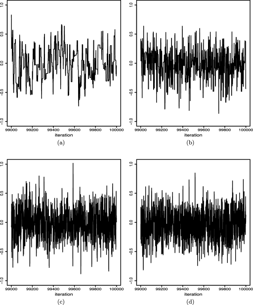
Figure 1: Trace plots of $\beta$ for iterations 9.9e4 through 1e5 of the (a) RW, (b) RSGS, (c) RQGS and (d) GS in the Bayesian linear mixed model example of Section 4.1.

Table 1: Results for the Bayesian linear mixed model example of Section 4.1. Estimates of $\mathrm{E}(\beta|y)$, $\sigma^{2}_{\beta}$ and $\operatorname{Var}(\beta|y)$ are based on $n=10^{5}$; middle columns show half-width of 95% confidence interval ($t_{*}=1.960$) and integrated autocorrelation time (ACT). MSE Ratios are relative to GS, with standard errors given in parentheses. Final column shows estimated ESEJD, with standard error in parentheses

Algorithm	$\bolds{\bar{\beta}_{n}}$	$\bolds{\hat{\sigma}^{2}_{\beta}}$	$\bolds{t_{*}\hat{\sigma}_{\beta}/\sqrt{n}}$	ACT	MSE ratio	$\bolds{\widehat{\mathrm{ESEJD}}}$
RW	$-0.018$	0.794	0.0055	$10.919$	5.55 (0.32)	0.26 (0.0002)
RSGS	$-0.016$	0.243	0.0031	$3.375$	2.07 (0.13)	3.20 (0.0014)
RQGS	$-0.016$	0.071	0.0017	$0.986$	0.98 (0.05)	6.19 (0.0013)
GS	$-0.015$	0.083	0.0018	$1.153$	1.00 (0.00)	6.19 (0.0012)

The differences in the trace plots between the four simulations are reflected in the interval half-width and ACT estimates given in Table 1. For equivalent sample sizes, the RW half-width is nearly two times that of the RSGS and approximately three times as large as those of the GS and RQGS. In addition, the ACTs indicate that nearly eleven RW samples and more than three RSGS samples are required for each random draw from $\pi$ in order to achieve the same level of precision for estimates of $\mathrm{E}(\beta|y)$. On the other hand, each RQGS sample and GS sample is approximately as effective as a random draw.

In order to estimate the MSE of the Monte Carlo estimates, we simulated $m=10^{3}$ independent replications of RW, RSGS, RQGS and GS for $n=10^{4}$ iterations each and took $\bar{\beta}^{*}$ to be an estimate of $\mathrm{E}(\beta|y)$ obtained from $10^{5}$ iterations of the RW chain. The estimated MSE ratios relative to the GS,

$$\frac{\widehat{\operatorname{MSE}}(\bar{\beta}_{n,*})}{\widehat{\operatorname{MSE}}(\bar{\beta}_{n,\mathrm{GS}})}$$

are also given in Table 1 along with standard errors. Notice that ratios greater than one favor GS. Hence, these results are consistent with those above, which suggest that the single block update RW is less efficient than the Gibbs samplers with respect to estimation of $\mathrm{E}(\beta|y)$.

Estimation of the ESEJD is based on the same $m=1000$ independent replications of RW, RSGS, RQGS and GS for $n=10^{4}$ iterations each. The estimates are reported along with standard errors in Table 1. The message here is consistent with the above discussions. The RW appears to be less efficient than the Gibbs samplers in exploring the support of the posterior. Among the Gibbs samplers, there is little difference in the performance quality of the RQGS and GS, whereas both are more efficient than the RSGS.

4.2 A Logit-Normal Mixed Model

Consider the following special case of the mixed model defined in Section 3.1.2. Suppose, conditional on $U=u$, the observations $Y_{ij}$ are independently distributed as $\operatorname{Bernoulli}(p_{ij})$, where $\operatorname{logit}(p_{ij})=\break\beta x_{ij}+u_{i}$ for $j=1,\ldots,m_{i}$ and $i=1,\ldots,k$, where the $x_{ij}$ are covariates. Let the random effects $U_{1},\ldots,U_{k}$ be i.i.d. $\operatorname{Normal}(0,\sigma^{2})$. With the parameters $\theta=(\beta,\sigma^{2})$ treated as fixed, the target density is

$$h(u|y;\theta)$$

$$\quad\propto\exp\Biggl{\{}\sum_{i=1}^{k}\Biggl{[}u_{i}y_{i+}-\sum_{j=1}^{m_{i}}\log\bigl{(}1+e^{\beta x_{ij}+u_{i}}\bigr{)}$$ (21)

$$\hskip 141.5pt\qquad{}-\frac{u_{i}^{2}}{2\sigma^{2}}\Biggr{]}\Biggr{\}},$$

where $y_{i+}=\sum_{j=1}^{m_{i}}y_{ij}$ for $i=1,\ldots,k$.

In Section 3.1.2 we introduced the MHIS, CIS, RQIS and RSIS algorithms. In the current context the conditions of Theorem 5 are satisfied and, hence, those four samplers are uniformly ergodic. In addition, we consider a full-dimensional Metropolis random walk (RW) sampler with normally distributed jump proposals, that is, the proposal density is

$$p\bigl{(}u,u^{*}\bigr{)}\propto\exp\biggl{\{}-\frac{1}{2\tau^{2}}\bigl{\|}u^{*}-u\bigr{\|}^{2}_{2}\biggr{\}},$$ (22)

where $\|\cdot\|_{2}$ denotes the standard Euclidean norm and $\tau^{2}$ is a tuning parameter. Then the following result holds.

Theorem 10

The full-dimensional Metropolis random walk sampler with invariant density (4.2) and proposal density (22) is geometrically ergodic.

We compare the empirical performance of the algorithms in the context of implementing a Monte Carlo EM (MCMC) algorithm. Now at each step the MCEM requires a Monte Carlo approximation to the so-called $Q$-function

$$Q(\theta;\tilde{\theta})=\int{l_{c}(\theta;y,u)h(u|y;\tilde{\theta})\,du},$$

where

$$l_{c}(\theta;y,u)$$

$$\quad=\sum_{i=1}^{k}\sum_{j=1}^{m_{i}}\bigl{[}y_{ij}(\beta x_{ij}+u_{i})-\log\bigl{(}1+e^{\beta x_{ij}+u_{i}}\bigr{)}\bigr{]}$$

$$\qquad{}-\frac{k}{2}\log\bigl{(}\sigma^{2}\bigr{)}-\frac{1}{2\sigma^{2}}\sum_{i=1}^{k}u_{i}^{2}$$

denotes the “complete-data log-likelihood,” what the log-likelihood would be if the random effects were observable. We consider implementation of MCEM in a benchmark data set given by Booth and Hobert [(1999), Table 2], assuming the true parameter value $\theta=(\beta,\sigma^{2})=(5.0,0.5)$. In this data set $x_{ij}=j/15$ for each $j=1,\ldots,m_{i}\equiv 15$, for each $i=1,\ldots,k=10$. Let $\tilde{\theta}=(4.0,1.5)$. We can take as an MCMC approximation of the $Q$-function the sample average of the chain $\{l_{c}(\theta;y,u^{(t)})\}$, that is,

$$Q(\theta;\tilde{\theta})\approx{\overline{l}_{C}}_{n}(\theta;\tilde{\theta}):=\frac{1}{n}\sum_{t=1}^{n}l_{c}\bigl{(}\theta;y,u^{(t)}\bigr{)},$$

where $\{u^{(t)}\dvtx t=1,2,\ldots,n\}$ is a realization of one of our five Markov chains with stationary density $h(u|y;\tilde{\theta})$ as defined by (4.2). For the sake of simplicity we will consider estimating the point $Q(\tilde{\theta};\tilde{\theta})$ rather than the entire function. The mixing conditions on the Markov chain ensure the existence of a CLT for the Monte Carlo error ${\overline{l}_{C}}_{n}(\tilde{\theta};\tilde{\theta})-Q(\tilde{\theta};\tilde{\theta})$ with the variance of the asymptotic normal distribution denoted $\sigma^{2}_{Q}$, which can be consistently estimated with the batch means estimator $\hat{\sigma}^{2}_{Q}$ (Jones et al. (2006)).

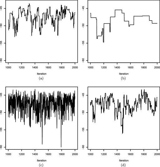
Figure 2: Partial trace plots for the Markov chain $\{l_{c}(\theta;y,u^{(t)})\}$ generated by (a) RW, (b) MHIS, (c) CIS and (d) RSIS in the logit-normal example of Section 4.2.

We implemented MHIS, RW, CIS and RSIS as discussed above—we skip reporting our implementation of RQIS, as it is very similar to CIS in this example—in each case simulating a chain of length $n=10^{6}$ and taking as our initial distribution $U^{(0)}\sim\mathrm{N}_{10}(0,\sigma^{2}I)$. For the Metropolis random walk we drew our jump proposals from a $\mathrm{N}_{10}(0,\tau^{2}I)$, with $\tau^{2}=\sigma^{2}/6$ (this setting determined by trial and error, in order to minimize the autocorrelation in the resulting chain, and yielded an observed acceptance rate of $27.3\%$). A partial trace plot (the second 1000 updates) is shown in panel (a) of Figure 2. Analogous plots for the MHIS and component-wise algorithms appear in the remaining panels.

Consider the trace plots for the four chains. The most striking result is the dreadful performance of the MHIS, shown in panel (b). The RW chain[panel (a)] mixes much faster than the MHIS, but still shows significant autocorrelation. Now RSIS[panel (d)] appears to mix faster than MHIS but is very similar to RW. Finally, the CIS [panel (c)] chain appears to be the best of these four samplers. This suggests that when there is weak dependence between the components of the target distribution, one should use a CWIS instead of a MHIS; recall that Neal and Roberts (2006) reached a similar conclusion for the Metropolis random walk.

In general, the empirical performance of MHIS depends entirely on the “closeness” of the proposal distribution to the target and, clearly, the marginal distribution of the random effects $U$ is not sufficiently similar to the conditional distribution of $U$ given the data. It is worth recalling that, by Theorem 5, the MHIS depicted in panel (b) of Figure 2 is a uniformly ergodic Markov chain. Thus, this example nicely illustrates the perils of over-reliance on asymptotic properties of a sampler, which provide no guarantee of favorable performance in finite-sample implementations.

Table 2: Results for the logit-normal example of Section 4.2. Estimates of $Q(\theta;\tilde{\theta})$, and $\sigma^{2}_{Q}$ at $\theta=\tilde{\theta}=(4.0,1.5)$, are based on $n=10^{6}$; middle columns show half-width of 95% confidence interval ($t_{*}=1.960$) and integrated autocorrelation time (ACT). Rightmost panel shows estimated ESEJD based on $m=10^{3}$ replications, with standard errors in parentheses

Algorithm	$\bolds{\hat{Q}(\theta|\tilde{\theta};y)}$	$\bolds{\hat{\sigma}^{2}_{Q}}$	$\bolds{t_{*}\hat{\sigma}_{Q}/\sqrt{n}}$	ACT	$\bolds{\widehat{\mathrm{ESEJD}}}$
RW	$-47.74$	$203.71$	0.028	$39.37$	0.57 (0.0004)
MHIS	$-47.77$	$2211.16$	0.092	$427.13$	0.13 (0.0015)
CIS	$-47.76$	$19.81$	0.009	$3.87$	4.97 (0.0016)
RSIS	$-47.76$	$258.85$	0.032	$50.08$	0.50 (0.0005)

Consider the simulation results given in Table 2. Using equivalent Monte Carlo sample sizes, the half-width of the interval estimator is roughly the same for RW and RSIS. The half-widths for RW and RSIS are more than 3 times larger than the half-width for CIS. On the other hand, the half-width for MHIS is more than 3 times larger than those of RSIS and RW and more than 10 times larger than that of CIS. The ACTs tell a similar story, RW and RSIS are comparable while MHIS is the worst and CIS is much better.

Estimation of ESEJD is based on the same $m=10^{3}$ independent replications of RW, MHIS, RSIS and CIS for $n=10^{4}$ iterations each. The results here are consistent with the other measures in the above discussion. The performance of MHIS is terrible, while RSIS and RW are comparable and CIS is the best of the four by a wide margin. The fact that RSIS is comparable to RW is surprising. In RSIS only one of the 10 components has a chance to be updated at each step, yet its performance is similar to a chain which updates all of its components about 30% of the time.

5 Concluding Remarks

Outside of the two-variable Gibbs sampler and the random scan Metropolis-within-Gibbs algorithms,there has been little research on convergence rates of component-wise MCMC samplers. This is unfortunate because, as outlined in Section 1, establishing geometric ergodicity is a key step in enabling a practitioner to have as much confidence in the simulation results as if the samples were independent and identically distributed.

Certainly a theme of this paper has been that studying the convergence rates of component-wise samplers formed by composition, that is, $P_{C}$, enables us to establish uniform or geometric ergodicity for other component-wise samplers such as $P_{\mathrm{RQ}}$ and $P_{\mathrm{RS}}$. Indeed, we showed this is true for uniform ergodicity in the general setting and for geometric ergodicity in the two-variable setting. It seems that studying the convergence rates of $P_{\mathrm{RQ}}$ and $P_{\mathrm{RS}}$ should also inform us about the rate of $P_{C}$. Specifically, it is tempting to think that $P_{\mathrm{RS}}$ should converge no faster than $P_{\mathrm{RQ}}$ which should converge no faster than $P_{C}$. Especially in the two-variable setting, we suspect this is the case. Indeed, Tan, Jones and Hobert (2013) study a class of target distributions and show that either both GS and RSGS are geometrically ergodic or neither are.

Another theme has been that component-wiseMCMC methods can be superior to full-dimensional updates. For example, full-dimensional MCMC methods often fail to be geometrically ergodic, but obvious component-wise implementations are. Also, the empirical investigations in Section 4 showed that the finite sample properties of component-wise methods were superior to full-dimensional methods in every case, which matches our observation in so many real data examples; see the references in Section 1. The near ubiquity of component-wise methods in the applied literature suggests that this view is widely held among MCMC practitioners.

References

- Atchadé (2011) {barticle}[mr] \bauthor\bsnmAtchadé, \bfnmYves F.\binitsY. F. (\byear2011). \btitleKernel estimators of asymptotic variance for adaptive Markov chain Monte Carlo. \bjournalAnn. Statist. \bvolume39 \bpages990–1011. \biddoi=10.1214/10-AOS828, issn=0090-5364, mr=2816345 \bptokimsref \endbibitem
- Bédard and Rosenthal (2008) {barticle}[mr] \bauthor\bsnmBédard, \bfnmMylène\binitsM. and \bauthor\bsnmRosenthal, \bfnmJeffrey S.\binitsJ. S. (\byear2008). \btitleOptimal scaling of Metropolis algorithms: Heading toward general target distributions. \bjournalCanad. J. Statist. \bvolume36 \bpages483–503. \biddoi=10.1002/cjs.5550360401, issn=0319-5724, mr=2532248 \bptokimsref \endbibitem
- Booth and Hobert (1999) {barticle}[auto:STB—2013/06/05—13:45:01] \bauthor\bsnmBooth, \bfnmJ. G.\binitsJ. G. and \bauthor\bsnmHobert, \bfnmJ. P.\binitsJ. P. (\byear1999). \btitleMaximizing generalized linear mixed model likelihoods with an automated Monte Carlo EM algorithm. \bjournalJ. R. Stat. Soc. Ser. B Stat. Methodol. \bvolume61 \bpages265–285. \bptokimsref \endbibitem
- Caffo, Jank and Jones (2005) {barticle}[mr] \bauthor\bsnmCaffo, \bfnmBrian S.\binitsB. S., \bauthor\bsnmJank, \bfnmWolfgang\binitsW. and \bauthor\bsnmJones, \bfnmGalin L.\binitsG. L. (\byear2005). \btitleAscent-based Monte Carlo expectation-maximization. \bjournalJ. R. Stat. Soc. Ser. B Stat. Methodol. \bvolume67 \bpages235–251. \biddoi=10.1111/j.1467-9868.2005.00499.x, issn=1369-7412, mr=2137323 \bptokimsref \endbibitem
- Christensen, Møller and Waagepetersen (2001) {barticle}[mr] \bauthor\bsnmChristensen, \bfnmO. F.\binitsO. F., \bauthor\bsnmMøller, \bfnmJ.\binitsJ. and \bauthor\bsnmWaagepetersen, \bfnmR. P.\binitsR. P. (\byear2001). \btitleGeometric ergodicity of Metropolis–Hastings algorithms for conditional simulation in generalized linear mixed models. \bjournalMethodol. Comput. Appl. Probab. \bvolume3 \bpages309–327. \biddoi=10.1023/A:1013779208892, issn=1387-5841, mr=1891114 \bptokimsref \endbibitem
- Coull et al. (2001) {barticle}[mr] \bauthor\bsnmCoull, \bfnmBrent A.\binitsB. A., \bauthor\bsnmHobert, \bfnmJames P.\binitsJ. P., \bauthor\bsnmRyan, \bfnmLouise M.\binitsL. M. and \bauthor\bsnmHolmes, \bfnmLewis B.\binitsL. B. (\byear2001). \btitleCrossed random effect models for multiple outcomes in a study of teratogenesis. \bjournalJ. Amer. Statist. Assoc. \bvolume96 \bpages1194–1204. \biddoi=10.1198/016214501753381841, issn=0162-1459, mr=1946573 \bptokimsref \endbibitem
- Diaconis, Khare and Saloff-Coste (2008) {barticle}[mr] \bauthor\bsnmDiaconis, \bfnmPersi\binitsP., \bauthor\bsnmKhare, \bfnmKshitij\binitsK. and \bauthor\bsnmSaloff-Coste, \bfnmLaurent\binitsL. (\byear2008). \btitleGibbs sampling, exponential families and orthogonal polynomials. \bjournalStatist. Sci. \bvolume23 \bpages151–178. \biddoi=10.1214/07-STS252, issn=0883-4237, mr=2446500 \bptnotecheck related\bptokimsref \endbibitem
- Doss and Hobert (2010) {barticle}[mr] \bauthor\bsnmDoss, \bfnmHani\binitsH. and \bauthor\bsnmHobert, \bfnmJames P.\binitsJ. P. (\byear2010). \btitleEstimation of Bayes factors in a class of hierarchical random effects models using a geometrically ergodic MCMC algorithm. \bjournalJ. Comput. Graph. Statist. \bvolume19 \bpages295–312. \biddoi=10.1198/jcgs.2010.09182, issn=1061-8600, mr=2675092 \bptokimsref \endbibitem
- Flegal, Haran and Jones (2008) {barticle}[mr] \bauthor\bsnmFlegal, \bfnmJames M.\binitsJ. M., \bauthor\bsnmHaran, \bfnmMurali\binitsM. and \bauthor\bsnmJones, \bfnmGalin L.\binitsG. L. (\byear2008). \btitleMarkov chain Monte Carlo: Can we trust the third significant figure? \bjournalStatist. Sci. \bvolume23 \bpages250–260. \biddoi=10.1214/08-STS257, issn=0883-4237, mr=2516823 \bptokimsref \endbibitem
- Flegal and Jones (2010) {barticle}[mr] \bauthor\bsnmFlegal, \bfnmJames M.\binitsJ. M. and \bauthor\bsnmJones, \bfnmGalin L.\binitsG. L. (\byear2010). \btitleBatch means and spectral variance estimators in Markov chain Monte Carlo. \bjournalAnn. Statist. \bvolume38 \bpages1034–1070. \biddoi=10.1214/09-AOS735, issn=0090-5364, mr=2604704 \bptokimsref \endbibitem
- Flegal and Jones (2011) {bincollection}[mr] \bauthor\bsnmFlegal, \bfnmJ. M.\binitsJ. M. and \bauthor\bsnmJones, \bfnmG. L.\binitsG. L. (\byear2011). \btitleImplementing Markov chain Monte Carlo: Estimating with confidence. In \bbooktitleHandbook of Markov Chain Monte Carlo (\beditor\bfnmS. P.\binitsS. P. \bsnmBrooks, \beditor\bfnmA.\binitsA. \bsnmGelman, \beditor\bfnmG. L.\binitsG. L. \bsnmJones and \beditor\bfnmX. L.\binitsX. L. \bsnmMeng, eds.). \bpublisherCRC Press, \blocationBoca Raton, FL. \bptokimsref \endbibitem
- Fort et al. (2003) {barticle}[mr] \bauthor\bsnmFort, \bfnmG.\binitsG., \bauthor\bsnmMoulines, \bfnmE.\binitsE., \bauthor\bsnmRoberts, \bfnmG. O.\binitsG. O. and \bauthor\bsnmRosenthal, \bfnmJ. S.\binitsJ. S. (\byear2003). \btitleOn the geometric ergodicity of hybrid samplers. \bjournalJ. Appl. Probab. \bvolume40 \bpages123–146. \bidissn=0021-9002, mr=1953771 \bptokimsref \endbibitem
- Geyer (1999) {bincollection}[mr] \bauthor\bsnmGeyer, \bfnmC.\binitsC. (\byear1999). \btitleLikelihood inference for spatial point processes. In \bbooktitleStochastic Geometry (Toulouse, 1996) (\beditorO. E. Barndorff-Nielsen, \beditorW. S. Kendall and \beditorM. N. M. van Lieshout, eds.). \bseriesMonographs on Statistics and Applied Probability \bvolume80 \bpages79–140. \bpublisherChapman & Hall/CRC, \blocationBoca Raton, FL. \bidmr=1673118 \bptokimsref \endbibitem
- Hobert (2000) {barticle}[mr] \bauthor\bsnmHobert, \bfnmJames P.\binitsJ. P. (\byear2000). \btitleHierarchical models: A current computational perspective. \bjournalJ. Amer. Statist. Assoc. \bvolume95 \bpages1312–1316. \biddoi=10.2307/2669778, issn=0162-1459, mr=1825284 \bptokimsref \endbibitem
- Hobert (2011) {bincollection}[mr] \bauthor\bsnmHobert, \bfnmJ. P.\binitsJ. P. (\byear2011). \btitleThe data augmentation algorithm: Theory and methodology. In \bbooktitleHandbook of Markov Chain Monte Carlo (\beditor\bfnmS. P.\binitsS. P. \bsnmBrooks, \beditor\bfnmA.\binitsA. \bsnmGelman, \beditor\bfnmG. L.\binitsG. L. \bsnmJones and \beditor\bfnmX. L.\binitsX. L. \bsnmMeng, eds.). \bpublisherCRC Press, \blocationBoca Raton, FL. \bptokimsref \endbibitem
- Hobert and Geyer (1998) {barticle}[mr] \bauthor\bsnmHobert, \bfnmJames P.\binitsJ. P. and \bauthor\bsnmGeyer, \bfnmCharles J.\binitsC. J. (\byear1998). \btitleGeometric ergodicity of Gibbs and block Gibbs samplers for a hierarchical random effects model. \bjournalJ. Multivariate Anal. \bvolume67 \bpages414–430. \biddoi=10.1006/jmva.1998.1778, issn=0047-259X, mr=1659196 \bptokimsref \endbibitem
- Hobert et al. (2002) {barticle}[mr] \bauthor\bsnmHobert, \bfnmJames P.\binitsJ. P., \bauthor\bsnmJones, \bfnmGalin L.\binitsG. L., \bauthor\bsnmPresnell, \bfnmBrett\binitsB. and \bauthor\bsnmRosenthal, \bfnmJeffrey S.\binitsJ. S. (\byear2002). \btitleOn the applicability of regenerative simulation in Markov chain Monte Carlo. \bjournalBiometrika \bvolume89 \bpages731–743. \biddoi=10.1093/biomet/89.4.731, issn=0006-3444, mr=1946508 \bptokimsref \endbibitem
- Jarner and Hansen (2000) {barticle}[mr] \bauthor\bsnmJarner, \bfnmSøren Fiig\binitsS. F. and \bauthor\bsnmHansen, \bfnmErnst\binitsE. (\byear2000). \btitleGeometric ergodicity of Metropolis algorithms. \bjournalStochastic Process. Appl. \bvolume85 \bpages341–361. \biddoi=10.1016/S0304-4149(99)00082-4, issn=0304-4149, mr=1731030 \bptokimsref \endbibitem
- Johnson and Geyer (2012) {barticle}[auto:STB—2013/06/05—13:45:01] \bauthor\bsnmJohnson, \bfnmL. T.\binitsL. T. and \bauthor\bsnmGeyer, \bfnmC. J.\binitsC. J. (\byear2012). \btitleVariable transformation to obtain geometric ergodicity in the random-walk Metropolis algorithm. \bjournalAnn. Statist. \bvolume40 \bpages3050–3076. \bptokimsref \endbibitem
- Johnson and Jones (2010) {barticle}[mr] \bauthor\bsnmJohnson, \bfnmAlicia A.\binitsA. A. and \bauthor\bsnmJones, \bfnmGalin L.\binitsG. L. (\byear2010). \btitleGibbs sampling for a Bayesian hierarchical general linear model. \bjournalElectron. J. Stat. \bvolume4 \bpages313–333. \biddoi=10.1214/09-EJS515, issn=1935-7524, mr=2645487 \bptokimsref \endbibitem
- Johnson, Jones and Neath (2013) {bmisc}[auto:STB—2013/06/05—13:45:01] \bauthor\bsnmJohnson, \bfnmA. A.\binitsA. A., \bauthor\bsnmJones, \bfnmG. L.\binitsG. L. and \bauthor\bsnmNeath, \bfnmR. C.\binitsR. C. (\byear2013). \bhowpublishedSupplement to “Component-Wise Markov Chain Monte Carlo: Uniform and Geometric Ergodicity Under Mixing and Composition.” DOI:\doiurl10.1214/13-STS423SUPP. \bptokimsref \endbibitem
- Jones and Hobert (2001) {barticle}[mr] \bauthor\bsnmJones, \bfnmGalin L.\binitsG. L. and \bauthor\bsnmHobert, \bfnmJames P.\binitsJ. P. (\byear2001). \btitleHonest exploration of intractable probability distributions via Markov chain Monte Carlo. \bjournalStatist. Sci. \bvolume16 \bpages312–334. \biddoi=10.1214/ss/1015346317, issn=0883-4237, mr=1888447 \bptokimsref \endbibitem
- Jones and Hobert (2004) {barticle}[mr] \bauthor\bsnmJones, \bfnmGalin L.\binitsG. L. and \bauthor\bsnmHobert, \bfnmJames P.\binitsJ. P. (\byear2004). \btitleSufficient burn-in for Gibbs samplers for a hierarchical random effects model. \bjournalAnn. Statist. \bvolume32 \bpages784–817. \biddoi=10.1214/009053604000000184, issn=0090-5364, mr=2060178 \bptokimsref \endbibitem
- Jones, Roberts and Rosenthal (2013) {bmisc}[auto:STB—2013/06/05—13:45:01] \bauthor\bsnmJones, \bfnmG. L.\binitsG. L., \bauthor\bsnmRoberts, \bfnmG. O.\binitsG. O. and \bauthor\bsnmRosenthal, \bfnmJ. S.\binitsJ. S. (\byear2013). \bhowpublishedConvergence of conditional Metropolis–Hastings samplers. J. Appl. Probab. To appear. \bptokimsref \endbibitem
- Jones et al. (2006) {barticle}[mr] \bauthor\bsnmJones, \bfnmGalin L.\binitsG. L., \bauthor\bsnmHaran, \bfnmMurali\binitsM., \bauthor\bsnmCaffo, \bfnmBrian S.\binitsB. S. and \bauthor\bsnmNeath, \bfnmRonald\binitsR. (\byear2006). \btitleFixed-width output analysis for Markov chain Monte Carlo. \bjournalJ. Amer. Statist. Assoc. \bvolume101 \bpages1537–1547. \biddoi=10.1198/016214506000000492, issn=0162-1459, mr=2279478 \bptokimsref \endbibitem
- Łatuszynski, Roberts and Rosenthal (2013) {barticle}[mr] \bauthor\bsnmŁatuszynski, \bfnmK.\binitsK., \bauthor\bsnmRoberts, \bfnmGareth O.\binitsG. O. and \bauthor\bsnmRosenthal, \bfnmJeffrey S.\binitsJ. S. (\byear2013). \btitleAdaptive Gibbs samplers and related MCMC methods. \bjournalAnn. Appl. Probab. \bvolume23 \bpages66–98. \bptokimsref \endbibitem
- Lee et al. (2013) {bmisc}[auto:STB—2013/06/05—13:45:01] \bauthor\bsnmLee, \bfnmK. J.\binitsK. J., \bauthor\bsnmJones, \bfnmG. L.\binitsG. L., \bauthor\bsnmCaffo, \bfnmB. S.\binitsB. S. and \bauthor\bsnmBassett, \bfnmS.\binitsS. (\byear2013). \bhowpublishedSpatial Bayesian variable selection models on functional magnetic resonance imaging time-series data. Preprint. \bptokimsref \endbibitem
- Marchev and Hobert (2004) {barticle}[mr] \bauthor\bsnmMarchev, \bfnmDobrin\binitsD. and \bauthor\bsnmHobert, \bfnmJames P.\binitsJ. P. (\byear2004). \btitleGeometric ergodicity of van Dyk and Meng’s algorithm for the multivariate Student’s model. \bjournalJ. Amer. Statist. Assoc. \bvolume99 \bpages228–238. \biddoi=10.1198/016214504000000223, issn=0162-1459, mr=2054301 \bptokimsref \endbibitem
- McCulloch (1997) {barticle}[mr] \bauthor\bsnmMcCulloch, \bfnmCharles E.\binitsC. E. (\byear1997). \btitleMaximum likelihood algorithms for generalized linear mixed models. \bjournalJ. Amer. Statist. Assoc. \bvolume92 \bpages162–170. \biddoi=10.2307/2291460, issn=0162-1459, mr=1436105 \bptokimsref \endbibitem
- Mengersen and Tweedie (1996) {barticle}[mr] \bauthor\bsnmMengersen, \bfnmK. L.\binitsK. L. and \bauthor\bsnmTweedie, \bfnmR. L.\binitsR. L. (\byear1996). \btitleRates of convergence of the Hastings and Metropolis algorithms. \bjournalAnn. Statist. \bvolume24 \bpages101–121. \biddoi=10.1214/aos/1033066201, issn=0090-5364, mr=1389882 \bptokimsref \endbibitem
- Meyn and Tweedie (1993) {bbook}[mr] \bauthor\bsnmMeyn, \bfnmS. P.\binitsS. P. and \bauthor\bsnmTweedie, \bfnmR. L.\binitsR. L. (\byear1993). \btitleMarkov Chains and Stochastic Stability. \bpublisherSpringer, \blocationLondon. \bidmr=1287609 \bptokimsref \endbibitem
- Meyn and Tweedie (1994) {barticle}[mr] \bauthor\bsnmMeyn, \bfnmSean P.\binitsS. P. and \bauthor\bsnmTweedie, \bfnmR. L.\binitsR. L. (\byear1994). \btitleComputable bounds for geometric convergence rates of Markov chains. \bjournalAnn. Appl. Probab. \bvolume4 \bpages981–1011. \bidissn=1050-5164, mr=1304770 \bptokimsref \endbibitem
- Neal and Roberts (2006) {barticle}[mr] \bauthor\bsnmNeal, \bfnmPeter\binitsP. and \bauthor\bsnmRoberts, \bfnmGareth\binitsG. (\byear2006). \btitleOptimal scaling for partially updating MCMC algorithms. \bjournalAnn. Appl. Probab. \bvolume16 \bpages475–515. \biddoi=10.1214/105051605000000791, issn=1050-5164, mr=2244423 \bptokimsref \endbibitem
- Neath (2013) {bincollection}[auto:STB—2013/06/05—13:45:01] \bauthor\bsnmNeath, \bfnmR. C.\binitsR. C. (\byear2013). \btitleOn convergence properties of the Monte Carlo EM algorithm. In \bbooktitleAdvances in Modern Statistical Theory and Applications: A Festschrift in Honor of Morris L. Eaton (\beditor\bfnmG. L.\binitsG. L. \bsnmJones and \beditor\bfnmX.\binitsX. \bsnmShen, eds.). \bnoteTo appear. \bptokimsref \endbibitem
- Papaspiliopoulos and Roberts (2008) {barticle}[mr] \bauthor\bsnmPapaspiliopoulos, \bfnmOmiros\binitsO. and \bauthor\bsnmRoberts, \bfnmGareth\binitsG. (\byear2008). \btitleStability of the Gibbs sampler for Bayesian hierarchical models. \bjournalAnn. Statist. \bvolume36 \bpages95–117. \biddoi=10.1214/009053607000000749, issn=0090-5364, mr=2387965 \bptokimsref \endbibitem
- Robert (1995) {barticle}[mr] \bauthor\bsnmRobert, \bfnmChristian P.\binitsC. P. (\byear1995). \btitleConvergence control methods for Markov chain Monte Carlo algorithms. \bjournalStatist. Sci. \bvolume10 \bpages231–253. \bidissn=0883-4237, mr=1390517 \bptokimsref \endbibitem
- Roberts and Polson (1994) {barticle}[mr] \bauthor\bsnmRoberts, \bfnmGareth O.\binitsG. O. and \bauthor\bsnmPolson, \bfnmNicholas G.\binitsN. G. (\byear1994). \btitleOn the geometric convergence of the Gibbs sampler. \bjournalJ. R. Stat. Soc. Ser. B Stat. Methodol. \bvolume56 \bpages377–384. \bidissn=0035-9246, mr=1281941 \bptokimsref \endbibitem
- Roberts and Rosenthal (1997) {barticle}[mr] \bauthor\bsnmRoberts, \bfnmGareth O.\binitsG. O. and \bauthor\bsnmRosenthal, \bfnmJeffrey S.\binitsJ. S. (\byear1997). \btitleGeometric ergodicity and hybrid Markov chains. \bjournalElectron. Commun. Probab. \bvolume2 \bpages13–25 (electronic). \biddoi=10.1214/ECP.v2-981, issn=1083-589X, mr=1448322 \bptokimsref \endbibitem
- Roberts and Rosenthal (1998) {barticle}[mr] \bauthor\bsnmRoberts, \bfnmGareth O.\binitsG. O. and \bauthor\bsnmRosenthal, \bfnmJeffrey S.\binitsJ. S. (\byear1998). \btitleTwo convergence properties of hybrid samplers. \bjournalAnn. Appl. Probab. \bvolume8 \bpages397–407. \biddoi=10.1214/aoap/1028903533, issn=1050-5164, mr=1624941 \bptokimsref \endbibitem
- Roberts and Rosenthal (1999) {barticle}[mr] \bauthor\bsnmRoberts, \bfnmGareth O.\binitsG. O. and \bauthor\bsnmRosenthal, \bfnmJeffrey S.\binitsJ. S. (\byear1999). \btitleConvergence of slice sampler Markov chains. \bjournalJ. R. Stat. Soc. Ser. B Stat. Methodol. \bvolume61 \bpages643–660. \biddoi=10.1111/1467-9868.00198, issn=1369-7412, mr=1707866 \bptokimsref \endbibitem
- Roberts and Rosenthal (2001) {barticle}[mr] \bauthor\bsnmRoberts, \bfnmGareth O.\binitsG. O. and \bauthor\bsnmRosenthal, \bfnmJeffrey S.\binitsJ. S. (\byear2001). \btitleMarkov chains and de-initializing processes. \bjournalScand. J. Stat. \bvolume28 \bpages489–504. \biddoi=10.1111/1467-9469.00250, issn=0303-6898, mr=1858413 \bptokimsref \endbibitem
- Roberts and Rosenthal (2004) {barticle}[mr] \bauthor\bsnmRoberts, \bfnmGareth O.\binitsG. O. and \bauthor\bsnmRosenthal, \bfnmJeffrey S.\binitsJ. S. (\byear2004). \btitleGeneral state space Markov chains and MCMC algorithms. \bjournalProbab. Surv. \bvolume1 \bpages20–71. \biddoi=10.1214/154957804100000024, issn=1549-5787, mr=2095565 \bptokimsref \endbibitem
- Roberts and Sahu (1997) {barticle}[mr] \bauthor\bsnmRoberts, \bfnmG. O.\binitsG. O. and \bauthor\bsnmSahu, \bfnmS. K.\binitsS. K. (\byear1997). \btitleUpdating schemes, correlation structure, blocking and parameterization for the Gibbs sampler. \bjournalJ. R. Stat. Soc. Ser. B Stat. Methodol. \bvolume59 \bpages291–317. \biddoi=10.1111/1467-9868.00070, issn=0035-9246, mr=1440584 \bptokimsref \endbibitem
- Roberts and Tweedie (1996) {barticle}[mr] \bauthor\bsnmRoberts, \bfnmG. O.\binitsG. O. and \bauthor\bsnmTweedie, \bfnmR. L.\binitsR. L. (\byear1996). \btitleGeometric convergence and central limit theorems for multidimensional Hastings and Metropolis algorithms. \bjournalBiometrika \bvolume83 \bpages95–110. \biddoi=10.1093/biomet/83.1.95, issn=0006-3444, mr=1399158 \bptokimsref \endbibitem
- Román (2012) {bmisc}[auto:STB—2013/06/05—13:45:01] \bauthor\bsnmRomán, \bfnmJ. C.\binitsJ. C. (\byear2012). \bhowpublishedConvergence analysis of block Gibbs samplers for Bayesian general linear mixed models. Ph.D. thesis, Dept. Statistics, Univ. Florida. \bptokimsref \endbibitem
- Román and Hobert (2012) {barticle}[auto:STB—2013/06/05—13:45:01] \bauthor\bsnmRomán, \bfnmJ. C.\binitsJ. C. and \bauthor\bsnmHobert, \bfnmJ. P.\binitsJ. P. (\byear2012). \btitleConvergence analysis of the Gibbs sampler for Bayesian general linear mixed models with improper priors. \bjournalAnn. Statist. \bvolume40 \bpages2823–2849. \bptokimsref \endbibitem
- Rosenthal (1995) {barticle}[mr] \bauthor\bsnmRosenthal, \bfnmJeffrey S.\binitsJ. S. (\byear1995). \btitleMinorization conditions and convergence rates for Markov chain Monte Carlo. \bjournalJ. Amer. Statist. Assoc. \bvolume90 \bpages558–566. \bidissn=0162-1459, mr=1340509 \bptokimsref \endbibitem
- Rosenthal (1996) {barticle}[auto:STB—2013/06/05—13:45:01] \bauthor\bsnmRosenthal, \bfnmJ. S.\binitsJ. S. (\byear1996). \btitleAnalysis of the Gibbs sampler for a model related to James–Stein estimators. \bjournalStatist. Comput. \bvolume6 \bpages269–275. \bptokimsref \endbibitem
- Rosenthal (2011) {bincollection}[mr] \bauthor\bsnmRosenthal, \bfnmJ. S.\binitsJ. S. (\byear2011). \btitleOptimal proposal distributions and adaptive MCMC. In \bbooktitleHandbook of Markov Chain Monte Carlo (\beditor\bfnmS. P.\binitsS. P. \bsnmBrooks, \beditor\bfnmA.\binitsA. \bsnmGelman, \beditor\bfnmG. L.\binitsG. L. \bsnmJones and \beditor\bfnmX. L.\binitsX. L. \bsnmMeng, eds.). \bpublisherCRC Press, \blocationBoca Raton, FL. \bptokimsref \endbibitem
- Roy and Hobert (2007) {barticle}[mr] \bauthor\bsnmRoy, \bfnmVivekananda\binitsV. and \bauthor\bsnmHobert, \bfnmJames P.\binitsJ. P. (\byear2007). \btitleConvergence rates and asymptotic standard errors for Markov chain Monte Carlo algorithms for Bayesian probit regression. \bjournalJ. R. Stat. Soc. Ser. B Stat. Methodol. \bvolume69 \bpages607–623. \biddoi=10.1111/j.1467-9868.2007.00602.x, issn=1369-7412, mr=2370071 \bptokimsref \endbibitem
- Tan and Hobert (2009) {barticle}[mr] \bauthor\bsnmTan, \bfnmAixin\binitsA. and \bauthor\bsnmHobert, \bfnmJames P.\binitsJ. P. (\byear2009). \btitleBlock Gibbs sampling for Bayesian random effects models with improper priors: Convergence and regeneration. \bjournalJ. Comput. Graph. Statist. \bvolume18 \bpages861–878. \biddoi=10.1198/jcgs.2009.08153, issn=1061-8600, mr=2598033 \bptokimsref \endbibitem
- Tan, Jones and Hobert (2013) {bincollection}[auto:STB—2013/06/05—13:45:01] \bauthor\bsnmTan, \bfnmA.\binitsA., \bauthor\bsnmJones, \bfnmG. L.\binitsG. L. and \bauthor\bsnmHobert, \bfnmJ. P.\binitsJ. P. (\byear2013). \btitleOn the geometric ergodicity of two-variable Gibbs samplers. In \bbooktitleAdvances in Modern Statistical Theory and Applications: A Festschrift in Honor of Morris L. Eaton (\beditor\bfnmG. L.\binitsG. L. \bsnmJones and \beditor\bfnmX.\binitsX. \bsnmShen, eds.). \bnoteTo appear. \bptokimsref \endbibitem
- Tanner and Wong (1987) {barticle}[mr] \bauthor\bsnmTanner, \bfnmMartin A.\binitsM. A. and \bauthor\bsnmWong, \bfnmWing Hung\binitsW. H. (\byear1987). \btitleThe calculation of posterior distributions by data augmentation (with discussion). \bjournalJ. Amer. Statist. Assoc. \bvolume82 \bpages528–550. \bidissn=0162-1459, mr=0898357 \bptokimsref \endbibitem
- Tierney (1994) {barticle}[mr] \bauthor\bsnmTierney, \bfnmLuke\binitsL. (\byear1994). \btitleMarkov chains for exploring posterior distributions (with discussion). \bjournalAnn. Statist. \bvolume22 \bpages1701–1762. \biddoi=10.1214/aos/1176325750, issn=0090-5364, mr=1329166 \bptokimsref \endbibitem