Non-Gaussianity in a Matter Bounce

Abstract

A nonsingular bouncing cosmology in which the scales of interest today exit the Hubble radius in a matter-dominated contracting phase yields an alternative to inflation for producing a scale-invariant spectrum of adiabatic cosmological fluctuations. In this paper we identify signatures in the non-Gaussianities of the fluctuations which are specific to this scenario and allow it to be distinguished from the results of inflationary models.

I Introduction

One of the problems of the inflationary scenario Guth, the current paradigm of early universe cosmology, is the presence of an initial singularity. Such a singularity is unavoidable if inflation is obtained from matter scalar fields in the context of the Einstein action for space-time Borde. As a consequence, there has been a lot of interest in resolving the singularity by means of quantum gravity effects or effective field theory techniques.

A successful resolution of the cosmological singularity may lead to a non-singular bouncing cosmology. Such non-singular bounces were proposed a long time ago Tolman. They were studied in models motivated by approaches to quantum gravity such as the Pre-Big-Bang model PBB, higher derivative gravity actions (see e.g. Markov; nonsing; Tsujik; Biswas), brane world scenarios Varun or loop quantum cosmology LQC. Nonsingular bounces may also emerge from non-perturbative superstring theory, as has been investigated using tools such as $c=1$ matrix theory Joanna or the AdS/CFT correspondence Sethi; Das. String gas cosmology BV, an approach to string cosmology in which the temperature of the universe is non-singular, may also be embedded in a bouncing cosmology, as realized e.g. in Biswas2. Finally, non-singular bounces may be studied using effective field theory techniques by introducing a curvature term Peter or matter fields violating the key energy conditions, for example non-conventional fluids prequintom; Bozza, or quintom matter quintom. A specific realization of such a quintom bounce occurs in the Lee-Wick cosmology studied in LW

In the context of studies of bouncing cosmologies it has been realized that fluctuations which are generated as quantum vacuum perturbations and exit the Hubble radius during a matter-dominated contracting phase lead to a scale-invariant spectrum of cosmological fluctuations today FB2; Wands; Wands2; Pinto (see also Starob). This yields an alternative to cosmological inflation in explaining the current observational data. We will call this scenario the “matter bounce”.

It is important to study ways to distinguish the predictions of the matter bounce from those of the standard inflationary paradigm. One criterion is the tensor to scalar ratio which is typically large for a matter bounce Wands2; LW. In this Letter, we study the distinctive signatures of the matter bounce in the non-Gaussianities of the spectrum of cosmological fluctuations.

We find that the amplitude of the non-Gaussianities is larger than in simple inflationary models. This is due to the fact that the fluctuations grow on super-Hubble scales in a contracting universe. This growth also leads to a specific signature in the shape of the non-Gaussianities which emerges since it is different solutions of the fluctuation equation which dominate the spectrum compared to the case of standard inflation. Both the amplitude and shape of the three-point function are predicted independent of any free parameters.

In the following, we first review the key new features which effect the evolution of cosmological fluctuations in contracting backgrounds, specifically in the case of the matter bounce. Then, we turn to the calculation of the non-Gaussianity function $f_{NL}$ and compare our result with the predictions of simple slow-roll inflation models.

II Fluctuations in a Contracting Universe

To discuss cosmological fluctuations, we write the metric in the following form (see MFB for a detailed exposition of the theory of cosmological perturbations and RHBrev1 for an overview):

$$ds^{2}\,=\,a^{2}(\eta)\bigl[(1+2\Phi)d\eta^{2}-(1-2\Phi)d{\bf{x}}^{2}\bigr]\,,$$ (1)

where $\eta$ is conformal time and $\Phi(x,\eta)$ describes the metric fluctuations .

To follow fluctuations from the contracting to the expanding phase we will be following most of the literature and will use the variable $\zeta$ which describes the curvature fluctuations in co-moving coordinates. If we take matter to be a scalar field $\varphi$, then $\zeta$ is given by

$$\zeta\,=\,\bigl(\frac{a}{z}\delta\varphi+\Phi\bigr)\,,$$ (2)

where

$$z\,=\,a\frac{\varphi^{\prime}}{\cal{H}}\,,$$ (3)

a prime indicating a derivative with respect to conformal time, and ${\cal H}$ standing for the Hubble expansion rate in conformal time.

The variable $\zeta$ is closely related to the Sasaki-Mukhanov variable Sasaki; Mukh in terms of which the action for cosmological perturbations has canonical kinetic term:

$$v\,=\,z\zeta\,,$$ (4)

The equation of motion for the Fourier mode $v_{k}$ of $v$ is

$$v_{k}^{{}^{\prime\prime}}+\bigl(k^{2}-\frac{z^{{}^{\prime\prime}}}{z}\bigr)v_{k}\,=\,0\,.$$ (5)

If the equation of state of the background is time-independent, then $z\sim a$ and hence the negative square mass term in (5) is $H^{2}$. Thus, on length scales smaller than the Hubble radius, the solutions of (5) are oscillating, whereas on larger scales they are frozen in, and their amplitude depends on the time evolution of $z$.

On super-Hubble scales, the equation of motion (5) for $v_{k}$ in a universe which is contracting or expanding as a power $p$ of physical time $t$, i.e.

$$a(t)\,\sim\,t^{p}\,,$$ (6)

becomes

$$v^{{}^{\prime\prime}}_{k}\,=\,\frac{p(2p-1)}{(p-1)^{2}}\eta^{-2}v_{k}\,,$$ (7)

which has solutions

$$v(\eta)\,\sim\,\eta^{\alpha}$$ (8)

with

$$\alpha\,=\,\frac{1}{2}\pm\nu\,\,\,\,,\,\,\,\,\nu\,=\,\frac{1}{2}\frac{1-3p}{1-p}\,.$$ (9)

In the case of an exponentially expanding universe we must take the $p\rightarrow\infty$ limit of the above solutions. Hence, the solutions for $\alpha$ are $\alpha=3/2$ and $\alpha=-1/2$. The scale factor $a$ is proportional to $\eta^{-1}$. Hence

$$\zeta(\eta)\,=\,c_{1}\eta^{3}+c_{2}\,,$$ (10)

where $c_{1}$ and $c_{2}$ are constants. Since $\eta\rightarrow 0$ as $t\rightarrow\infty$, it is the constant mode which dominates. This leads to the well-known result that the fluctuations of $\zeta$ are constant on super-Hubble scales. This also leads to the conclusion that the power spectrum of $\zeta$ from quantum vacuum perturbations which are initially on sub-Hubble scales is scale-invariant since

$$P_{\zeta}(k,\eta)\, \equiv \,\frac{k^{3}}{12\pi^{2}}|\zeta_{k}(\eta)|^{2}$$ (11)

$$\sim k^{3}|\zeta_{k}(\eta_{H}(k))|^{2}$$

$$\sim k^{3}|v_{k}(\eta_{H}(k)|^{2}a^{-2}(\eta_{H}(k))\,\sim\,k^{3}k^{-1}k^{-2}$$

$$\sim \,{\rm const}\,,$$

making use of the quantum vacuum normalization and the Hubble radius crossing condition.

In the case of a matter-dominated contraction we have $\nu=-3/2$ and hence

$$v_{k}(\eta)\,=c_{1}\eta^{2}+c_{2}\eta^{-1}\,,$$ (12)

where $c_{1}$ and $c_{2}$ are again constants. The $c_{1}$ mode is the mode for which $\zeta$ is constant on super-Hubble scales. However, in a contracting universe it is the $c_{2}$ mode which dominates and leads to a scale-invariant spectrum Wands; FB2; Wands2:

$$P_{\zeta}(k,\eta)\, \sim k^{3}|v_{k}(\eta)^{2}a^{-2}(\eta)$$ (13)

$$\sim \,k^{3}|v_{k}(\eta_{H}(k))|^{2}\bigl(\frac{\eta_{H}(k)}{\eta}\bigr)^{2}\,\sim\,k^{3-1-2}$$

$$\sim \,{\rm const}\,,$$

once again using the scaling of the dominant mode of $v_{k}$, the Hubble radius crossing condition $\eta_{H}(k)\sim k^{-1}$, and the vacuum spectrum at Hubble radius crossing.

III Non-Gaussianities in the Matter Bounce

III.1 Formalism

In this section we will consider non-Gaussianities in the matter bounce model. Specifically, we will focus on the amplitude and shape of the three-point function and on the function $f_{NL}$ which is commonly used to describe the leading-order non-Gaussianities.

Non-Gaussianities in single field inflation models were first considered in Wise; Hodges; Salopek; Srednicki; Gangui; KomatsuSpergel and in more detail in Bartolo in the context of single field slow-roll inflation models and it was concluded that the non-Gaussianities would be small. That larger non-Gaussianities can be obtained in multi-field inflation models or DBI inflation models was realized in multifield and Tong, respectively. An elegant formalism for calculating non-Gaussianities was presented in Maldacena and extended to the case of generalized inflation models in Chen. For a comprehensive review of non-Gaussianities the reader is referred to Komatsu.

The presence of interactions in the Lagrangian leads to non-Gaussianities. We will study them following the formalism established in Maldacena. It is easiest to work in the interaction picture, in which the three-point function to leading order in the interaction coupling constant is given by

$$<\zeta(t,\vec{k}_{1})\zeta(t,\vec{k}_{2})\zeta(t,\vec{k}_{3})>$$ (14)

$$\,\,\,\,=\,i\int_{t_{i}}^{t}dt^{\prime}<[\zeta(t,\vec{k}_{1})\zeta(t,\vec{k}_{2})\zeta(t,\vec{k}_{3}),{L}_{int}(t^{\prime})]>~,$$

where $t_{i}$ corresponds to the initial time before which there are any non-Gaussianities. The square parentheses indicate the commutator, and $L_{int}$ is the interaction Lagrangian (the integral over space of the interaction Lagrangian density ${\cal L}$ given below).

To calculate the non-Gaussianities in the function $\zeta$, we require the Lagrangian density for $\zeta$ to cubic order. This has been derived in Maldacena and takes the form

$${\cal L}_{3}\, = \,(\epsilon^{2}-\frac{\epsilon^{3}}{2})a^{3}\zeta\dot{\zeta}^{2}+\epsilon^{2}a\zeta(\partial\zeta)^{2}-2\epsilon^{2}a^{3}\dot{\zeta}(\partial\zeta)(\partial\chi)$$ (15)

$$+\frac{\epsilon^{3}}{2}a^{3}\zeta(\partial_{i}\partial_{j}\chi)^{2}+f(\zeta)\frac{\delta{\cal L}_{2}}{\delta\zeta}|_{1}~,$$

where we define $\chi\equiv\partial^{-2}\dot{\zeta}$ and $\partial^{-2}$ is the inverse Laplacian. The function $f$ in the last term is

$$f(\zeta)\, = \,\frac{1}{4{\cal H}^{2}}(\partial\zeta)^{2}-\frac{1}{4{\cal H}^{2}}\partial^{-2}\partial_{i}\partial_{j}(\partial_{i}\zeta\partial_{j}\zeta)$$ (16)

$$-\frac{a}{{\cal H}}\zeta\dot{\zeta}-\frac{\epsilon a}{2{\cal H}}\partial_{i}\zeta\partial_{i}\partial^{-2}\dot{\zeta}$$

$$+\frac{\epsilon a}{2{\cal H}}\partial^{-2}\partial_{i}\partial_{j}(\partial_{i}\partial^{-2}\dot{\zeta}\partial_{j}\zeta)~,$$

and $\epsilon$ is given by

$$\epsilon\,\equiv\,-\frac{{\dot{H}}}{H^{2}}\,.$$ (17)

In inflationary cosmology, $\epsilon$ is the slow-roll parameter and is generally much smaller than order unity, whereas in our bouncing cosmology

$$\epsilon\,=\,\frac{3}{2}(1+w)\,=\,\frac{3}{2}$$ (18)

in the contracting phase ($w$ is the equation of state parameter).

In the standard cosmological model which describes a universe which was expanding starting from an inflationary phase, $\zeta$ is a constant on scales larger than the Hubble radius. On these scales, the spatial derivatives are negligible, and thus one sees from (16) that the interaction Lagrangian vanishes. Hence, the integration in (15) runs only up to the time of Hubble radius crossing in the inflationary phase, i.e. one must just consider the non-linear growth of $\zeta$ inside the Hubble radius. However, in a contracting universe $\zeta$ grows on scales larger than the Hubble radius. Hence, the integration in (15) is dominated by times when the scale is super-Hubble (until the bounce time, after which $\zeta$ stops growing on super-Hubble scales). As we show below, this leads to a difference in the shape of the non-Gaussianities. One way to see this is to note that $\zeta$ is oscillating on scales smaller than the Hubble radius, whereas the oscillations are frozen out on super-Hubble scales and the growth of $\zeta$ in the contracting phase occurs as the increase in the amplitude of a frozen wave perturbation. The very different time dependence of $\zeta$ on the scales that dominate the integral (15) leads to a quite different scaling of the integrals, and hence to a different shape of the non-Gaussianities.

There is another important difference between a bouncing cosmology and the inflationary model. In simple single field slow-roll inflation models the cubic Lagrangian is suppressed by the slow-roll parameter $\epsilon\ll 1$ and so the terms proportional to $\epsilon^{3}$ in Eq. (15) can always be neglected. However, in a bouncing cosmology such as the matter bounce these terms contribute at the same order. Moreover, in inflationary cosmology the function $f(\zeta)$ is dominated by the first two terms in Eq. (16) because on large scales $\zeta$ is conserved and thus $\dot{\zeta}=0$ for the dominant mode. In contrast, in the matter bounce it is the last three terms in Eq. (16) which are dominant since the dominant mode of $\zeta$ is growing as $\eta^{-3}$. Since different terms dominate, we will get a different shape of the non-Gaussianities.

The three-point function can be expressed in the following general form:

$$<\zeta(\vec{k}_{1})\zeta(\vec{k}_{2})\zeta(\vec{k}_{3})>\, = \,(2\pi)^{7}\delta(\sum\vec{k}_{i})\frac{P_{\zeta}^{2}}{\prod k_{i}^{3}}$$ (19)

$$\times{\cal A}(\vec{k}_{1},\vec{k}_{2},\vec{k}_{3})~,$$

where $k_{i}=|\vec{k}_{i}|$ and ${\cal A}$ is the shape function whose amplitude is (in the case of “local” non-Gaussianities) characterized by the non-linearity parameter $f_{NL}$, where

$$\zeta\,=\,\zeta_{g}(x)+\frac{3}{5}f_{NL}\zeta_{g}^{2}~,$$ (20)

and $\zeta_{g}(x)$ is the linear (and hence Gaussian) part of $\zeta$. More generally, in momentum space the amplitude ${\cal|B|}_{NL}$ of the non-Gaussianities can be described by

$${\cal|B|}_{NL}(\vec{k}_{1},\vec{k}_{2},\vec{k}_{3})\,=\,\frac{10}{3}\frac{{\cal A}(\vec{k}_{1},\vec{k}_{2},\vec{k}_{3})}{\sum_{i}k_{i}^{3}}~.$$ (21)

As a last preliminary, we note that in the Lagrangian formalism, the curvature perturbation variable $\zeta$ in Fourier space can be canonically expressed as

$$\zeta(\eta,\vec{k})\,=\,u_{k}(\eta){a}^{\dagger}_{\vec{k}}+u_{k}^{*}(\eta)a_{-\vec{k}}$$ (22)

with the matter contracting phase mode functions

$$u_{k}(\eta)\,=\,A\frac{i[1-ik(\eta-\tilde{\eta}_{B})]}{\sqrt{2k^{3}}(\eta-\tilde{\eta}_{B})^{3}}\exp[ik(\eta-\tilde{\eta}_{B})]~,$$ (23)

where $\tilde{\eta}_{B}$ is the conformal time when the singularity would occur if the matter contracting phase would continue to arbitrary densities. The creation and annihilation operators $a$ and $a^{\dagger}$ obey the standard canonical commutation relations. The amplitude $A$ is determined from the quantum vacuum conditions at Hubble radius crossing in the contracting phase. This amplitude determines the power spectrum of $\zeta$. If we factor out the amplitude and the factor of $k^{-3/2}$, we can define the following rescaled mode functions:

$$X_{k}(\eta)\,\equiv\,\frac{1-ik(\eta-\tilde{\eta}_{B})}{(\eta-\tilde{\eta}_{B})^{3}}e^{ik(\eta-\tilde{\eta}_{B})}~.$$ (24)

III.2 Contributions to Non-Gaussianity in the Matter Bounce

In the following we insert the cubic interaction Lagrangian (15) into Eq. (14) and calculate the vacuum expectation value of the three-point function contributed by the interaction terms one by one. We evaluate the non-Gaussianity at the bounce time $\eta_{B}$.

However, before doing that we employ the same trick as used in Maldacena: In order to cancel the last term in Eq. (15), we make the following field redefinition

$$\zeta\,\rightarrow\,\zeta-f(\zeta)~.$$ (25)

Inserting this field redefinition into (14) we find two terms: the three point function of the rescaled field $\zeta$ on one hand, and terms in which one factor of $\zeta$ has been replaced by $f(\zeta)$ on the other hand.

To compute the first term, we evaluate the right hand side of (14) with an interaction Lagrangian which does not contain the last term in (15). Below, we consider the contributions of each remaining term in (15). The second term is called the “field redefinition term”. It does not involve any integration over time.

Now we consider the individual terms:

• Contribution from the field redefinition

  Since on large scales the first two terms of $f(\zeta)$ can be neglected, we only need to consider the other three. Note that this is precisely the opposite of what happens in the inflationary paradigm where it is the first two terms which dominate. As a consequence of this difference, the field redefinition term leads to a very different shape function.

  Moreover, from the solution of the equation of motion for $\zeta$ one can see that there is an approximate relation

  $$\dot{\zeta}\,\simeq\,-\frac{3}{2}H\zeta$$ (26)

  valid on scales larger than the Hubble radius. Therefore, we obtain the following approximate form of the redefinition term in momentum space,

  $$\zeta(\vec{k})\, \rightarrow \,\zeta(\vec{k})-\int\frac{dk^{\prime 3}}{(2\pi)^{3}}\{\frac{3}{2}+\frac{9}{8}\frac{\vec{k}^{\prime}\cdot(\vec{k}-\vec{k}^{\prime})}{k^{\prime 2}}$$ (27)

  $$- \,\frac{9}{8}\frac{(\vec{k}\cdot\vec{k}^{\prime})(\vec{k}\cdot(\vec{k}-\vec{k}^{\prime}))}{k^{2}k^{\prime 2}}\}{\zeta(\vec{k}^{\prime})\zeta(\vec{k}-\vec{k}^{\prime})}~,$$

  The corresponding shape function is given by (in this and the following formulas we keep the factor of $\epsilon$ explicit since it will allow us to understand at which order in $\epsilon$ the key differences in shape compared to simple slow-roll single field inflation models arise)

  $${\cal A}_{red}\, = \,-\frac{\epsilon}{2}\sum k_{i}^{3}-\frac{\epsilon^{2}}{32\prod k_{i}^{2}}\bigg\{\sum_{i\neq j}k_{i}^{7}k_{j}^{2}+\sum_{i\neq j}k_{i}^{6}k_{j}^{3}$$ (28)

  $$-2\sum_{i\neq j}k_{i}^{5}k_{j}^{4}-2\sum_{i\neq j\neq k}k_{i}^{5}k_{j}^{2}k_{k}^{2}-\sum_{i\neq j\neq k}k_{i}^{4}k_{j}^{3}k_{k}^{2}\bigg\}$$

  $$= \,(-\frac{\epsilon}{2}+\frac{\epsilon^{2}}{8})\sum k_{i}^{3}+\frac{\epsilon^{2}}{32}\sum_{i\neq j}k_{i}k_{j}^{2}$$

  $$-\frac{\epsilon^{2}}{32\prod k_{i}^{2}}\bigg\{\sum_{i\neq j}k_{i}^{7}k_{j}^{2}+\sum_{i\neq j}k_{i}^{6}k_{j}^{3}-2\sum_{i\neq j}k_{i}^{5}k_{j}^{4}\bigg\}~\,.$$

  Now let us turn to the terms which come from inserting the interaction Lagrangian into the right-hand side of (14). These terms all involve an integration over time from the initial time until the bounce time $\eta_{B}$. They involve a six point function of a Gaussian field which yields a cyclic sum of products of three two-point functions. Thus, the amplitude of the result will be proportional to the cube of the two point-function. The Lagrangian to be inserted into (14) is the integral over space of the Lagrangian density (15). Each factor of $\zeta$ in (15) is expanded in plane waves. Making use of

  $$<\zeta^{*}(k)\zeta(k^{{}^{\prime}})>\,=\,(2\pi)^{4}k^{-3}\delta^{3}(k+k^{{}^{\prime}})P_{\zeta}(k)\,,$$ (29)

  we see that the three momentum integrals are absorbed by the three delta functions which arise when writing the six-point function as a product of three two-point functions. The final integration over space yields an overall factor $\delta^{3}(\sum_{i=1}^{3}k_{i})$ which represents momentum conservation. We will demonstrate the steps in computing the six-point function for the first contribution, and simply give the results in the other cases.

• Contribution from the $\zeta\dot{\zeta}^{2}$ term

  The contribution of this term in (15) to the three point function is

  $$(2\pi)^{3}\delta(\sum\vec{k}_{i})\frac{|A|^{6}}{8\prod k_{i}^{3}}X_{k_{1}}^{*}(\eta_{B})X_{k_{2}}^{*}(\eta_{B})X_{k_{3}}^{*}(\eta_{B})$$ (30)

  $$\times i\int_{-\infty}^{\eta_{B}}d\eta(\epsilon^{2}-\frac{\epsilon^{3}}{2})a^{2}X_{k_{1}}X_{k_{2}}^{\prime}X_{k_{3}}^{\prime}+5{\rm perms}+c.c.~,$$

  which gives the following contribution to the shape function

  $${\cal A}_{\zeta\dot{\zeta}^{2}}\,=\,(-\frac{\epsilon^{2}}{12}+\frac{\epsilon^{3}}{24})\sum k_{i}^{3}~\,.$$ (31)

  Note that the shape is different from the contribution to the shape function of the corresponding term in inflationary cosmology, calculated e.g. in Chen. The reason is that in the case of inflation, the time integral runs over times during which the mode functions are oscillating. Thus, the time integral produces a factor of $K^{-1}$. In our case, the integral is over super-Hubble scales and the time integration has a very different result.

• Contribution from the $\dot{\zeta}\partial\zeta\partial\chi$ term

  A similar calculation shows that the contribution of this term to the shape function takes the form

  $${\cal A}_{\dot{\zeta}\partial\zeta\partial\chi}\, = \,\frac{\epsilon^{2}}{24\prod k_{i}^{2}}\bigg\{2\sum_{i\neq j}k_{i}^{7}k_{j}^{2}-2\sum_{i\neq j}k_{i}^{5}k_{j}^{4}$$ (32)

  $$-\sum_{i\neq j\neq k}k_{i}^{5}k_{j}^{2}k_{k}^{2}\bigg\}$$

  $$= \,-\frac{\epsilon^{2}}{12}\sum k_{i}^{3}+\frac{\epsilon^{2}}{12\prod k_{i}^{2}}\bigg\{\sum_{i\neq j}k_{i}^{7}k_{j}^{2}-\sum_{i\neq j}k_{i}^{5}k_{j}^{4}\bigg\}~\,.$$

  Once again, the form is different from that of the contribution of the same term in inflationary cosmology, for the same reason as explained above.

• Contribution from the $\zeta(\partial_{i}\partial_{j}\chi)^{2}$ term

  In this case, the contribution to the shape function is expressed as

  $${\cal A}_{\zeta(\partial_{i}\partial_{j}\chi)^{2}}\, = \,\frac{\epsilon^{3}}{96\prod k_{i}^{2}}\bigg\{\sum_{i}k_{i}^{9}-3\sum_{i\neq j}k_{i}^{7}k_{j}^{2}$$ (33)

  $$-\sum_{i\neq j}k_{i}^{6}k_{j}^{3}+3\sum_{i\neq j}k_{i}^{5}k_{j}^{4}$$

  $$-\sum_{i\neq j\neq k}k_{i}^{5}k_{j}^{2}k_{k}^{2}+\sum_{i\neq j\neq k}k_{i}^{4}k_{j}^{3}k_{k}^{2}\bigg\}$$

  $$= \,-\frac{\epsilon^{3}}{48}\sum k_{i}^{3}+\frac{\epsilon^{3}}{96}\sum_{i\neq j}k_{i}k_{j}^{2}$$

  $$+\frac{\epsilon^{3}}{96\prod k_{i}^{2}}\bigg\{\sum_{i}k_{i}^{9}-3\sum_{i\neq j}k_{i}^{7}k_{j}^{2}$$

  $$-\sum_{i\neq j}k_{i}^{6}k_{j}^{3}+3\sum_{i\neq j}k_{i}^{5}k_{j}^{4}\bigg\}~.$$

• Secondary Contribution

  One may notice that we have neglected the second term of Eq. (15). Since the form of its shape function is approximately taken as $(\sum k_{i}^{3})(\sum\frac{k_{j}^{2}}{{\cal H}_{B}^{2}})$, the contribution from this term is suppressed on large scales.

Finally, summing up all contributions, we obtain the following shape function of the three-point correlator, which we separate first into contributions which arise at various orders in $\epsilon$:

$${\cal A}^{\epsilon}\, = \,-\frac{\epsilon}{2}\sum k_{i}^{3}~\,,$$ (34)

$${\cal A}^{\epsilon^{2}}\, = \,-\frac{\epsilon^{2}}{24}\sum k_{i}^{3}+\frac{\epsilon^{2}}{32}\sum_{i\neq j}k_{i}k_{j}^{2}$$ (35)

$$+\frac{\epsilon^{2}}{96\prod k_{i}^{2}}\bigg\{5\sum_{i\neq j}k_{i}^{7}k_{j}^{2}-3\sum_{i\neq j}k_{i}^{6}k_{j}^{3}-2\sum_{i\neq j}k_{i}^{5}k_{j}^{4}\bigg\}~\,,$$

$${\cal A}^{\epsilon^{3}}\, = \,\frac{\epsilon^{3}}{48}\sum k_{i}^{3}+\frac{\epsilon^{3}}{96}\sum_{i\neq j}k_{i}k_{j}^{2}$$ (36)

$$+\frac{\epsilon^{3}}{96\prod k_{i}^{2}}\bigg\{\sum_{i}k_{i}^{9}-3\sum_{i\neq j}k_{i}^{7}k_{j}^{2}$$

$$-\sum_{i\neq j}k_{i}^{6}k_{j}^{3}+3\sum_{i\neq j}k_{i}^{5}k_{j}^{4}\bigg\}~\,,$$

which adds up, for our particular value $\epsilon=3/2$, to

$${\cal A}_{T}\, = \,\frac{3}{256\prod k_{i}^{2}}\bigg\{3\sum k_{i}^{9}+\sum_{i\neq j}k_{i}^{7}k_{j}^{2}$$ (37)

$$-9\sum_{i\neq j}k_{i}^{6}k_{j}^{3}+5\sum_{i\neq j}k_{i}^{5}k_{j}^{4}$$

$$-66\sum_{i\neq j\neq k}k_{i}^{5}k_{j}^{2}k_{k}^{2}+9\sum_{i\neq j\neq k}k_{i}^{4}k_{j}^{3}k_{k}^{2}\bigg\}~.$$

Comparing with the results for single field slow-roll Maldacena or generalized Chen inflationary models, we recognize some familar terms (the two last terms in (37)) and some new terms (the terms in the first two lines of (37)). The terms which are different from what is obtained in the case of inflation arise at second and third order in $\epsilon$.

Considering the full result (37), we see that the second to last term has the largest coefficient and hence dominates. It is the same term which dominates in simple single-field inflation models. Thus, we conclude that the dominant term in the non-Gaussianities has local shape, and an amplitude which is given and independent of any model parameters. The sign is fixed. The new terms which are not present in inflationary cosmology are, however, not suppressed by more than a factor of order unity. Hence, with high quality data they could be seen.

III.3 The amplitude parameter

There are three forms of non-Gaussianity which are of particular importance in cosmological observations. They are the “local form”, the “equilateral form” and the “folded form”, respectively. In single field slow-roll inflation models, all three are proportional to slow-roll parameters and thus are very small. In the matter bounce, the amplitude of the non-Gaussianities is not suppressed by slow-roll parameters. Hence, it is clear that matter bounces will predict sizable values of these parameters.

The local form of non-Gaussianity requires that one of the three momentum modes exits the Hubble radius much earlier than the other two, for example, $k_{1}\ll k_{2},~k_{3}$. Specifically, one is interested in the case when the three momentum vectors compose an isoceles triangle with $k_{1}\ll k_{2}=k_{3}$. Then one gets

$${\cal|B|}_{NL}^{\rm local}\,=\,-\frac{35}{8}~,$$ (38)

which is negative and of order $O(1)$. If our predicted shape were exactly local (which it is not), then the above amplitude would equal the famous $f_{NL}^{\rm local}$ parameter. Since the matter bounce model predicts a shape which is loosely local, one can loosely speaking phrase our prediction as

$$f_{NL}^{\rm local}\,=\,-\frac{35}{8}~.$$ (39)

The equilateral form requires $k_{1}=k_{2}=k_{3}$. In this case

$${\cal|B|}_{NL}^{\rm equil}\,=\,-\frac{255}{64}~.$$ (40)

The folded form of non-Gaussianity with $k_{1}=2k_{2}=2k_{3}$ takes the value

$${\cal|B|}_{NL}^{\rm folded}\,=\,-\frac{9}{4}~.$$ (41)

From the above examples, we see that all of these three values of non-Gaussianity are negative and of sizable amplitude. To quantify this statement, we evaluate the result numerically setting $k_{2}=k_{3}=1$ and letting $f_{NL}$ be a function of $k_{1}$. The physical value of $k_{1}$ runs between $0$ and $2$.

Figure 1: The $f_{NL}$ parameter in the Matter Bounce.

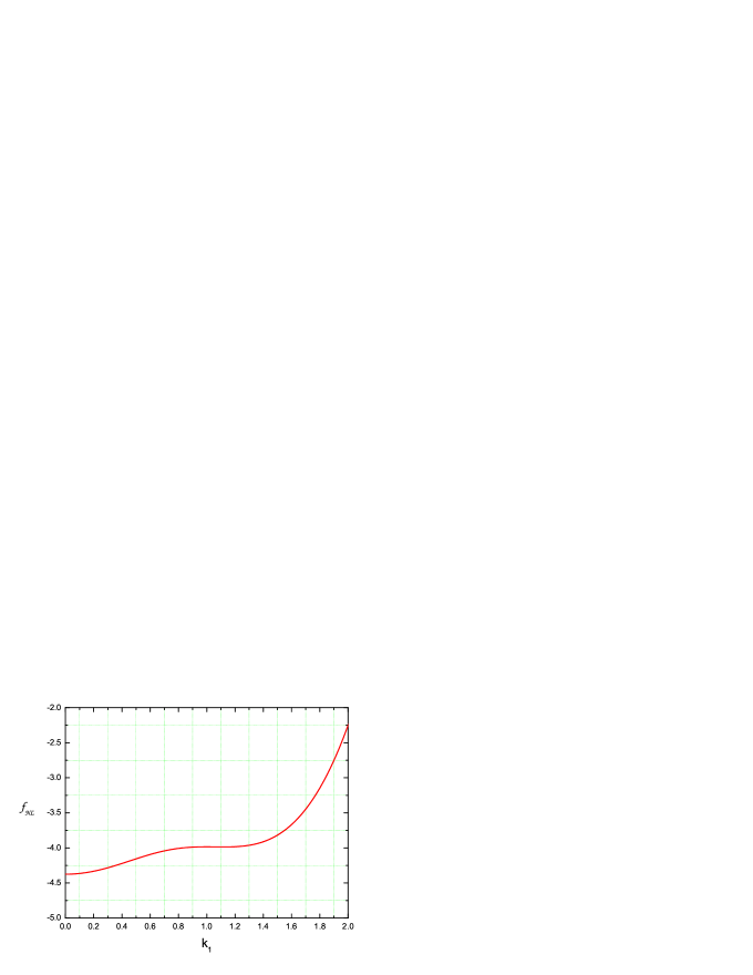
III.4 The Shape of Non-Gaussianity in the Matter Bounce

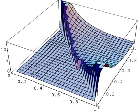
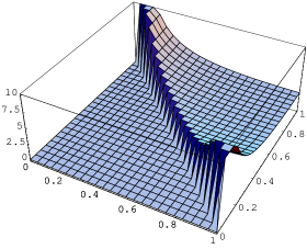
It is interesting to determine the shape of the non-Gaussianities, which has the potential to distinguish different cosmological models once the data will be sufficiently accurate. A useful description of the shape is given by

$$\frac{{\cal A}_{T}}{k_{1}k_{2}k_{3}}~.$$ (42)

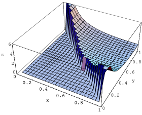
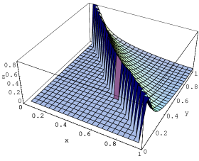
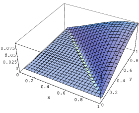
To obtain a better idea of the shape of the non-Gaussianities, we have evaluated Eq. (42) numerically. Our results are plotted in Figures 2), 3), 4) and 5. In the figures, we use the following convention: $k_{3}=1$, the x-axis is $k_{1}$, the y-axis is $k_{2}$, and the z-axis corresponds to the shape ${\cal A}/k_{1}k_{2}k_{3}$. Figures 2), 3) and 4) depict the shape functions of the contributions to order $\epsilon$, $\epsilon^{2}$ and $\epsilon^{3}$, respectively, Figure (5) shows the shape of the total contribution.

Figure 2: The shape of non-Gaussianity in the Matter Bounce. The vertical axis is the negative of the shape function. This figure shows the contribution of the terms of order $\epsilon$.

Figure 3: The shape of non-Gaussianity in the Matter Bounce. This figure shows the contribution of the terms of order $\epsilon^{2}$.

Figure 4: The shape of non-Gaussianity in the Matter Bounce. This figure shows the contribution of the terms of order $\epsilon^{3}$.

Figure 5: The shape of non-Gaussianity in the Matter Bounce. This figure shows the contribution of all terms.

For comparison, the shape function of the non-Gaussianities in single field slow-roll inflation to leading order in the slow-roll parameter $\epsilon$ is shown in Figure 6. We see that the dominant structure of the shape function (modulo sign) is the same in the matter bounce. However, it is also clear that the sub-leading correction terms in the case of the matter bounce shape function are clearly visible. They arise in the terms which are of the order $\epsilon^{2}$ and $\epsilon^{3}$. Therefore, these next-to-leading correction terms in the case of slow-roll inflation are suppressed by orders of magnitude (namely by $\epsilon$) compared to the leading term.

Figure 6: The shape of non-Gaussianity in single field slow-roll inflation to leading order in $\epsilon$. The vertical axis is the amplitude of the shape function.

From the above analysis, we have learned that the amplitude of the non-Gaussianities of metric perturbations predicted in the matter bounce scenario is of order ${\cal O}(1)$, much larger than in single-field slow-roll inflation models. The shape is dominated by a term of local form, but there are sizable corrections with which the matter bounce model could in principle be distinguished from large classes of inflationary scenarios, including many generalized inflation models Chen.

There are two basic reasons leading to these differences. One is that in a bounce model the analog of the slow-roll parameter is large, the other is that the perturbations outside the Hubble radius are not conserved which provides a new origin to generate non-Gaussianities.

III.5 Squeezed Limit

It is also interesting to consider the behavior of shape function in the squeezed limit when $k_{1}=k_{2}\equiv k$ and $k_{3}\rightarrow 0$

In this limit, the leading terms of the above three shape functions for the contributions to orders $\epsilon$, $\epsilon^{2}$ and $\epsilon^{3}$ are all proportional to

$${\cal A}\,\sim\,\frac{k^{5}}{k_{3}^{2}}~\,.$$ (43)

However, when we sum the three contributions, we find that the leading terms cancel and the total shape function takes the form

$${\cal A}_{T}|_{\rm squeezed}\,=\,-\frac{21}{8}k^{3}~.$$ (44)

IV Discussion and Conclusions

We have calculated the amplitude and shape of the non-Gaussianities in the matter bounce model as quantified by the three-point correlation function of $\zeta$. Since in this model the fluctuations grow on super-Hubble scales during the contracting phase, different terms in the interaction Lagrangian dominate the contribution to the non-Gaussianities. In addition, there is no slow-roll suppression of the amplitude. Hence, both the amplitude and the shape are different from what is predicted in inflationary models.

The amplitude of the non-Gaussianity is of the order $O(1)$. Both the amplitude and the sign are fixed, independent of any model parameters, different from the result obtained in the standard paradigm. The amplitude which we predict is smaller than the current upper limits from the WMAP results WMAP, but they are in the range of what the Planck satellite will be able to observe Planck . The shape function contains contributions which are different in shape compared to what is obtained in inflationary models, although the dominant term is of local form. These distinctive contributions arise at order $\epsilon^{2}$ and $\epsilon^{3}$ in the parameter which in the case of single field slow-roll inflation is the slow-roll parameter which is much smaller than $1$, but which in our case is $3/2$. Hence, in our case the extra terms in the shape functions are not suppressed by more than a factor of order unity compared to the contributions which are of similar shape to those which dominate in the inflationary paradigm.

Thus, we conclude that the amplitude and the shape of non-Gaussianities of the three-point function provide distinctive signatures for cosmological models based on a matter bounce. Since the differences in the shape of the non-Gaussianities are mainly due to the growth of the curvature fluctuations on super-Hubble scales in the contracting phase, the shape function of non-Gaussianities in other scenarios in which adiabatic fluctuations are produced in the contracting phase will be similar to what we have obtained here.

Note that we have considered only the case of a canonical kinetic term for the matter fields, and we have focused on the adiabatic mode. Including non-canonical matter fields and entropy modes will give further contributions to the non-Gaussianities which will make the amplitude larger in general, as the inclusion of such effects increases the amplitude of non-Gaussianities in the case of inflation models.

The formalism we have developed here can be used to compute the non-Gaussianities in other collapsing scenarios, for example the Ekpyrotic model KOST. There has been a lot of recent work on non-Gaussian fluctuations in the multi-field variant of the scenario Ekpyrotic. However, the adiabatic mode will also contribute to the non-Gaussianities, and this contribution can be computed easily using our methods.