BayesClumpy: Bayesian Inference with Clumpy Dusty Torus Models

Abstract

Our aim is to present a fast and general Bayesian inference framework based on the synergy between machine learning techniques and standard sampling methods and apply it to infer the physical properties of clumpy dusty torus using infrared photometric high spatial resolution observations of active galactic nuclei. We make use of the Metropolis-Hastings Markov Chain Monte Carlo algorithm for sampling the posterior distribution function. Such distribution results from combining all a-priori knowledge about the parameters of the model and the information introduced by the observations. The main difficulty resides in the fact that the model used to explain the observations is computationally demanding and the sampling is very time consuming. For this reason, we apply a set of artificial neural networks that are used to approximate and interpolate a database of models. As a consequence, models not present in the original database can be computed ensuring continuity. We focus on the application of this solution scheme to the recently developed public database of clumpy dusty torus models. The machine learning scheme used in this paper allows us to generate any model from the database using only a factor $10^{-4}$ of the original size of the database and a factor $10^{-3}$ in computing time. The posterior distribution obtained for each model parameter allows us to investigate how the observations constrain the parameters and which ones remain partially or completely undetermined, providing statistically relevant confidence intervals. As an example, the application to the nuclear region of Centaurus A shows that the optical depth of the clouds, the total number of clouds and the radial extent of the cloud distribution zone are well constrained using only 6 filters. The code is freely available from the authors.

1. Introduction

It is customary that physical information about astrophysical objects cannot be obtained directly from the observables. In such a case, astrophysicists propose a plausible scenario described by a physical model and the procedure is to compare the observables with the predictions of the model with the aim of inferring the physical parameters of the model. The presence of degeneracies (either induced by the presence of noise or intrinsic to the model) introduce complexity in the analysis and they need to be taken into account. This is the subject of Bayesian data analysis that, although it is rooted on ideas developed in the 19th century, it has become practical only in the last decades.

The fundamental idea behind Bayesian data analysis is to take into account that all parameters of a model can be understood as random variables with associated probability distribution functions. The standard problem of model fitting is usually seen as finding the set of model parameters that better reproduce the observables. However, the Bayesian approach is far more informative and transforms the problem into finding the probability distribution function associated with the parameters of the model once the data set is taken into account. In the presence of noise and/or degeneracies, these probability distribution functions represent the complete solution to the problem and automatically include all the statistical information about the parameters that can be inferred from the observables. We have witnessed an enormous interest in Bayesian inference in Astrophysics in the last decade. The reason for this resides in two facts. First, the quality and amount of observed data is usually deficient and one has to rely on methods that exploit to the limit the reduced amount of information. Second, the applied physical models are sometimes too complex as compared with the data available to constrain them. To mention a few recent works, we find applications in cosmological analyses (e.g., Lewis & Bridle, 2002; Rubiño-Martin et al., 2003; Rebolo et al., 2004; Trotta, 2008), gravitational wave analyses (e.g., Cornish & Crowder, 2005), gravitational lensing (e.g., Brewer & Lewis, 2006), oscillation of solar-like stars (e.g., Brewer et al., 2007), analysis of spectropolarimetric data (Asensio Ramos et al., 2007a), analysis of extreme ultraviolet spectral line fluxes (Kashyap & Drake, 1998), and more.

As we review in Appendix A, Bayesian inference techniques can be essentially reduced to the calculation of multi-dimensional integrals (e.g., Neal, 1993; Skilling, 2004; Gregory, 2005; Trotta, 2008). In very simple models, these integrals can be carried out analytically. However, more realistic problems cannot be analytically treated. The explosion of Bayesian analysis methods in the last decades has to be associated with the set of efficient sampling techniques today known as Markov Chain Monte Carlo methods (MCMC; Metropolis et al., 1953; Neal, 1993; Gregory, 2005). In spite of their success, these methods also present the drawback of being computationally intensive because the proposed model has to be evaluated many times. As a consequence, the execution time of these techniques is quite high if the evaluation time of the model is non-negligible. For this reason, there have been some efforts in recent years towards reducing the evaluation time of the models at the expense of a small lost in accuracy. They are based on the development of approximate methods that are able to “learn” a database of models for many combinations of the model parameters. For instance, Fendt & Wandelt (2007) developed a method based on polynomial interpolation for the rapid cosmological parameter estimation problems. Later, Auld et al. (2008) used a neural network approach for the calculation of cosmic microwave background power spectra (only for models in a small hypercube around the commonly accepted region of most probable values for the cosmological parameters) leading to a very fast Bayesian cosmological parameter estimation code.

Our main aim in this paper is to present BayesClumpy, a computer program that allows us to efficiently carry out Bayesian analysis of observed spectral energy distributions coming from the inner region of active galactic nuclei (AGN). To this aim, we use the recently developed clumpy dusty torus model of Nenkova et al. (2008a, b), known as CLUMPY models, and develop a MCMC code whose output is the probability distribution function for all the parameters of the CLUMPY models once the observations are taken into account. As a consequence, the code yields statistically significant estimations of the parameters and, more important, statistically relevant confidence intervals. This facilitates the investigation of degeneracies and can be also used to suggest future observations that can help us introduce stronger constraints in the inference. The code is based on a recently released on-line database of CLUMPY models. We apply an interpolation method like that presented by Auld et al. (2008) that greatly accelerates the evaluation of models. In our case, we manage to make the approximation method work correctly for the whole database and not only for a small hypercube, thus allowing us to efficiently explore the full space of parameters. Finally, the Bayesian character of the approach allows the user to include any a-priori knowledge about any parameter.

2. CLUMPY models

According to the Unified Model for Seyfert galaxies (Antonucci, 1993; Urry & Padovani, 1995), Type-2 AGN are the edge-on counterparts of the face-on Type-1 AGN. This way, in Type-1 AGN the broad-line region (BLR), that is surrounded by a dusty torus of a few parsecs (Tristram et al., 2007), is observed directly, together with the narrow-line region (NLR) emission, whereas in the case of Type-2 AGN, only the NLR emission is seen directly. However, the Unification Model is not universally applicable, since there are several galaxies that do not reveal the broad lines in polarized light.

Regardless, it is clear that there is dust surrounding the central region of AGN distributed in a toroidal shape. The dust grains in the torus absorb the ultraviolet photons from the central engine and, after reprocessing the radiation, are re-emitted in the infrared range. Since many of the predictions of the first compact-torus models (Pier & Krolik, 1992; Granato & Danese, 1994; Efstathiou & Rowan-Robinson, 1995; Granato et al., 1997) have not been confirmed by the observations, the search for a more distributed or complex geometry of the absorbing material around the AGN have been promoted (Nenkova et al., 2002; Fritz et al., 2006; Elitzur & Shlosman, 2006; Ballantyne et al., 2006).

The clumpy dusty torus models (Nenkova et al., 2002, 2008a, 2008b; Hönig et al., 2006; Schartmann et al., 2008) propose that the dust is distributed in clumps, instead of homogeneously filling the torus volume. As an example of the success of these models, they permit to explain, for example, the observed mutations between Type-1 and Type-2 objects detected in the spectra of a few AGN (Aretxaga et al., 1999; Trippe et al., 2008).

Since the reprocessed radiation from the torus is emitted in the infrared, this range is key to put constrains to the clumpy dusty torus models. High-resolution observations at these wavelengths are mandatory, due to the small size of the torus (Tristram et al., 2007). This way, it is possible to separate the nuclear emission from that of the surrounding galaxy. Important observational constraints for the torus models come then from the shape of the infrared spectral energy distributions (SEDs). Accuracy in the photometry, a filter set spanning a broad wavelength range, and well-sampled SEDs are required to restrict the model parameters.

The CLUMPY models that we use in this work (described in Nenkova et al., 2008a, b) consist of a clumpy distribution of matter with a radial extent characterized by $Y=R_{\mathrm{o}}/R_{\mathrm{d}}$, that is the ratio of the outer to the inner radii of the toroidal distribution. The inner radius ($R_{\mathrm{d}}$) is defined by the dust sublimation temperature. Each clump is specified by its optical depth ($\tau_{V}$), and all clumps are assumed to have the same optical depth. The dust extinction profile corresponds to a standard cold/oxygen-rich ISM dust (Ossenkopf et al., 1992). These clumps, of a given dust composition, are heated by an AGN with a given spectral shape and luminosity. Thus, the inner radius ($R_{\mathrm{d}}$) is determined uniquely by the luminosity and the chosen dust sublimation temperature. The number of clouds along a radial equatorial path is defined as $N$. The radial density profile is a power law ($r^{-q}$), with an angular distribution characterized by a width parameter, $\sigma$.

Figure 1.— First 16 PCA eigenvectors obtained from the CLUMPY database. We have demonstrated that the full CLUMPY database can be decomposed using only the first 13 eigenvectors with great precision. The wavelength variation of the standard deviation of the difference between the original models and the truncated reconstruction is shown in Fig. 3.

3. BayesClumpy

Every CLUMPY model requires several seconds to be calculated. For the typical lengths of converged Markov Chains, this would amount to something between 1 and 6 days per Markov Chain for only one run of the inference problem. Obviously, this is something that is absolutely unacceptable if one wants to carry out inference for many AGN.

The computational efforts carried out by the CLUMPY group has allowed them to calculate and distribute for public access around 2$\times$10⁵ models (now increasing to more than 10⁶ models). They have been calculated for a quite fine grid of model parameters. This database can be used to overcome the difficulty of evaluating the CLUMPY models by using it for interpolation. The reason for interpolation is that the MCMC code will propose models that are not present in the original grid, so that an efficient interpolation method has to be applied. If the interpolation method is fast enough, it will allows us to carry out systematic studies of the compatibility of model parameters with different observations in a completely Bayesian framework. Studies like analyzing the amount of information added by a given filter and which parameters can be confidently recovered from the data are possible under this framework.

In the following sections we describe our approach for interpolation. It is based on the application of two different machine learning techniques: principal component analysis (PCA) for dimensionality reduction and artificial neural networks (ANN) for the interpolation. Such a method has been already applied by Auld et al. (2008) for approximate Bayesian inference of cosmological parameter in a small hypercube around the commonly accepted values of the cosmological parameters. A similar approach has also been employed by Carroll et al. (2008) for the fast synthesis of Stokes profiles in magnetic atmospheres and the quick solution of Zeeman-Doppler imaging problems.

3.1. Principal Component Analysis

Each SED in the database is sampled at $N_{\lambda}=124$ wavelength points. Clearly, some correlations exist between different wavelength points, so that when the flux at a given wavelength is modified, the surrounding wavelength points are also modified in a very similar way (continuity of the SED). As a consequence, the dimension of the non-linear manifold in which the SEDs “live” is much smaller than 124 (see Asensio Ramos et al., 2007b). This fact can be harnessed to apply dimensionality reduction techniques and efficiently compress the database. Although many complex technique exist, we apply here a very basic linear dimensionality reduction technique based on the Principal Component Analysis (PCA; see Loève, 1955) also known as Karhunen-Loève transformation. Briefly, the idea is to obtain a self-consistent basis (principal components) in which the data can be efficiently developed. This basis has the property that the largest amount of variance is explained with the least number of basis functions. It is useful to reduce the dimensionality of data sets because most part of the variability of the signal is carried by the first $N^{\prime}\ll N_{\lambda}$ eigenvectors. Note that, since PCA performs a linear analysis, it is not possible to reduce the dimensionality of the transformed manifold to the real dimensionality of the non-linear manifold and the number of necessary eigenvectors is larger than the number of physical parameters of the model (Asensio Ramos et al., 2007b). See appendix B for more technical details on PCA.

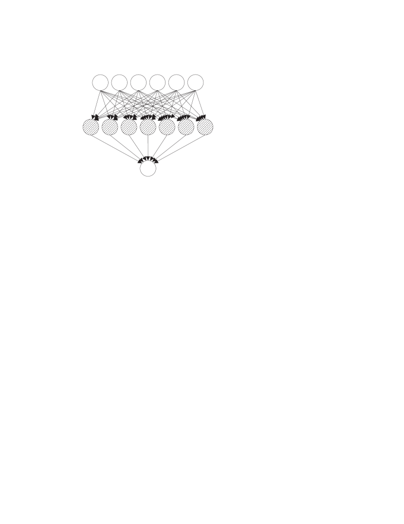
Figure 2.— Topology of the artificial neural networks applied in this work. The neural networks contain an input layer of six neurons for the six fundamental parameters of the CLUMPY models. The output layer is composed of only one neuron that is associated with the projection of the SED along each PCA eigenvector. The intermediate layer (widely known as “hidden” layer) is used to obtain the non-linear mapping between the input and the output layers.

The first 16 PCA eigenvectors obtained from the CLUMPY database are shown in Fig. 1. This figure shows that low-order eigenvectors are very smooth and take into account large-scale variations that are seen in the majority of the SEDs. On the contrary, high-order eigenvectors contain high-frequency details that produce small-scale details in a small amount of SEDs. Choosing only the first $N^{\prime}=13$ eigenvectors results in a very good representation of the whole database. In other words, this allows us to reduce the size of the database because we only need to give 13 numbers for each SED (the projection of each SED along each PCA eigenvector) and their associated eigenvectors. Note that, for very large number of models $>10^{5}$, the reduction in size of the database tends to $13/N_{\lambda}$, which is close to 1/10 in our case.

Although the PCA eigenvectors can be usually associated to different physical mechanisms (e.g., Skumanich & López Ariste, 2002), our aim here is not to analyze them. We treat the PCA eigenvectors as a basis set of purely mathematical character that allows us to efficiently develop the database. Efficiency in our case means that the number of eigenvectors needed to reproduce the database with a given error bar is the smallest possible. In any case, it is possible to see some well-known signatures like the 10 µm one produced by dust emission/absorption in some eigenvectors of Fig. 1.

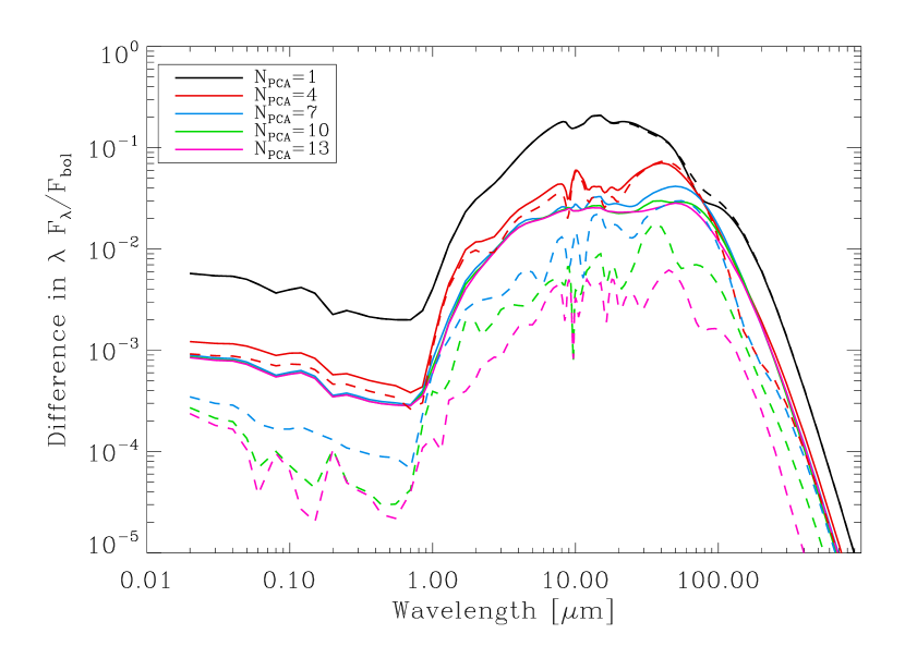
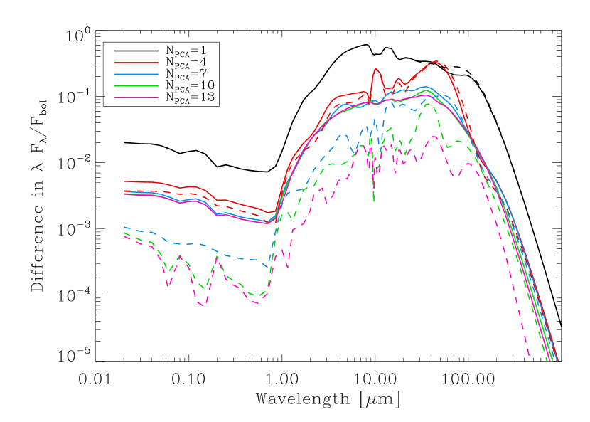
Figure 3.— Reconstruction errors characterized by the standard deviation (left panel) and 99% percentile (right panel) of the difference in $\lambda F_{\lambda}/F_{\mathrm{bol}}$ between all the SEDs of the original database and the reconstructed SEDs using an increasing number of PCA eigenvectors for the reconstruction. The quantity $F_{\mathrm{bol}}$ is the bolometric luminosity of the AGN. The dashed lines show the results obtained when the PCA coefficient of each SED is obtained using the exact SED for projecting along each eigenvector. The solid line corresponds to the results obtained when the ANN is used to obtain the projection along each PCA eigenvector. Note that the quality of the reconstruction depends on wavelength due to the existence of variable features in some spectral ranges.

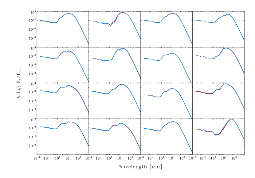
Figure 4.— Example of the interpolation obtained with the ANN approach. The black lines are the SEDs corresponding to randomly chosen physical parameters. The red lines are those reconstructed using the first 13 PCA eigenvectors using the projection of the exact SED on each PCA eigenvector. The blue lines are the results obtained using the ANN-based reconstruction. Note that the real SEDs are not seen because the rest of curves overlap.

3.2. Neural Network

Although the PCA dimensionality reduction step has reduced the size of the database, it is still complex and time consuming to obtain the SED for values of the parameters not present in the original grid. For this reason, we have developed an interpolation method based on an artificial feed-forward neural network (ANN; see e.g., Neal, 1993), a widespread machine learning technique that usually presents very good behavior. We have developed $N^{\prime}$ simple neural networks whose topology is shown in Fig. 2. The ANN consists of an input layer formed by 6 neurons that accept the physical parameters of the CLUMPY models. The output layer is formed by one neuron whose value is the projection of the SED corresponding to the physical parameters of the input layer along each PCA eigenvector calculated before. Both layers are fully connected by an intermediate hidden layer. The approximation properties of three-layered neural networks is something known after the universal approximation theorem (e.g., Cybenko, 1988; Neal, 1993). This theorem states that such a neural network, with a sufficiently large number of neurons in the hidden layer, can approximate any continuous function. We have verified that, in order to get a compromise between the approximation abilities of the neural network and the speed of evaluation, values of $N_{h}$ between 30 and 50 give very good results. This method is not optimal because the values of $N_{h}$ are set empirically. More refined methods probably based on Bayesian model selection (or the approximate minimum description length method used by Asensio Ramos, 2006) can be used to infer the optimal number of hidden neurons based on objective measurements. However, for the purpose of our work, the employed method is enough to ensure good approximation properties while maintaining a fast execution speed. The ANN uses the hyperbolic tangent activation function. Prior to utilizing the neural network, all the input and output values are normalized to the interval $[-1,1]$ to improve the interpolation abilities of the network.

The training of the ANN is done by modifying the weights until the minimizing the quadratic difference between the output of the neural network and the correct values of the database (see appendix C for more details). It is important to note that over-fitting has been avoided using two data-sets chosen randomly from the database: one for training and one for validation purposes. The training process is stopped when the quadratic error decreases for the training set but starts to increase for the validation set. We have verified that it is possible to carry out the training of the neural networks using only a subset of the full database, which greatly accelerates the process. This is a consequence of the smooth variation of the SEDs with the physical parameters. Picking randomly from the database a training set with $\sim 10$% of the total number of models, the trained neural network does a very good job with the validation set and with the whole database.

In order to analyze the ability of the PCA+ANN combination to reproduce the database, we show in Fig. 3 the standard deviation (left panel) and the 99% percentile (right panel) of the distribution of differences in $\lambda F_{\lambda}/F_{\mathrm{bol}}$ between the exact SEDs of the full database and the reconstructed SEDs. The 99% percentile has been also represented in order to test the possibly poor generalization properties of neural networks in regions close to the boundaries of the space of parameters. The dashed lines present the results when the PCA reconstruction is done using the original database. In such a case, the reconstruction error is monotonically decreasing with the number of included PCA eigenvectors. If all the eigenvectors are used, the reconstruction error turns out to be identically zero. With the first 13 eigenvectors, the reconstruction errors are below 5$\times$10^-3 ($1\sigma$) and 10^-2 (99 % percentile) in all the wavelength range of interest. The solid lines are the reconstruction errors when the projections along the PCA eigenvectors are calculated by evaluating the artificial neural networks. Obviously, due to the approximate character of the neural networks’ interpolation, the reconstruction errors are larger than in the exact case. The approximation abilities of the neural networks worsen when the order of the eigenvector increases. The reason is that these eigenvectors contain high-frequency or less abundant signatures whose variation with the parameters are less smooth. However, standard deviations of the reconstruction error are below 2$\times$10^-2 in the whole spectral domain of interest, with errors going down to 10^-3 in some spectral windows. Concerning the 99% percentile, errors are always below 10^-1, with wavelength regions close to 10^-3.

An example of the ability of the ANN to approximate the database is shown in Fig. 4, where the black line is the exact SED obtained from the database (note that although only part of the database was used in the training, these SEDs are obtained randomly from the full database). The red line is the SED reconstructed using only the first 13 eigenvectors but using the correct SED for the projections along the eigenvectors. The blue line is the SED reconstructed using the neural networks. Note that differences are hardly noticeable and are well below any possible observational error or indeterminacy in the physical properties of the AGN.

Table 1Centaurus A high spatial resolution nuclear density measurements from Meisenheimer et al. (2007) and Radomski et al. (2008).

Filter	Central wavelength (µm)	Flux Density (mJy)
NACO J	1.28	1.3$\pm$0.1
NACO H	1.67	4.5$\pm$0.3
NACO Ks	2.15	33.7$\pm$2.0
NACO L’	3.80	200$\pm$40
T-ReCS Si2	8.74	710$\pm$40
T-ReCS Qa	18.3	2630$\pm$650

3.3. Advantages

There are two main advantages of the approach followed in this paper. On the one hand, it opens the possibility to interpolate in the database, so that it is now possible to calculate SEDs for combinations of parameters that were not present in the original grid. In principle, if the SEDs depend smoothly on the parameters, the neural networks should have captured all the variability and there is no necessity to improve the griding of the original database. On the other hand, the synthesis of the SED is extremely simple and fast because all the details of the calculations inherent to the CLUMPY model are approximated by the neural networks. One has to calculate the 13 projections of the SED onto the PCA eigenvectors by evaluating the 13 neural networks given by Eq. (C3). Then, the reconstruction of the SED is obtained by adding the first 13 PCA eigenvectors weighted by these 13 projections. In terms of computational time, this makes it possible to synthesize $\sim 10^{4}$ SEDs in just a minute, so that we obtain a gain in time of a factor 10³ or larger. The ANN+PCA approach can be essentially considered as a huge compression of the database. Instead of saving the whole database, one only needs to save the weights of the neural networks and the PCA eigenvectors. In our case, the complete database amounts to $\sim$430 Mb, while the ANN+PCA approach amounts to $\sim$40 kb, with a reduction factor that is close to 10⁴, with the added benefit of being able to easily interpolate. Of course, this improvement in the calculation speed is compensated by small differences as compared with the correct SEDs.

3.4. Simulating filter photometry

For the cases in which the observations are of filter photometry kind, once the SED is obtained with the previous formalism, it remains to simulate the effect of the filters on the simulated SED. Given that $\phi(\lambda)$ is a filter normalized to unit area used to obtain a point in the observations, the synthetic value is obtained by just evaluating:

$$f(\lambda_{c})=\int_{-\infty}^{\infty}F(\lambda)\phi(\lambda)\mathrm{d}\lambda,$$ (1)

where $\lambda_{c}$ is the central wavelength of the filter, obtained as:

$$\lambda_{c}=\int_{-\infty}^{\infty}\lambda\phi(\lambda)\mathrm{d}\lambda.$$ (2)

Both integrals are approximated in BayesClumpy with a very simple trapezoidal quadrature:

$$\tilde{f}(\lambda_{c})=\sum_{i}w_{i}F(\lambda_{i})\phi(\lambda_{i}),$$ (3)

with $w_{i}$ the weights of the trapezoidal quadrature.

4. Illustrative example

We have implemented this forward modeling code into a Markov Chain Monte Carlo sampling algorithm that is used to evaluate the posterior distribution function for the physical parameters once an observation is provided (see appendix A for details). The filters at which the information is available are fully configurable from a database of filters belonging to different instruments. One only needs to select the filter and give the the observed flux, $d_{i}$, and its corresponding error. For the moment, Gaussian errors with standard deviation $\sigma_{i}$ and upper limits within a certain (user-selectable) confidence level are possible.

The simplest version of the code uses uniform priors for all the parameters and admit to give the upper and lower limits for every parameter. It is also possible to choose a Gaussian prior in case any parameter is known a-priori to be around a given value with a certain dispersion. The central position and the width of the Gaussian are the only adjustable hyper-parameters in this case. More complex prior distributions are straightforward to include in the code and can be fully configurable.

Apart from the 6-dimensional vector of parameters of the CLUMPY model given by $(\sigma,Y,N,q,\tau_{V},i)$, we add other parameters like a vertical shift in logarithmic scale that accounts for the normalization in luminosity of the SED or the amount of interstellar extinction characterized by an extinction law and the absorption at visible wavelengths. We neglect the presence of extinction in this work, but the effect of the normalization in luminosity is treated as a nuisance parameter and all the results are presented with this parameter integrated out (marginalized). Since the marginal posterior distributions of the vertical shift are already an output of BayesClumpy, one can carry out inference over the total luminosity of the AGN.

4.1. Observations

High resolution infrared data have been compiled from the literature for the Seyfert 2 galaxy Centaurus A (NGC 5128) in order to construct a purely-nuclear SED. Centaurus A is the closest active galaxy, with its core heavily obscured by a dust lane, and consequently only visible at wavelengths longwards of 0.8 µm (Schreier et al., 1998; Marconi et al., 2000).

Figure 5.— Marginal posterior distributions for all the free parameters of the CLUMPY model considered here. Note that $\tau_{V}$ and $N$ are nicely constrained. Other distributions only favor certain values of the space of parameters. The vertical shift of the SED, treated as a nuisance parameter, has been marginalized.

Near-infrared data obtained with Naos-Conica (NACO) at UT4 have been compiled from Meisenheimer et al. (2007). Conica is a high spatial resolution near-infrared imager and spectrograph (Lenzen et al., 1998), that works together with Naos, the Nasmyth Adaptive Optics System (Rousset et al., 1998), providing adaptive-optics corrected observations in the range 1-5 µm. Meisenheimer et al. (2007) found the nucleus unresolved at all wavelengths with a FWHM of 0.10″ in the J band, 0.088″ in the H band, 0.059″ in the Ks band, and 0.090″in the L’ band. The fluxes corresponding to this unresolved component have been compiled and reported in Table 1.

High spatial resolution mid-infrared data of the nucleus of Centaurus A are also compiled from Radomski et al. (2008). The observations were taken in the Si2 filter (8.8 µm) and in the Qa band (18.3 µm) using the mid-infrared imager/spectrometer T-ReCS on Gemini South (Telesco et al., 1998). The core is also unresolved in this range, surrounded by a diffuse extended emission. In these bands, the upper limits to the size of the unresolved nucleus are 0.19″ at 8.8 µm and 0.21″ at 18.3 µm at the FWHM level.

With these high spatial resolution density measurements of the unresolved component of Centaurus A, we can construct a purely-nuclear SED of this galaxy, to be fitted with the CLUMPY models, as an example of the use of our tool.

4.2. Bayesian Analysis

The parameter estimation results presented in this section have been carried out with a Markov Chain of length $6\times 10^{5}$, of which we take out the initial 40% as a burn-in (transitory initial portion of the Markov Chain in which the algorithm is not correctly sampling the distribution; see, e.g., Neal, 1993; Gregory, 2005). Our experiments have shown that the transitory phase is quite short and that the burn-in can be safely reduced to just the first $\sim 10$% of the chain without much problem, thus increasing the quality of the sampling. Although a 40% burn-in is surely excessive, the fact that the MCMC scheme works very fast (less than half a minute for a $6\times 10^{5}$ chain), we prefer to run a longer chain and maintain the large burn-in. This way we make sure that the MCMC algorithm is well mixed and we are sampling correctly the posterior distribution.

The one-dimensional marginalized posterior distributions are shown in Fig. 5 for all the free model parameters. These distributions are obtained as histograms of the Markov Chain for each parameter due to the automatic marginalization properties of the MCMC technique. This information encodes, for every parameter, the effect of ambiguities and degeneracies (the marginalization of the posterior takes into account all the possible values of the rest of parameters weighted by their probabilities) and summarizes the statistical properties of the estimation for each parameter. Uniform priors have been employed, leaving for a later publication the analysis of AGN in which a-priori knowledge might be present (Ramos Almeida et al., 2009, in preparation). Therefore, these posterior distributions have to be compared with uniform distributions giving equal probability to all combinations of parameters. When the observed data introduces enough information into the problem, the posterior distributions clearly differ from the uniform distribution. The uniform distributions are truncated to the following intervals: $\sigma=[15,75]$, $Y=[5,30]$, $N=[1,15]$, $q=[0,3]$, $\tau_{V}=[10,60]$ and $i=[0,90]$. These values are based on physically reasonable assumptions that avoid non-realistic solutions.

Figure 5 clearly indicates that all the parameters are nicely constrained for Centaurus A. The marginal distribution of $\tau_{V}$, with its asymmetric shape, is showing us that the observations are able to put an upper limit to its value. The calculation of the confidence intervals in this histogram gives us that the upper limit to $\tau_{V}$ is 11.2 at 68% ($1\sigma$ level) confidence and 13.0 at 95% confidence ($2\sigma$ level). Concerning $N$, there is a tail towards large values that produce slightly asymmetric error bars. If we summarize the histogram using the median, we find that $N=3.1^{+0.7}_{-0.5}$ at 68% confidence and $N=3.1^{+2.0}_{-0.9}$ at 95% confidence. It is also possible to use different quantities to summarize the statistical information, like the posterior mean or the posterior mode (maximum-a-posteriori or MAP), although the relevant information is provided by the full marginal posterior distribution.

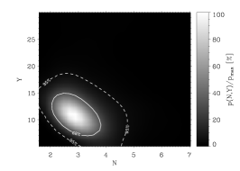
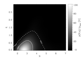
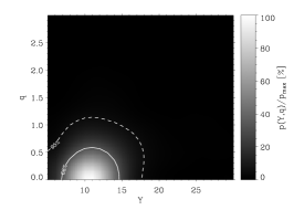
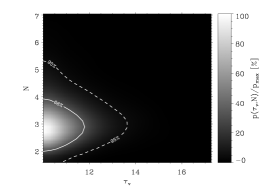
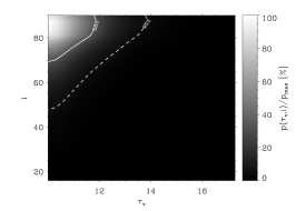
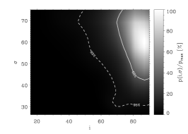
Figure 6.— Two-dimensional marginal posterior distributions (joint distribution) for several combinations of parameters. The contours indicate confidence regions at 68% and 95%.

The marginal posterior for $Y$ also indicates that it is a nicely constrained parameter, again with asymmetric error bars due to the enhanced tail. We obtain $Y=11.5^{+2.9}_{-2.3}$ at 68% confidence and $Y=11.5^{+8.6}_{-4.3}$ at 95% confidence. A different behavior is found for $\sigma$, $q$ and $i$. In the three cases, there is a region of the space of parameters that is favored with respect to others. For instance, the Bayesian analysis gives a larger probability to inclinations close to 90^∘ (the MAP value is $\sim 90^{\circ}$), practically discarding angles close to 0^∘. The same happens for $q$, in which data favor values close to zero. Summarizing, we get $i>78^{\circ}$, $\sigma>56^{\circ}$ and $q<0.47$ with 68% confidence.

Correlations between the parameters can be understood at the light of the two-dimensional marginal distributions of Fig. 6, where the contours mark the 68% and 95% confidence regions. Instead of plotting all possible combinations of parameters, we only show six cases that are representative of the general behavior. It can be seen that the observed data discard large values of $N$, $Y$, $\tau_{V}$ and $q$. The plot $\sigma-i$ presents weakly constrained parameters, although it is clear from this figure that large values of $i$ are favored (in accordance with the Type-2 classification of Cen A). Small values of $i$ are not preferred and become slightly more likely as $\sigma$ increases (i.e., as the probability that the central engine is blocked from view). In other words, the results show that Type-1 orientations (small $i$ simultaneous with small $\sigma$) are not favored by the data. We present the physical interpretation of these results in Ramos Almeida et al. (2009, in preparation).

It turns out interesting that there is not much ambiguity in the parameters so that the available data is able to constrain the large variability of the clumpy torus models. One should expect to obtain even more constrained marginal posterior distributions when increasing the number of filters.

Although the solution to the Bayesian inference problem are the posterior distributions shown in Fig. 5, one can try to represent the models corresponding to the median or the maximum-a-posteriori values of the parameters (within the confidence intervals) to visually compare them with the observations. The maximum-a-posteriori model is displayed in solid line in Fig. 7. This is obtained using the combinations of parameters that maximize the posterior distribution. The dashed line shows the model obtained using the medians of the marginal posterior distribution for each parameter. Finally, the dashed line tries to give an idea of the range of variability of the compatible models. It is built by synthesizing SEDs for all combinations of parameters taking into account their confidence intervals around the median value.

5. Conclusions

This paper presents a computer code for the Bayesian analysis of nuclear SEDs of AGN using CLUMPY models. This approach allows us to obtain the full solution to the inference problem in terms of posterior probability distributions of the model parameters. These probability distributions take into account the a-priori information about the parameters and the information introduced by the observations. Presently, the prior distribution can be selected to be uniform in an interval, Gaussian or Dirac delta. According to the observations, the code admits observations corrupted with Gaussian noise and/or upper limit detections.

The machine learning technique based on the combination of the PCA decomposition and the application of artificial neural networks for the approximation of the database leads to a gain of a factor $10^{4}$ in disk storage and $10^{3}$ in execution time. As a sub-product, it provides the possibility to interpolate in the database, thus it becomes feasible to generate SEDs for combinations of parameters not present in the original grid. This characteristic will be of great importance for the analysis of the response function of the SED in certain spectral ranges of interest to the model parameters (derivatives of the SED with respect to the model parameters).

Figure 7.— High-resolution nuclear SED of Centaurus A, constructed with near- and mid-infrared data shown in Table 1. The solid line presents the maximum-a-posteriori estimation of the SED while the dashed line is the one calculated with the median of the marginal posterior distributions of the parameters. The shaded region is the range of SEDs compatible within the 68% confidence interval for each parameter.

Although the space of parameters is very large, the approximation properties of the method are very good, giving differences between the exact and the approximate SED with a standard deviation below 0.1 dex in the spectral window of interest. These errors are clearly below any uncertainty in the observations, so that the final results will not be dominated by the approximation step. This good behavior is possible because of two reasons. First, the variation of the SEDs is notably smooth when the physical parameters are varied. This greatly facilitates the interpolation properties of the artificial neural networks. Second, the precision needed in the approximation is not specially significant and one only needs to train the neural networks until the differences between the exact SEDs and the reconstructed SEDs are below the observational errors.

In order to demonstrate the output of the code, we have shown an example with Centaurus A. The analysis of the marginal posterior distributions shows that some parameters are nicely determined by the data, while other parameters remain less constrained. Although one can summarize the marginal posteriors using modes, medians and/or means, together with confidence intervals, the true solution to the problem from the Bayesian point of view are the histograms shown in Fig. 5.

Although BayesClumpy is focused towards the analysis of nuclear SEDs of AGN using CLUMPY models, the core of the method remains completely general and can be applied to a myriad of problems for which one is interested in fitting an already built database of models to observations. Cases like the database of synthetic spectra computed for the GAIA project (e.g., Brott & Hauschildt, 2005) or the analysis of the spectral energy distributions of protostars (e.g., Robitaille et al., 2007) are examples of potential applications. Apart from the gain in speed in the analysis, one would be able to carry out a fully Bayesian analysis of the observations, thus opening the possibility of including prior information and/or carrying out marginalization of nuisance parameters. Furthermore, Bayesian model selection techniques would facilitate the objective selection of several competing models for explaining the observables.

BayesClumpy is coded in Fortran 90 with a graphical front-end developed in IDL. We offer BayesClumpy to the astrophysical community with the hope that it will help researchers to take advantage of the CLUMPY models for analyzing observed SEDs. To get a copy, it suffices with making an e-mail request to the authors of this paper.

Appendix A Bayesian Inference

A.1. Fundamental considerations

BayesClumpy is a computer code that is focused towards analyzing observed SEDs using theoretical models and carrying out inference over the parameters of the theoretical models. It is built under the framework of the Bayesian approach for the inference (see e.g., Neal, 1993; Gregory, 2005), of which we briefly summarize the main ideas. Let $M$ be a model that is proposed to explain an observed data set $D$. In our case, $D$ is usually the set of points observed using filter photometry, but more information can be introduced if the observation is of spectroscopic type. Additionally, $M$ is the CLUMPY model described by Nenkova et al. (2008a, b) that we have briefly described in §2. Let $I$ be a set of sensible background a-priori knowledge about the problem (for instance, the filters used for the observations). In general, the model $M$ is described by a set of equations or algorithms that depend on a vector of parameters, $\theta$. These parameters usually have a physical meaning and our aim is to obtain information about these parameters from the observations. Inside the Bayesian framework for inference, our approach is the one of parameter estimation. In the case at hand, the vector of parameters contains the six free parameters of the CLUMPY model already described in §2.

In general, due to the presence of noise in the observations, any inversion procedure is not complete by just giving the values of the model parameters that better fit the observations. The full inference problem has to provide the posterior probability distribution function (PDF) $p(\mbox{\boldmath$\theta$}|D,I)$ that describe the probability that a given set of parameters $\theta$ is compatible with the observables $D$ given the set of background a-priori assumptions $I$. As a consequence, statistically relevant information can be obtained from this PDF by marginalization (integration) of unimportant parameters. Specifically, the marginalization of all the parameters except the one in which we are interested will give the probability distribution function of the parameter taking into account all possible compatible values of the rest of parameters. Therefore, ambiguities and degeneracies in the parameters are translated into marginal posterior distributions with heavy tails. The cornerstone of the Bayesian approach to inference is the Bayes theorem, that relates the posterior distribution $p(\mbox{\boldmath$\theta$}|D,I)$ with any a-priori knowledge and the information introduced by the data:

$$p(\mbox{\boldmath$\theta$}|D,I)=\frac{p(D|\mbox{\boldmath$\theta$},I)p(\mbox{\boldmath$\theta$}|I)}{p(D|I)},$$ (A1)

where $p(D|I)$ is the so-called evidence, $p(\mbox{\boldmath$\theta$}|I)$ is denominated the prior distribution and $p(D|\mbox{\boldmath$\theta$},I)$ is the so-called likelihood.

The evidence, equal to the integral of the posterior distribution over the parameter space, plays no role in the context of parameter estimation because it is a constant that does not depend on the model parameters $\theta$. However, it turns out to be crucial in the context of model selection. Strictly speaking, when one carries out parameter estimation in the Bayesian context, one should indicate the estimation of the parameters, the error bars and the value of the evidence. This way, other researchers can compare their results with already published ones. The main difficulty is that the evidence is very difficult to calculate and specifically designed algorithms are needed (Skilling, 2004; Gregory, 2005).

The prior distribution, $p(\mbox{\boldmath$\theta$}|I)$, contains all relevant a-priori information about the parameters of the model. Usually, unless some information is available about the value of some parameters, it is common to use uninformative priors like bounded uniform distributions or Jeffreys’ priors (e.g., Gregory, 2005). In case our a-priori knowledge of a parameter is sufficient to better constrain the value of a parameter, the Bayesian approach can easily introduce the information into the inference process by appropriately setting the prior distribution $p(\mbox{\boldmath$\theta$}|I)$. Among the options, one can select exponential distributions if large values of the parameters are less probable, Gaussian distributions around a given value with a certain width if there is a region of the space of parameters with more probability, etc.

Finally, the likelihood $p(D|\mbox{\boldmath$\theta$},I)$ is a distribution that gives the probability that the observed data set has been obtained using the set of parameters $\theta$. Assuming that the observables are represented by the vector $\mathbf{d}$ of length $N$ and that the model $M$ evaluates to the vector $\mathbf{y}$ of the same length contaminated by a noise component $\mathbf{e}$, we can write:

$$y_{i}=d_{i}+e_{i},\qquad\forall i.$$ (A2)

When the chosen model parameters exactly correspond to those of the observed data set, the distribution of differences $y_{i}-d_{i}$ has to follow the distribution of the noise. Assuming that the noise is Gaussian distributed with a variance described by the vector $\mbox{\boldmath$\sigma$}^{2}$, the likelihood function is given by:

$$p(D|\mbox{\boldmath$\theta$},I)\propto\prod_{i=1}^{N}\exp\left[\frac{(y_{i}-d_{i})^{2}}{\sigma_{i}^{2}}\right],$$ (A3)

although other distributions can be used. For instance, in cases where only the upper of lower limit is known with a given confidence, it is possible to use skewed likelihood functions that appropriately take this into account. For simplicity, we assume one-sided Gaussian likelihoods centered at zero in which $\sigma_{i}$ is adjusted so that the ratio of the integral of the likelihood between 0 and $d_{i}$ and its total area equals the confidence level of the observation.

Summarizing, Eq. (A1) states that the probability that a model $M$ becomes plausible after the data $D$ has been taken into account (posterior) depends on how plausible the model was before presenting the data (prior) and how well the model fits the data (likelihood).

A.2. Technicalities: the Markov Chain Monte Carlo method

In order to calculate the posterior probability distribution function for one parameter and give estimations and confidence intervals, we have to marginalize (integrate out) the rest of parameters from the full posterior distribution:

$$p(\theta_{i}|D,I)=\int\mathrm{d}\theta_{1}\mathrm{d}\theta_{2}\cdots\mathrm{d}\theta_{i-1}\mathrm{d}\theta_{i+1}\cdots\mathrm{d}\theta_{N_{\mathrm{par}}}p(\mbox{\boldmath$\theta$}|D,I).$$ (A4)

To this end, BayesClumpy utilizes a Markov Chain Monte Carlo (MCMC; Metropolis et al., 1953; Neal, 1993; Gregory, 2005) scheme based on the Metropolis algorithm. The output of the MCMC method is a chain of models whose probability distribution follows the posterior distribution function. The MCMC technique can be also considered as an integration method that returns marginal probability distribution for each parameter in the model. As a consequence, the converged final Markov Chain obtained for each parameter automatically gives, after making histograms, its marginal posterior distribution (integrating out the rest of model parameters). Technically, our MCMC method works by proposing models using a multivariate Gaussian proposal distribution and accepting or rejecting the proposed models based on a standard Metropolis acceptance rule. The proposal density distribution used in the first steps of the chain is a multivariate Gaussian with diagonal covariance matrix that is set to 10% of the allowed range of variation of the parameters. After a configurable initial period, the proposal density is changed to a multivariate Gaussian with a covariance matrix that is estimated from the previous steps of the chain. In order to improve convergence, the covariance matrix is modified by a parameter that assures that the acceptance rate of proposed models is close to 25%, a value that is close to the theoretical optimal value for simple problems (Gelman et al., 1996).

Although MCMC methods represent a huge step forward in the practical application of Bayesian methods to the inference, one of the most important drawbacks is the necessity to sample the whole posterior probability distribution, something that can be very time consuming. Typical MCMC runs require Markov Chains of the order of 10⁴-10⁵ steps in order to end up with correctly converged chains. In case the evaluation of the forward model is not negligible, the total time can be quite large and the systematic analysis of different observations remains completely unpractical.

Appendix B Principal Component Analysis

Let us define $\mathbf{O}$ as the $N_{\mathrm{models}}\times N_{\lambda}$ matrix containing the wavelength variation of all the theoretical SEDs of the database where the mean SED has been substracted. The principal components can be found as the eigenvectors of this matrix of observations, so that they can be obtained by just diagonalizing the matrix $\mathbf{O}$. Since we have $N_{\mathrm{models}}\gg N_{\lambda}$, this matrix is not square by definition and the dimension of the matrix can be so large that computational problems can arise. However, it can be demonstrated that the right singular vectors of the matrix $\mathbf{O}$ are equal to the singular vectors of the covariance matrix:

$$\mathbf{X}=\mathbf{O}^{\dagger}\ \mathbf{O},$$ (B1)

that can be calculating with the Singular Value Decomposition algorithm (SVD; see, e.g., Press et al., 1986). The matrix $\mathbf{X}$ is the $N_{\lambda}\times N_{\lambda}$ covariance matrix and the superindex ${\dagger}$ represents the transposition operator. The same applies to the left singular vectors, which are also eigenvectors of the covariance matrix $\mathbf{X}^{\prime}=\mathbf{O}\ \mathbf{O}^{\dagger}$. The matrix $\mathbf{X}^{\prime}$ has dimensions $N_{\mathrm{models}}\times N_{\mathrm{models}}$ and is typically much larger than the matrix $\mathbf{X}$. However, both descriptions are completely equivalent. The $i$-th principal components, $\vec{b}_{i}$, fulfills:

$$\mathbf{X}\vec{b}_{i}=k_{i}\vec{b}_{i},$$ (B2)

with $k_{i}$ its associated eigenvalue. Writing all the eigenvectors as column vectors in the unitary matrix $\mathbf{B}$ of dimensions $N_{\lambda}\times N_{\lambda}$, since this represents a complete basis of the database, the observations can be written as a linear combination of them as follows:

$$\mathbf{O}=\mathbf{C}\ \mathbf{B}^{\dagger},$$ (B3)

being $\mathbf{C}$ the $N_{\mathrm{models}}\times N_{\lambda}$ matrix of coefficients, whose $C_{ij}$ element represents the projection of the observation $i$ on the eigenvector $j$:

$$\mathbf{C}=\mathbf{O}\ \mathbf{B}.$$ (B4)

The dimensionality reduction is carried out by using the matrix $\mathbf{\hat{B}}$ that contains only the first $N_{\mathrm{red}}$ eigenvectors that have been retained as containing the majority of signatures, so that, we end up with the matrix of approximate SEDs:

$$\mathbf{\hat{O}}=\left(\mathbf{O}\ \mathbf{\hat{B}}\right)\mathbf{\hat{B}}^{\dagger}.$$ (B5)

Appendix C Artificial Neural Network

The function that the ANN whose topology corresponds to that shown in Fig. 2 proposes depends on the six-dimensional vector of parameters $\mbox{\boldmath$\theta$}=(\sigma,Y,N,q,\tau_{V},i)$ and can be represented as:

$$C_{km}=f_{m}(\mbox{\boldmath$\theta$}_{k}),$$ (C1)

where $f_{m}(\mbox{\boldmath$\theta$}_{k})$ are highly non-linear functions whose functional form is given explicitly below in Eq. (C3). The subindex $k$ labels all CLUMPY models while the subindex $m\leq N^{\prime}$ labels all the artificial neural networks built for approximating the projection of the SEDs on each PCA eigenvector. Using Eqs. (C1) and (B5), the likelihood function given by Eq. (A3) can be written as:

$$p(D|\mbox{\boldmath$\theta$},I)\propto\prod_{i=1}^{N}\exp\left[\frac{(\sum_{j}f_{j}(\mbox{\boldmath$\theta$})b_{j}^{i}-d_{i})^{2}}{\sigma_{i}^{2}}\right],$$ (C2)

where $b_{j}^{i}$ is the $i$-th wavelength points of the $j$-th PCA eigenvector.

The output of each neural network can be expanded to read:

$$C_{km}=\sum_{j=1}^{N_{h}}v_{j}(m)\sigma\left[\sum_{l=1}^{6}w_{j}^{l}(m)\theta_{k}^{l}+u_{j}(m)\right],$$ (C3)

where the weights $v_{j}(m)$, $w_{j}^{l}(m)$ and the bias $u_{j}(m)$ represent free parameters that are optimized during the training process. The symbol $N_{h}$ stands for the number of neurons in the hidden layer and this essentially determines the number of weights and biases or, in other words, the complexity of the network.

The training of the ANN is done by modifying, for fixed $m$, the weights and biases until minimizing the the quadratic difference between the true value of $C_{km}$ and the values returned by the artificial neural network for all the models included in the training:

$$E_{m}=\sum_{l=1}^{N_{\mathrm{train}}}\left[C_{lm}-C^{\mathrm{ANN}}_{lm}\right]^{2},$$ (C4)

where $N_{\mathrm{train}}$ is the number of models included in the training. It is important to point out that neural networks suffer from the well-known problem of over-fitting if the number of weights is too large. When a neural network is over-fitting the training set, it looses generality and starts to “mimick” the fine details of each sample (similar to what happens when a set of noisy points is fitted with a very high-degree polynomial). Although over-fitting can be overcome with the aid of Bayesian techniques (MacKay, 1992b, a), we prefer to use the less refined method of having a validation set as explained in the main text.

References

- Antonucci (1993) Antonucci, R. 1993, ARA&A, 31, 473
- Aretxaga et al. (1999) Aretxaga, I., Joguet, B., Kunth, D., Melnick, J., & Terlevich, R. J. 1999, ApJ, 519, L123
- Asensio Ramos (2006) Asensio Ramos, A. 2006, ApJ, 646, 1445
- Asensio Ramos et al. (2007a) Asensio Ramos, A., Martínez González, M. J., & Rubiño Martín, J. A. 2007a, A&A, 476, 959
- Asensio Ramos et al. (2007b) Asensio Ramos, A., Socas-Navarro, H., López Ariste, A., & Martínez González, M. J. 2007b, ApJ, 660, 1690
- Auld et al. (2008) Auld, T., Bridges, M., & Hobson, M. P. 2008, MNRAS, 387, 1575
- Ballantyne et al. (2006) Ballantyne, D. R., Shi, Y., Rieke, G. H., Donley, J. L., Papovich, C., & Rigby, J. R. 2006, ApJ, 653, 1070
- Brewer et al. (2007) Brewer, B. J., Bedding, T. R., Kjeldsen, H., & Stello, D. 2007, ApJ, 654, 551
- Brewer & Lewis (2006) Brewer, B. J., & Lewis, G. F. 2006, ApJ, 637, 608
- Brott & Hauschildt (2005) Brott, I., & Hauschildt, P. H. 2005, in ESA Special Publication, Vol. 576, The Three-Dimensional Universe with Gaia, ed. C. Turon, K. S. O’Flaherty, & M. A. C. Perryman, 565–+
- Carroll et al. (2008) Carroll, T. A., Kopf, M., & Strassmeier, K. G. 2008, A&A, 488, 781
- Cornish & Crowder (2005) Cornish, N. J., & Crowder, J. 2005, Phys. Rev. D, 72, 043005
- Cybenko (1988) Cybenko, G. 1988, Approximation by Superpositions of a Sigmoidal Function, Tech. rep.
- Efstathiou & Rowan-Robinson (1995) Efstathiou, A., & Rowan-Robinson, M. 1995, MNRAS, 273, 649
- Elitzur & Shlosman (2006) Elitzur, M., & Shlosman, I. 2006, ApJ, 648, L101
- Fendt & Wandelt (2007) Fendt, W. A., & Wandelt, B. D. 2007, ApJ, 654, 2
- Fritz et al. (2006) Fritz, J., Franceschini, A., & Hatziminaoglou, E. 2006, MNRAS, 366, 767
- Gelman et al. (1996) Gelman, A., Roberts, G. O., & Gilks, W. R. 1996, in Bayesian Statistics 5, ed. J. M. Bernardo, J. Berger, A. Dawid, & A. Smith, 599
- Granato & Danese (1994) Granato, G. L., & Danese, L. 1994, MNRAS, 268, 235
- Granato et al. (1997) Granato, G. L., Danese, L., & Franceschini, A. 1997, ApJ, 486, 147
- Gregory (2005) Gregory, P. C. 2005, Bayesian Logical Data Analysis for the Physical Sciences (Cambridge: Cambridge University Press)
- Hönig et al. (2006) Hönig, S. F., Beckert, T., Ohnaka, K., & Weigelt, G. 2006, A&A, 452, 459
- Kashyap & Drake (1998) Kashyap, V., & Drake, J. J. 1998, ApJ, 503, 450
- Lenzen et al. (1998) Lenzen, R., Hofmann, R., Bizenberger, P., & Tusche, A. 1998, in Presented at the Society of Photo-Optical Instrumentation Engineers (SPIE) Conference, Vol. 3354, Proc. SPIE Vol. 3354, p. 606-614, Infrared Astronomical Instrumentation, Albert M. Fowler; Ed., ed. A. M. Fowler, 606
- Lewis & Bridle (2002) Lewis, A., & Bridle, S. 2002, Phys. Rev. D, 66, 103511
- Loève (1955) Loève, M. M. 1955, Probability Theory (Princeton: Van Nostrand Company)
- MacKay (1992a) MacKay, D. J. C. 1992a, Neural Comp., 4, 448
- MacKay (1992b) —. 1992b, Neural Comp., 4, 415
- Marconi et al. (2000) Marconi, A., Schreier, E. J., Koekemoer, A., Capetti, A., Axon, D., Macchetto, D., & Caon, N. 2000, ApJ, 528, 276
- Meisenheimer et al. (2007) Meisenheimer, K., Tristram, K. R. W., Jaffe, W., Israel, F., Neumayer, N., Raban, D., Röttgering, H., Cotton, W. D., Graser, U., Henning, T., Leinert, C., Lopez, B., Perrin, G., & Prieto, A. 2007, A&A, 471, 453
- Metropolis et al. (1953) Metropolis, N., Rosenbluth, A. W., Rosenbluth, M. N., Teller, A. H., & Teller, E. 1953, J. Chem. Phys., 21, 1087
- Neal (1993) Neal, R. M. 1993, Probabilistic Inference Using Markov Chain Monte Carlo Methods (Dept. of Statistics, University of Toronto: Technical Report No. 0506)
- Nenkova et al. (2002) Nenkova, M., Ivezić, Ž., & Elitzur, M. 2002, ApJ, 570, L9
- Nenkova et al. (2008a) Nenkova, M., Sirocky, M. M., Ivezić, Ž., & Elitzur, M. 2008a, ApJ, 685, 147
- Nenkova et al. (2008b) Nenkova, M., Sirocky, M. M., Nikutta, R., Ivezić, Ž., & Elitzur, M. 2008b, ApJ, 685, 160
- Ossenkopf et al. (1992) Ossenkopf, V., Henning, T., & Mathis, J. S. 1992, A&A, 261, 567
- Pier & Krolik (1992) Pier, E. A., & Krolik, J. H. 1992, ApJ, 401, 99
- Press et al. (1986) Press, W. H., Teukolsky, S. A., Vetterling, W. T., & Flannery, B. P. 1986, Numerical Recipes (Cambridge: Cambridge University Press)
- Radomski et al. (2008) Radomski, J. T., Packham, C., Levenson, N. A., Perlman, E., Leeuw, L. L., Matthews, H., Mason, R., De Buizer, J. M., Telesco, C. M., & Orduna, M. 2008, ApJ, 681, 141
- Rebolo et al. (2004) Rebolo, R., Battye, R. A., Carreira, P., Cleary, K., Davies, R. D., Davis, R. J., Dickinson, C., Genova-Santos, R., Grainge, K., Gutiérrez, C. M., Hafez, Y. A., Hobson, M. P., Jones, M. E., Kneissl, R., Lancaster, K., Lasenby, A., Leahy, J. P., Maisinger, K., Pooley, G. G., Rajguru, N., Rubiño-Martin, J. A., Saunders, R. D. E., Savage, R. S., Scaife, A., Scott, P. F., Slosar, A., Sosa Molina, P., Taylor, A. C., Titterington, D., Waldram, E., Watson, R. A., & Wilkinson, A. 2004, MNRAS, 353, 747
- Robitaille et al. (2007) Robitaille, T. P., Whitney, B. A., Indebetouw, R., & Wood, K. 2007, ApJS, 169, 328
- Rousset et al. (1998) Rousset, G., Lacombe, F., Puget, P., Hubin, N. N., Gendron, E., Conan, J.-M., Kern, P. Y., Madec, P.-Y., Rabaud, D., Mouillet, D., Lagrange, A.-M., & Rigaut, F. J. 1998, in Presented at the Society of Photo-Optical Instrumentation Engineers (SPIE) Conference, Vol. 3353, Proc. SPIE Vol. 3353, p. 508-516, Adaptive Optical System Technologies, Domenico Bonaccini; Robert K. Tyson; Eds., ed. D. Bonaccini & R. K. Tyson, 508–516
- Rubiño-Martin et al. (2003) Rubiño-Martin, J. A., Rebolo, R., Carreira, P., Cleary, K., Davies, R. D., Davis, R. J., Dickinson, C., Grainge, K., Gutiérrez, C. M., Hobson, M. P., Jones, M. E., Kneissl, R., Lasenby, A., Maisinger, K., Ödman, C., Pooley, G. G., Sosa Molina, P. J., Rusholme, B., Saunders, R. D. E., Savage, R., Scott, P. F., Slosar, A., Taylor, A. C., Titterington, D., Waldram, E., Watson, R. A., & Wilkinson, A. 2003, MNRAS, 341, 1084
- Schartmann et al. (2008) Schartmann, M., Meisenheimer, K., Camenzind, M., Wolf, S., Tristram, K. R. W., & Henning, T. 2008, A&A, 482, 67
- Schreier et al. (1998) Schreier, E. J., Marconi, A., Axon, D. J., Caon, N., Macchetto, D., Capetti, A., Hough, J. H., Young, S., & Packham, C. 1998, ApJ, 499, L143
- Skilling (2004) Skilling, J. 2004, in American Institute of Physics Conference Series, Vol. 735, American Institute of Physics Conference Series, ed. R. Fischer, R. Preuss, & U. V. Toussaint, 395
- Skumanich & López Ariste (2002) Skumanich, A., & López Ariste, A. 2002, ApJ, 570, 379
- Telesco et al. (1998) Telesco, C. M., Pina, R. K., Hanna, K. T., Julian, J. A., Hon, D. B., & Kisko, T. M. 1998, in Presented at the Society of Photo-Optical Instrumentation Engineers (SPIE) Conference, Vol. 3354, Proc. SPIE Vol. 3354, p. 534-544, Infrared Astronomical Instrumentation, Albert M. Fowler; Ed., ed. A. M. Fowler, 534–544
- Trippe et al. (2008) Trippe, M. L., Crenshaw, D. M., Deo, R., & Dietrich, M. 2008, AJ, 135, 2048
- Tristram et al. (2007) Tristram, K. R. W., Meisenheimer, K., Jaffe, W., Schartmann, M., Rix, H.-W., Leinert, C., Morel, S., Wittkowski, M., Röttgering, H., Perrin, G., Lopez, B., Raban, D., Cotton, W. D., Graser, U., Paresce, F., & Henning, T. 2007, A&A, 474, 837
- Trotta (2008) Trotta, R. 2008, Contemporary Physics, 49, 71
- Urry & Padovani (1995) Urry, C. M., & Padovani, P. 1995, PASP, 107, 803