Thermal Geo-axions

Abstract

We estimate the production rate of axion-type particles in the core of the Earth, at a temperature $T\approx 5000$ K. We constrain thermal geo-axion emission by demanding a core-cooling rate less than $\mathcal{O}{(100)}$ K/Gyr, as suggested by geophysics. This yields a “quasi-vacuum” (unaffected by extreme stellar conditions) bound on the axion-electron fine structure constant $\alpha_{ae}^{QV}\lesssim 10^{-18}$, stronger than the existing accelerator (vacuum) bound by 4 orders of magnitude. We consider the prospects for measuring the geo-axion flux through conversion into photons in a geoscope; such measurements can further constrain $\alpha_{ae}^{QV}$.

A variety of scenarios for physics beyond the Standard Model (SM) give rise to light pseudo-scalar particles, generically referred to as axions. The Peccei-Quinn (PQ) solution to the SM strong CP problem provided the initial context for axions Peccei:1977hh . Axion-type particles are ubiquitous in string theory constructs and have also been considered in cosmological model building Preskill:1982cy . There are stringent astrophysical and cosmological constraints on the couplings of axions, as a result of which they are largely assumed to be very weakly interacting. Some of the strongest bounds on axion-SM couplings come from astrophysics, where stellar evolution and cooling arguments imply that the axion (PQ) scale $f\gtrsim 10^{9}$ GeV. Such analyzes are based on the requirement that new exotic processes should not significantly perturb a standard picture of the energetics that govern the evolution of various astrophysical objects. Since axions (or other light weakly interacting particles) can directly drain energy out of such objects, one can obtain bounds on the coupling of axions to matter. For a concise summary of various astrophysical bounds, see Ref. Amsler:2008zzb . More recent astrophysical bounds on axion-type particles have been presented in Ref. Gondolo:2008dd .

In this work, we consider the possibility that the hot core of the Earth can convert some of its thermal energy into a flux of axions of $\mathcal{O}{({\rm eV})}$ energy Sivaram . Then, it would be interesting to find out what bounds can be obtained from geological considerations and also to determine the prospects for discovering the geo-axions emanating from the terrestrial core. The Earth’s core is at a temperature of around $5000\,\mathrm{K}$ corresponding to $0.4\,\mathrm{eV}$. Although this is a much lower temperature than those of stellar interiors, which have temperatures of order $\mathrm{keV}$, there are a number of considerations that motivate our analysis.

First of all, the core of the Earth is only a short distance away, compared to any astronomical object. This greatly enhances the prospects for measuring a geo-axion flux and can potentially compensate for the low core temperature. Secondly, the Earth’s core is quite different from other axion emitting environments, being mainly made up of hot molten or crystallized iron. Hence, in principle, the intuition and calculations that apply to stellar plasmas may not be adequate to estimate geo-axion emission and new effects may need to be considered. Finally, the Earth’s center is a far less extreme medium compared to stellar media. The possibility of the dependence of axion properties on the environment has been proposed medium1 in the context of reports of large vacuum birefringence by PVLAS Zavattini:2005tm . This result if it were confirmed would have implied an axion like particle with an axion-photon coupling in stark violation of astrophysical bounds. As a consequence, a number of models were developed to reconcile the laboratory result with the astrophysical bounds medium2 . Although the initial PVLAS result could not be reproduced Cantatore:2008zz , it highlighted the necessity for obtaining complementary bounds on axions in a wide variety of production environments. If axion couplings are temperature and/or density dependent, the geo-axion bounds could be viewed as independent new data on axion physics in “quasi-vacuum” conditions. Thus, in this letter we do not attempt to supersede existing, stringent astrophysical bounds, but to supplement them by examining axion production in a novel environment.

Motivated by the above discussion, we will next derive an estimate for the thermal geo-axion flux. We will use geodynamical considerations to constrain this flux and hence the axion-electron coupling $\alpha_{ae}$ in the core. This bound is not competitive with its astrophysical counterparts, but, as mentioned before, is derived in a very different regime. Note that collider bounds on $\alpha_{ae}$ that are derived in a similar regime are much weaker than our geo-axion bound. We will then consider detection of the geo-axion flux, via magnetic conversion into photons, using a “geoscope,” in analogy with the helioscope concept Sikivie:1983ip ; vanBibber:1988ge . A discussion and a summary of our results are presented at the end of this work.

The core of the Earth is mainly made of iron (Fe). The inner core, which extends to a radius of $R_{ic}\approx 1200$ km, is thought to be in solid crystalline form at a temperature $T\sim 6000$ K. The outer core, which extends to $R_{c}\approx 3500$ km, is made up of molten iron at $T\sim 4000$ K core . Since Fe is a transition metal, with the electronic configuration $[{\rm Ar}]\;3d^{6}\;4s^{2}$, both $3d$ and $4s$ electrons are important in determining its properties. However, for a simplified treatment, we only consider the $4s$ electrons as nearly free. The effective nuclear charge seen by the $4s$ electrons is $Z_{\rm eff}\simeq 5.4$ Zeff .

Given that the solid iron core makes up a negligible mass of the total core, we will ignore its contributions to our estimate. This is partly done to avoid a complicated treatment of the interactions of electrons and phonons inside a hot crystal, far from the plasma regime. However, we note that a more complete analysis should take these effects into account. We adopt $T_{c}\approx 5000$ K$\approx 0.4$ eV core as the mean temperature of the molten iron core. We are also ignoring the contribution of other trace elements, such as nickel, which have more or less the same properties as iron, for our purposes. Given the metallic nature of the core, we will treat it as a plasma composed of a degenerate gas of free electrons, with a Fermi energy $E_{F}\approx 10.3$ eV FerroFe . The resulting Fermi momentum is given by $p_{F}=\sqrt{2m_{e}\,E_{F}}\approx 3.3$ keV, where $m_{e}\simeq 0.5$ MeV is the mass of the electron. These free electrons move in the background of Fe ions with effective charge $Z_{\rm eff}\simeq 5.4$. The free electron density in the core is given by GR

$$n_{e}=\frac{p_{F}^{3}}{3\pi^{2}}$$ (1)

and hence we get $n_{e}\approx 2\times 10^{23}$ cm^-3. Let us define the radius

$$a_{e}=\left(\frac{3}{4\pi n_{e}}\right)^{1/3},$$ (2)

for the mobile charged particles in the plasma, which we take to be electrons here. The quantity

$$\Gamma\equiv\frac{Z_{\rm eff}^{2}\alpha}{a_{e}T_{c}},$$ (3)

with $\alpha=1/137$, is a measure of the relative strength of Coulomb interactions and the kinetic energy of the electrons. For the core parameters, we get $a_{e}\approx 10^{-8}$ cm and $\Gamma\sim 10^{3}$. We take $\Gamma\gg 1$ as indicative of a strongly coupled plasma GR . Since the iron core of the Earth is in a molten state and not yet a crystal, this interpretation is reasonable, despite the large value of $\Gamma$. The effect of the geomagnetic field in the core on the density of states close to the Fermi surface can be neglected since the thermal energy is large compared to the energy difference between successive Landau levels. In any case, we note that a more detailed numerical treatment may reveal important corrections to the estimates that follow.

Interestingly enough, there is an astrophysical environment that is described by the above key features. This is the interior of White Dwarfs (WD’s) which is a strongly coupled plasma of Carbon and Oxygen, supported by a degenerate gas of electrons, similar to the iron core of the Earth. Hence, we adopt the formalism used for WD cooling by axion emission in the bremsstrahlung process $e\,N(Z,A)\to e\,N(Z,A)\,a$ Raffelt:1985nj , in order to estimate the geo-axion flux; $Z$ is the ionic charge and $A$ is the atomic mass. We will ignore Primakoff Primakoff contributions to this flux, resulting from the interactions of thermal photons in the plasma. This is justified, since the density of such photons is roughly given by $({\rm eV})^{3}\sim 10^{15}$ cm^-3, which is much smaller than $n_{e}$ in the core.

For a plasma with only one species of nuclei, the energy emission rate, in axions, per unit mass is given by Raffelt:1985nj

$$\varepsilon_{a}=(Z^{2}\alpha^{2}\alpha_{ae})/(Am_{e}^{2}m_{u})\,T^{4}\xi(p_{F}),$$ (4)

where $m_{u}\simeq 1.7\times 10^{-24}$ g is the atomic mass unit and $\xi(p_{F})$ is a numerical factor which only depends on $p_{F}$. Numerical calculations relevant for WD’s indicate that $\xi\simeq 1$ to a good approximation, over a wide range of parameters in the strongly coupled regime GR . We thus take $\xi\sim 1$ in our calculations. For geo-axion emission, we then obtain

$$\varepsilon_{a}\sim 10^{7}\alpha_{ae}\,T_{3}^{4}\;\;{\rm erg}\,{\rm g}^{-1}{\rm s}^{-1},$$ (5)

where we have set $Z=Z_{\rm eff}\simeq 5.4$, $A=56$, and $T_{3}\equiv T/10^{3}$ K. Given a core mass density of $\rho_{c}\simeq 10$ g cm^-3 and $T_{c}\approx 5T_{3}$, we get

$$\Phi_{a}\sim 10^{37}\alpha_{ae}\;\;{\rm erg}\,{\rm s}^{-1},$$ (6)

for the flux of geo-axions.

It is interesting to inquire how geological considerations can constrain the estimate in Eq. (6). As a simple criterion, and in the spirit of analogous considerations for stellar objects, we will demand that the rate of core-cooling $\Phi_{a}$ be less than that inferred from geodynamical considerations. This rate has been estimated to be in the range of 100 K/Gyr$=10^{-7}$ K/yr CB2006 . Given that the heat capacity of the Earth’s core is estimated to be $C_{\oplus}\sim 10^{34}$ erg/K CB2006 , we get for the geological rate of core-cooling

$$\Phi_{\oplus}\sim 10^{27}{\rm erg/yr}\sim 10^{19}\;\;{\rm erg}\,{\rm s}^{-1},$$ (7)

in agreement with Ref. core . Requiring $\Phi_{a}<\Phi_{\oplus}$ yields

$$\alpha_{ae}^{\oplus}\lesssim 10^{-18}\quad({\rm core}{\rm-}{\rm cooling}).$$ (8)

This bound is not strong compared to those from astrophysics. For example, the bound from solar age is $\alpha_{ae}\lesssim 10^{-22}$ and the one from red giant constraints is $\alpha_{ae}\lesssim 10^{-26}$ GR . However, the bound in (8) is within a few orders of magnitude of the solar. Again, we note that the bound in (8) is valid for a quasi-vacuum regime and not the extreme stellar environments. The closest such bounds for quasi-vacuum environments are from $e^{+}e^{-}$ collider experiments, and correspond to $\alpha_{ae}\lesssim 10^{-14}$ ($f\gtrsim 1000$ GeV) Amsler:2008zzb , weaker than our geo-axion bound (8) by 4 orders of magnitude. Next, we will examine the prospects for detecting a geo-axion flux consistent with this bound.

The geo-axion flux $F_{a}$, corresponding to $\Phi_{a}$ in Eq. (6), at $R_{\oplus}\simeq 6.4\times 10^{3}$ km (surface of the Earth) is given by

$$F_{a}=\Phi_{a}/(4\pi R_{\oplus}^{2})\sim\alpha_{ae}10^{30}\;\;{\rm eV}\,{\rm cm}^{-2}{\rm s}^{-1}.$$ (9)

Assuming average axion energy $\langle E_{a}\rangle\simeq 1$ eV, we get

$$\frac{dN_{a}}{d{\cal A}\,dt}\sim\alpha_{ae}10^{30}\;\;{\rm cm}^{-2}{\rm s}^{-1}$$ (10)

for the flux of eV-axions at the surface of the Earth.

In principle, there are two ways to detect these axions: The obvious choice is to exploit their coupling to electrons $\alpha_{ea}$ via the axio-electric effect, in analogy with the photo-electric effect. The cross section for the axio-electric effect is reduced by a factor of Avignone:2008uk

$$\frac{\alpha_{ea}}{2\alpha}\left(\frac{E_{a}}{m_{e}}\right)^{2}\sim 10^{-10}\alpha_{ea}$$ (11)

compared to the ordinary photo-electric cross section. Using our bound derived in Eq. (8) and the typical size of photo-electric cross sections of $\mathcal{O}{(10^{-20})}\,\mathrm{cm}^{2}$, the resulting axio-electric cross section is $\mathcal{O}{(10^{-48})}\,\mathrm{cm}^{2}$, which is quite small. For comparison typical neutrino cross sections are $\mathcal{O}{(10^{-42})}\,\mathrm{cm}^{2}$. Therefore, we next consider the possibility to use magnetic axion-photon mixing, to convert axions into photons. We use the simple formula GR

$$P_{a\gamma}\simeq\left(\frac{Bg_{a\gamma}L}{2}\right)^{2},$$ (12)

where $B$ is the strength of the transverse magnetic field along the axion path, $g_{a\gamma}$ is the axion-photon coupling, and $L$ is the length of the magnetic region. The above equation is valid when the $q\ll 1/L$ with

$$q=|m_{a}^{2}-m_{\gamma}^{2}|/(2E_{a}),$$ (13)

where $m_{a}$ is the axion mass and $m_{\gamma}$ is the photon effective mass.

Note that for $m_{a}\lesssim 10^{-3}$ eV, the geo-axion oscillation length $q^{-1}\gtrsim 0.6$ m in vacuum with $m_{\gamma}=0$. We will assume this mass range for the purposes of our discussion. An obvious choice would be to consider an LHC-class magnet, such as the one used by the CAST experiment Andriamonje:2004hi , with $B=10$ T and $L=10$ m. However, this magnet has a cross sectional area of order 14 cm². Given that the core of the Earth subtends an angle of order $30^{\circ}$ as viewed from its surface, we see that the CAST magnet will capture a very small portion of the relevant “field of view.” Thus, we have to consider other magnets of similar strength, but larger field of view. Fortunately, such magnets are used in Magnetic Resonance Imaging (MRI), to carry out medical research. For example, the MRI machine at the University of Illinois at Chicago has a magnetic field of 9.4 T, over length scales of order 1 m MRI . Hence, we will use $B=10$ T and $L=1$ m, as presently accessible values, for our estimates.

The current best laboratory bound on $g_{a\gamma}$ for nearly massless axions, derived under vacuum conditions, was recently obtained by the GammeV collaboration Chou:2007zzc : $g_{a\gamma}<3.5\times 10^{-7}\,\mathrm{GeV}^{-1}$. With this value the upper bound for the axion photon conversion probability is

$$P_{a\gamma}\simeq 3\times 10^{-12}\,.$$ (14)

Thus, we conclude that magnetic detection is more promising than axio-electric detection.

Using Eq. (10), we then get

$$\frac{dN_{\gamma}}{d{\cal A}\,dt}\sim\alpha_{ae}10^{18}\;\;{\rm cm}^{-2}{\rm s}^{-1}$$ (15)

for the flux of converted photons in the signal. The bound in (8) then suggests that a sensitivity to a photon flux of order $1\;{\rm cm}^{-2}{\rm s}^{-1}$, using our reference geoscope parameters, is required to go beyond the geodynamical constraint and look for a signal. Modern superconducting transition edge bolometers have demonstrated single photon counting in the near infrared with background rates as low as $10^{-3}\,\mathrm{Hz}$ noise and quantum efficiencies close to unity qe . With such a detector photon fluxes as small as $10^{-5}\,\mathrm{cm}^{-2}\,\mathrm{s}^{-1}$ can be detected with an integration time of $10^{7}\,\mathrm{s}$. Our results on the prospects of direct search for geo-axions are summarized in figure 1.

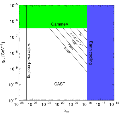
Figure 1: The black lines show the resulting photon fluxes $\phi$ in units of $\mathrm{cm}^{-2}\,\mathrm{s}^{-1}$ for a geoscope with $L=1\,\mathrm{m}$ and $B=10\,\mathrm{T}$ as a function of $\alpha_{ae}$ and $g_{a\gamma}$. The gray lines show the current astro-physical bounds on $\alpha_{ae}$ from the cooling of white dwarfs Amsler:2008zzb and on $g_{a\gamma}$ from the non-observation of solar axions by CAST Andriamonje:2004hi . The colored/shaded regions indicate the parameter space excluded by photon regeneration Chou:2007zzc and the cooling of the Earth (this work).

Before closing, we would like to point out a few directions for improving our estimates. First of all, our picture of the iron core is quite simplified. A more detailed treatment of electron-ion interactions in the molten core, as well as the inner core contribution, which was ignored here, could reveal extra enhancements or suppressions that were left out in our analysis. This could, in principle, require a numerical simulation of the strongly coupled plasma (molten Fe) and the crystalline solid core. Another issue is the possible role that the Fe $3d$-orbital electrons play, given that they are delocalized over a few nuclei and may contribute to pseudo-scattering processes inside the hot Fe medium. Also, there could be important bound-bound and free-bound processes that result in the emission of axions from Fe atoms at high temperatures. These processes have been ignored here, but could provide contributions comparable to those we have estimated. In principle, more detailed geodynamical analyzes may yield stronger bounds on non-convective energy transfer out of the Earth’s core. This can result in tighter bounds on axion-electron coupling $\alpha_{ae}$, in the regime we considered here. Finally, our estimate of a geoscope signal assumed an axion flux transverse to the magnetic field. Given the angular size of the core, as viewed through the geoscope, we expect that effective transverse field is, on average, suppressed by roughly $\cos^{2}30^{\circ}$, which does not affect our conclusions, given the approximate nature of our estimates.

In summary, we have derived estimates on possible emission of axions from the hot core of the Earth. Our analysis allows for possible dependence of axion properties on non-vacuum production media, such as astrophysical environments. We approximated the molten core as a strongly coupled plasma of free degenerate electrons in the background of Fe nuclei. We adapted the existing axion emission estimate from a White Dwarf interior, which is a strongly coupled plasma supported by a degenerate electron gas. We obtained the bound $\alpha_{ae}^{\oplus}\lesssim 10^{-18}$ on the axion-electron coupling, by considering geodynamical constraints on core-cooling rates. Given that geo-axions would originate from a far less extreme environment than stellar cores, our bound is nearly a vacuum bound. Hence, our result improves existing accelerator constraints on $\alpha_{ae}$, in vacuo, by 4 orders of magnitude. We also estimated the signal strength to be expected in a dedicated search for geo-axions using a geoscope, based on magnetic axion-photon conversion.

- (1) R. D. Peccei and H. R. Quinn, Phys. Rev. Lett. 38, 1440 (1977); Phys. Rev. D 16, 1791 (1977).
- (2) J. Preskill, M. B. Wise and F. Wilczek, Phys. Lett. B 120, 127 (1983); L. F. Abbott and P. Sikivie, Phys. Lett. B 120, 133 (1983); M. Dine and W. Fischler, Phys. Lett. B 120, 137 (1983); M. S. Turner, Phys. Rev. D 33, 889 (1986).
- (3) C. Amsler et al. [Particle Data Group], Phys. Lett. B 667, 1 (2008).
- (4) P. Gondolo and G. Raffelt, arXiv:0807.2926 [astro-ph].
- (5) Emission of axions from the core of Jupiter has been considered in: C. Sivaram, Earth, Moon, and Planets 37, 155 (1987).
- (6) A. Liolios, Phys. Lett. B 645, 113 (2007).
- (7) E. Masso and J. Redondo, Phys. Rev. Lett. 97, 151802 (2006) [arXiv:hep-ph/0606163].
- (8) E. Zavattini et al. [PVLAS Collaboration], Phys. Rev. Lett. 96, 110406 (2006) [Erratum-ibid. 99, 129901 (2007)] [arXiv:hep-ex/0507107].
- (9) See, J. Redondo, arXiv:0807.4329 [hep-ph], and references therein.
- (10) G. Cantatore [PVLAS Collaboration], Lect. Notes Phys. 741, 157 (2008).
- (11) P. Sikivie, Phys. Rev. Lett. 51, 1415 (1983) [Erratum-ibid. 52, 695 (1984)].
- (12) K. van Bibber, P. M. McIntyre, D. E. Morris and G. G. Raffelt, Phys. Rev. D 39, 2089 (1989).
- (13) R. D. van der Hilst, et al., Science 315, 1813 (2007).
- (14) E. Clementi and D. L. Raimondi, J. Chem. Phys. 1963, 38, 2686.
- (15) T. Nautiyal and S. Auluck, Phys. Rev. B 32, 6424 (1985).
- (16) G. G. Raffelt, Stars as Laboratories for Fundamental Physics (The University of Chicago Press, 1996).
- (17) G. G. Raffelt, Phys. Lett. B 166, 402 (1986).
- (18) H. Primakoff, Phys. Rev. 81, 899 (1951).
- (19) S. O. Costin and S. L. Butler, Phys. Earth Plan. Int. 157, 55 (2006).
- (20) F. T. . Avignone, arXiv:0810.4917 [nucl-ex].
- (21) K. Zioutas et al. [CAST Collaboration], Phys. Rev. Lett. 94, 121301 (2005) [arXiv:hep-ex/0411033]. S. Andriamonje et al. [CAST Collaboration], JCAP 0704, 010 (2007) [arXiv:hep-ex/0702006].
- (22) See, for example: I. C. Atkinson et al., J. Magn. Reson. Imaging 26: 1222 (2007).
- (23) A. S. Chou et al. [GammeV (T-969) Collaboration], Phys. Rev. Lett. 100, 080402 (2008) [arXiv:0710.3783 [hep-ex]].
- (24) A. J. Miller, et al., Appl. Phys. Lett. 83, 791 (2003).
- (25) A. E. Lita, A. J. Miller, and S. W. Nam, Optics Express 16 3032-3040, (2008).