BPS and non-BPS kinks in a massive non-linear ${\mathbb{S}}^{2}$-sigma model

Abstract

The stability of the topological kinks of the non-linear ${\mathbb{S}}^{2}$-sigma model discovered in AMAJ is discussed by means of a direct estimation of the spectra of the second-order fluctuation operators around topological kinks. The one-loop mass shifts caused by quantum fluctuations around the these kinks are computed using the Cahill-Comtet-Glauber formula CCG . The (lack of) stability of the non-topological kinks is unveiled by application of the Morse index theorem. These kinks are identified as non-BPS states. There are two types of topological kinks coming from the twofold embedding of the sine-Gordon model in the massive non-linear sigma model. It is shown that sine-Gordon kinks of only one type satisfy first-order equations and are accordingly BPS classical solutions. Finally, the interplay between instability and supersymmetry is explored.

I Introduction

The main theme in this paper is the analysis of the structure of the manifold of kink solitary waves discovered in AMAJ . In particular, we shall offer a full description of the stability of the different type of kinks. As a bonus, we shall gain information about the semi-classical behavior of such kinks from the stability analysis, providing us with enough data to compute the one-loop mass shifts for the topological kinks.

Prior to our work AMAJ , kinks in massive non-linear sigma models have been known for some time and profusely studied in different supersymmetric models under the circumstance that all the masses of the pseudo Nambu-Goldstone particles are equal. The study started with two papers by Abraham and Townsend AT , AT1 in which the authors discovered a family of Q-kinks in a (1+1)-dimensional ${\cal N}=(4,4)$ supersymmetric non-linear sigma model with a hyper-Kahler Gibbons-Hawking instanton as the target space and mass terms obtained from dimensional reduction. In Nit , however, these kinks were re-considered by constructing the dimensionally reduced supersymmetric model by means of the mathematically elegant technique of hyper-Kahler quotients. By doing this, the authors deal with massive ${\mathbb{C}P}^{N}$ or ${\mathbb{H}P}^{N}$ models, a playground closer to our simpler massive ${\mathbb{S}}^{2}$-sigma model. Similar ${\cal N}=2$ BPS walls in the ${\mathbb{C}P}^{1}$-model with twisted mass were described in Dor . In a parallel development in the (2+1)-dimensional version of these models, two-dimensional Q-lumps were discovered in Lee and Abr . Throughout this field, the most interesting result is the demonstration in GPTT and INOS that composite solitons in ${\it d}=3+1$ of Q-strings and domain walls are exact BPS solutions that preserve $\frac{1}{4}$ of the supersymmetries: ( See also the review EINOS , where a summary of these supersymmetric topological solitons is offered.)

Our investigation differs from previous work in the area of topological defects in non-linear sigma models in two important aspects: 1) We remain in a purely bosonic framework; in fact, we consider the simplest massive non-linear sigma model. 2) We study the case when the masses of the pseudo Nambu-Goldstone bosons are different. The search for kinks in the (1+1)-dimensional model (domain walls in ${\it d}=3+1$) is tantamount to the search for finite action trajectories in the repulsive Neumann system, a particle moving in an ${\mathbb{S}}^{2}$-sphere under the action of non-isotropic repulsive elastic forces. It is well known that this dynamical system is completely integrable Dub , Per . We show, however, that the problem is Hamilton-Jacobi separable by using elliptic coordinates in the sphere. Use of this allows us to find four families of homoclinic trajectories starting and ending at one of the poles which are unstable points of the mechanical system. In the field-theoretical model the poles become ground states, whereas the homoclinic trajectories correspond to four families of non-topological kinks. Each member in a family is formed by a non-linear combination of two basic topological kinks (of different type) with their centers located at any relative distance with respect each other.

It is remarkable that the static field equations of this massive non-linear sigma model are (almost) the static Landau-Lifshitz equations governing the high spin and long wavelength limit of $1D$ ferromagnetic materials. From this perspective, topological kinks can be interpreted respectively as Bloch and Ising walls that form interfaces between ferromagnetic domains, similar to those discovered in the XY model dealt with in BW . The variety of our non-topological kinks, understood as solitary spin waves, is thus formed by non-linear superpositions of one basic Bloch wall and one basic Ising wall at different distances. Far from this non-relativistic context, degenerate Bloch/Ising branes have been studied in two-scalar field theories coupled to gravity in ES ; BG ; SAH .

II The (1+1)-dimensional massive non-linear ${\mathbb{S}}^{2}$-sigma model

We shall focus on the non-linear ${\mathbb{S}}^{2}$-sigma model studied in Reference AMAJ . The action governing the dynamics is:

$$S[\phi_{1},\phi_{2},\phi_{3}]=\int\,dtdx\,\left\{{1\over 2}g^{\mu\nu}\sum_{a=1}^{3}\frac{\partial\phi_{a}}{\partial x^{\mu}}\frac{\partial\phi_{a}}{\partial x^{\nu}}-V\right\},$$ (1)

with $V=V(\phi_{1}(t,x),\phi_{2}(t,x),\phi_{3}(t,x))$. The scalar fields are constrained to satisfy: $\phi_{1}^{2}+\phi_{2}^{2}+\phi_{3}^{2}=R^{2}$, and thus $\phi_{a}(t,x)\in{\rm Maps}({\mathbb{R}}^{1,1},{\mathbb{S}}^{2})$ are maps from the $(1+1)$-dimensional Minkowski space-time to a ${\mathbb{S}}^{2}$-sphere of radius $R$, which is the target manifold of the model.

Our conventions for ${\mathbb{R}}^{1,1}$ are as follows: $x^{\mu}\in{\mathbb{R}}^{1,1}$, $\mu=0,1$, $x^{\mu}\cdot x_{\mu}=g^{\mu\nu}x_{\mu}x_{\nu}$, $g^{\mu\nu}={\rm diag}(1,-1)$. $x^{0}=t$, $x^{1}=x$, $x^{\mu}\cdot x_{\mu}=t^{2}-x^{2}$; $\partial_{\mu}\partial^{\mu}=g^{\mu\nu}\partial_{\mu\nu}^{2}=\Box=\partial_{t}^{2}-\partial_{x}^{2}$.

The infrared asymptotics of $(1+1)$-dimensional scalar field theories forbids massless particles, see Col . We thus choose the simplest potential energy density that would be generated by quantum fluctuations giving mass to the fundamental quanta:

$$V(\phi_{1},\phi_{2},\phi_{3})=\frac{1}{2}\left(\alpha_{1}^{2}\,\phi_{1}^{2}+\alpha_{2}^{2}\,\phi_{2}^{2}+\alpha_{3}^{2}\,\phi_{3}^{2}\right),$$ (2)

which we set with no loss of generality such that: $\alpha_{1}^{2}\geq\alpha_{2}^{2}>\alpha_{3}^{2}\geq 0$.

1. Solving $\phi_{3}$ in favor of $\phi_{1}$ and $\phi_{2}$, $\phi_{3}={\rm sg}(\phi_{3})\sqrt{R^{2}-\phi_{1}^{2}-\phi_{2}^{2}}$, we find:

$$S={1\over 2}\int\,dtdx\,\left\{\partial_{\mu}\phi_{1}\partial^{\mu}\phi_{1}+\partial_{\mu}\phi_{2}\partial^{\mu}\phi_{2}+\right.$$

$$\left.\frac{(\phi_{1}\partial_{\mu}\phi_{1}+\phi_{2}\partial_{\mu}\phi_{2})(\phi_{1}\partial^{\mu}\phi_{1}+\phi_{2}\partial^{\mu}\phi_{2})}{R^{2}-\phi_{1}^{2}-\phi_{2}^{2}}-2V_{{\mathbb{S}}^{2}}(\phi_{1},\phi_{2})\right\}$$

$$V_{{\mathbb{S}}^{2}}(\phi_{1},\phi_{2})=\frac{1}{2}\left((\alpha_{1}^{2}-\alpha_{3}^{2})\,\phi_{1}^{2}+(\alpha_{2}^{2}-\alpha_{3}^{2})\,\phi_{2}^{2}+{\rm const.}\right)$$

$$\hskip 28.45274pt\simeq\frac{\lambda^{2}}{2}\phi_{1}^{2}(t,x)+\frac{\gamma^{2}}{2}\phi_{2}^{2}(t,x)$$ (3)

with $\lambda^{2}=(\alpha_{1}^{2}-\alpha_{3}^{2})$, $\gamma^{2}=(\alpha_{2}^{2}-\alpha_{3}^{2})$, $\lambda^{2}\geq\gamma^{2}$.

2. Thus, the interactions come from the geometry:

$$\frac{(\phi_{1}\partial_{\mu}\phi_{1}+\phi_{2}\partial_{\mu}\phi_{2})(\phi_{1}\partial^{\mu}\phi_{1}+\phi_{2}\partial^{\mu}\phi_{2})}{R^{2}-\phi_{1}^{2}-\phi_{2}^{2}}\simeq$$

$$\simeq {1\over R^{2}}\left(1+{1\over R^{2}}(\phi_{1}^{2}+\phi_{2}^{2})+{1\over R^{4}}(\phi_{1}^{2}+\phi_{2})^{2}+\cdots\right)\cdot$$

$$\cdot\left(\phi_{1}\partial_{\mu}\phi_{1}+\phi_{2}\partial_{\mu}\phi_{2}\right)\left(\phi_{1}\partial^{\mu}\phi_{1}+\phi_{2}\partial^{\mu}\phi_{2}\right)\quad,$$

and ${1\over R^{2}}$ is a non-dimensional coupling constant, whereas the masses of the pseudo-Nambu-Goldstone bosons are respectively $\lambda$ and $\gamma$.

Taking into account that in the natural system of units $\hbar=c=1$ the dimensions of fields, masses and coupling constants are $[\phi_{a}]=1=[R]$, $[\gamma]=M=[\lambda]$, we define the non-dimensional space-time coordinates and masses

$$x^{\mu}\,\rightarrow\,\frac{x^{\mu}}{\lambda},\,\sigma^{2}=\frac{\alpha_{2}^{2}-\alpha_{3}^{2}}{\alpha_{1}^{2}-\alpha_{3}^{2}}=\frac{\gamma^{2}}{\lambda^{2}},\quad 0<\sigma^{2}\leq 1,$$

to write the energy in terms of them:

$$E= {\lambda\over 2}\int\,dx\,\left\{\left(\partial_{t}\phi_{1}\right)^{2}+\left(\partial_{t}\phi_{2}\right)^{2}+\left(\partial_{x}\phi_{1}\right)^{2}+\left(\partial_{x}\phi_{2}\right)^{2}\right.$$ (4)

$$+\frac{(\phi_{1}\partial_{t}\phi_{1}+\phi_{2}\partial_{t}\phi_{2})^{2}+(\phi_{1}\partial_{x}\phi_{1}+\phi_{2}\partial_{x}\phi_{2})^{2}}{R^{2}-\phi_{1}^{2}-\phi_{2}^{2}}$$

$$+\left.\phi_{1}^{2}(t,x)+\sigma^{2}\cdot\phi_{2}^{2}(t,x)\right\}\ \ \,.$$

In the time-independent homogeneous minima of the action or vacua of our model, $\phi_{1}^{V^{\pm}}=\phi_{2}^{V^{\pm}}=0$, $\phi_{3}^{V^{\pm}}=\pm R$ (North and South Poles), the ${\mathbb{Z}}_{2}\times{\mathbb{Z}}_{2}\times{\mathbb{Z}}_{2}$, $\phi_{a}\rightarrow(-1)^{\delta_{ab}}\phi_{b}$, $b=1,2,3$ symmetry of the action (1) is spontaneously broken to: ${\mathbb{Z}}_{2}\times{\mathbb{Z}}_{2}$, $\phi_{\alpha}\rightarrow(-1)^{\delta_{\alpha\beta}}\phi_{\beta}$, $\alpha,\,\beta=1,2$. Finite energy configurations require:

$$\lim_{x\to\pm\infty}\frac{d\phi_{\alpha}}{dx}=0\qquad,\qquad\lim_{x\to\pm\infty}\phi_{\alpha}=0\qquad.$$ (5)

Therefore, the configuration space ${\cal C}=\left\{{\rm Maps}({\mathbb{R}},{\mathbb{S}}^{2})/\right.$ $\left.E<+\infty\right\}$ is the union of four disconnected sectors ${\cal C}={\cal C}_{\rm NN}\bigcup{\cal C}_{\rm SS}\bigcup{\cal C}_{\rm NS}\bigcup{\cal C}_{\rm SN}$ labeled by the vacua reached by each configuration at the two disconnected components of the boundary of the real line.

We now solve the constraint by using spherical coordinates: $\theta\in[0,\pi]$, $\varphi\in[0,2\pi)$

$$\phi_{1}(t,x) = R\sin\theta(t,x)\cos\varphi(t,x)$$

$$\phi_{2}(t,x) = R\sin\theta(t,x)\sin\varphi(t,x)$$

$$\phi_{3}(t,x) = R\cos\theta(t,x)\,\,\,.$$

In spherical coordinates the mass terms (we shall denote in the sequel: $\bar{\sigma}=\sqrt{1-\sigma^{2}}$) are

$$V(\theta,\varphi)=\frac{R^{2}}{2}\sin^{2}\theta(\sigma^{2}+\bar{\sigma}^{2}\cos^{2}\varphi)\qquad,$$ (6)

the action becomes

$$S=\int dtdx \left\{\frac{R^{2}}{2}\left[\partial_{\mu}\theta\partial^{\mu}\theta+\sin^{2}\theta\partial_{\mu}\varphi\partial^{\mu}\varphi\right]\right.$$

$$\left.-\frac{R^{2}}{2}\sin^{2}\theta(\sigma^{2}+\bar{\sigma}^{2}\cos^{2}\varphi)\right\}\qquad,$$

and the field equations read:

$$\Box\theta-{1\over 2}{\rm sin}2\theta\left(\partial^{\mu}\varphi\partial_{\mu}\varphi-\cos^{2}\varphi-\sigma^{2}\sin^{2}\varphi\right) = 0$$ (7)

$$\partial^{\mu}(\sin^{2}\theta\partial_{\mu}\varphi)-{1\over 2}\bar{\sigma}^{2}\sin^{2}\theta\sin 2\varphi = 0\,.$$ (8)

Finite energy solutions for which the space-time dependence is of the form:

$$\theta(t,x)=\theta\left(\frac{x-vt}{\sqrt{1-v^{2}}}\right),\quad\varphi(t,x)=\varphi\left(\frac{x-vt}{\sqrt{1-v^{2}}}\right),$$

for some velocity $v$, are called solitary waves. Lorentz invariance allows us to obtain all the solitary waves in our model from solutions of the static field equations

$$\theta^{\prime\prime}-{1\over 2}\sin 2\theta\,(\varphi^{\prime})^{2} = {1\over 2}\left(\cos^{2}\varphi+\sigma^{2}\sin^{2}\varphi\right)\sin 2\theta$$ (9)

$$\frac{d}{dx}(\sin^{2}\theta\,\varphi^{\prime}) = {1\over 2}\bar{\sigma}^{2}\sin^{2}\theta\sin 2\varphi\qquad,$$ (10)

where the notation is: $\theta^{\prime}=\frac{d\theta}{dx}$, $\varphi^{\prime}=\frac{d\varphi}{dx}$. The energy of the static configurations is:

$$E[\theta,\phi]=\lambda\int\,dx\ {\cal E}(\theta^{\prime}(x),\varphi^{\prime}(x),\theta(x),\varphi(x))\ ,$$

$${\cal E}=\frac{\lambda R^{2}}{2}\left((\theta^{\prime})^{2}+\sin^{2}\theta(\varphi^{\prime})^{2}+\sin^{2}\theta(\sigma^{2}+\bar{\sigma}^{2}\cos^{2}\varphi)\right)\,\,.$$

III Topological kinks

Equation (8) is satisfied for constant values of $\varphi$ if and only if: $\varphi=0,\frac{\pi}{2},\pi,\frac{3\pi}{2}$. Depending on which pair of $\varphi$-constant solution we choose, (7) becomes one or another sine-Gordon equation:

$$\Box\theta+{\sigma^{2}\over 2}\sin 2\theta=0\ ;\quad\Box\theta+{1\over 2}\sin 2\theta=0\qquad.$$

Thus, sine-Gordon models are embedded in our system on these two orthogonal meridians.

 

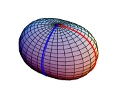
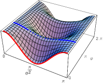
Figure 1: a) $V(\theta,\varphi)$ deformation of ${\mathbb{S}}^{2}$, b) Embedding of the sine-Gordon model at $\varphi=0$, $\varphi=\frac{\pi}{2}$ as seen in $-V(\theta,\varphi)$.

1. $K_{1}/K_{1}^{*}$ kinks. We denote $K_{1}/K_{1}^{*}$ the kink/antikink solutions of the sG model embedded inside the ${\mathbb{S}}^{2}$ model in the $\varphi_{K_{1}}(x)={\pi\over 2}$ or $\varphi_{K_{1}^{*}}(x)={3\pi\over 2}$ two halves of the single meridian intersecting the $\phi_{2}:\phi_{3}$ plane,

$$\theta_{K_{1}}(x)=\theta_{K_{1}^{*}}(x)=2\arctan\,e^{\pm\sigma(x-x_{0})}\qquad,$$ (11)

see Figure 1. The energy of these kinks, which belong to ${\cal C}_{\rm NS}$ (kinks) or ${\cal C}_{\rm SN}$ (antikinks), is: $E^{C}_{K_{1}}=E^{C}_{K_{1}^{*}}=2\lambda R^{2}\sigma$.

2. $K_{2}/K_{2}^{*}$ kinks. Taking $\varphi_{K_{2}}(x)=0$ or $\varphi_{K_{2}^{*}}(x)=\pi$, we find the sG kinks:

$$\theta_{K_{2}}(x)=\theta_{K_{2}^{*}}(x)=2\arctan e^{\pm(x-x_{0})}\,\,.$$ (12)

The energy of the $K_{2}/K_{2}^{*}$ kinks, which also belong to the ${\cal C}_{\rm NS}$, ${\cal C}_{\rm SN}$ sectors, is greater than the energy of the $K_{1}/K_{1}^{*}$ kinks: $E^{C}_{K_{2}}=E^{C}_{K_{2}^{*}}=2\lambda R^{2}$.

3. Degenerate families of $Q_{\alpha}$-kinks. When $\sigma^{2}=1$, the system enjoys $SO(2)$ internal symmetry and the masses of the two pseudo-Nambu-Goldstone bosons are equal, there are degenerate families of time-dependent $Q$-kinks of finite energy. If $\sigma=1$: $\varphi^{Q_{\alpha}}(t)=\omega t+\alpha$, where $\omega$ and $\alpha$ are real constants, solves (8) for any time-independent $\theta(x)$. Moreover, by plugging $\varphi^{Q_{\alpha}}(t)$ into (7) one obtains:

$$\theta^{Q_{\alpha}}(x)=2\arctan e^{\pm\sqrt{1-\omega^{2}}(x-x_{0})},\ \forall\alpha.$$ (13)

Therefore, if $0<\omega^{2}<1$, the $(\theta^{Q_{\alpha}}(x),\varphi^{Q_{\alpha}}(t))$ configurations form a degenerate circle of periodic in time Q-kink solutions of energy:

$$E^{C}_{Q_{\alpha}}=\frac{2\lambda R^{2}}{\sqrt{1-\omega^{2}}}=\frac{2\lambda R^{2}}{\bar{\omega}}\,\,\,\,,\,\,\,\,\forall\alpha\ .$$

In fact, these $Q$-kinks can be viewed as the sG kinks rotating around the main axis of ${\mathbb{S}}^{2}$ with constant angular velocity $\omega$. In another reference frame moving with respect to the $Q_{\alpha}$-kink CM with velocity $v$, the interplay between $x$ and $t$ dependence is more complicated:

$$\varphi^{Q_{\alpha}}(x,t)=\omega\left(\frac{t-vx}{\sqrt{1-v^{2}}}\right)+\alpha$$

$$\theta^{Q_{\alpha}}(x,t)=2\arctan e^{\pm\bar{\omega}\left(\frac{x-vt}{\sqrt{1-v^{2}}}-x_{0}\right)}.$$

At the $\omega=0$ limit we find a circle of static topological kinks that form a degenerate family of solitary waves of the system.

Of course, all the multi-soliton, soliton-antisoliton and breather solutions of the sG model are also solitons of our system in the meridians intersecting either the $\phi_{2}:\phi_{3}$ or the $\phi_{1}:\phi_{3}$ planes. We shall not discuss these solutions in this work and postpone their study to a future research.

IV Topological kink stability

IV.1 Small fluctuations on topological kinks

The analysis of small fluctuations around topological kinks requires us to consider both the geodesic deviation operator and the Hessian of the potential energy density. We will denote $\theta=\theta^{1}\in[0,\pi]$, $\varphi=\theta^{2}\in[0,2\pi)$, and thus the arc-length reads: $ds^{2}=R^{2}d\theta^{1}d\theta^{1}+R^{2}\sin^{2}\theta^{1}d\theta^{2}d\theta^{2}$. We also denote the Kink trajectories and small deformations around them as: $\theta_{K}(x)=(\theta^{1}_{K}(x)=\bar{\theta},\theta^{2}_{K}(x)=\bar{\varphi})$, $\theta(x)=\theta_{K}(x)+\eta(x)$, $\eta(x)=(\eta^{1}(x),\eta^{2}(x))$.

Let us consider the following contra-variant vector fields along the kink trajectory, $\eta,\theta^{\prime}_{K}\in\Gamma(T{\mathbb{S}}^{2}\left|{}_{K}\right.)$: $\eta(x)=\eta^{1}(x)\frac{\partial}{\partial\theta^{1}}+\eta^{2}(x)\frac{\partial}{\partial\theta^{2}}$ and $\theta^{\prime}_{K}(x)=\bar{\theta}^{\prime}\frac{\partial}{\partial\theta^{1}}+\bar{\varphi}^{\prime}\frac{\partial}{\partial\theta^{2}}$.

The covariant derivative of $\eta(x)$ and the action of the curvature tensor on $\eta(x)$ are:

$$\nabla_{\theta_{K}^{\prime}}\eta=\left(\eta^{\prime i}(x)+\Gamma^{i}_{jk}\eta^{j}\bar{\theta}^{\prime k}\right)\frac{\partial}{\partial\theta^{i}}$$

$$R(\theta^{\prime}_{K},\eta)\theta^{\prime}_{K}=\bar{\theta}^{\prime i}\eta^{j}(x)\bar{\theta}^{\prime k}R^{l}_{ijk}\frac{\partial}{\partial\theta^{l}}.$$

The geodesic deviation operator is:

$$\frac{D^{2}\eta}{dx^{2}}+R(\theta^{\prime}_{K},\eta)\theta^{\prime}_{K}=\nabla_{\theta_{K}^{\prime}}\nabla_{\theta_{K}^{\prime}}\eta+R(\theta^{\prime}_{K},\eta)\theta^{\prime}_{K}\ .$$

To obtain the differential operator that governs the second-order fluctuations around the kink $\theta_{K}$, the remaining ingredient is the Hessian of the potential:

$$\nabla_{\eta}{\rm grad}V=\eta^{i}\left(\frac{\partial^{2}V}{\partial\theta^{i}\partial\theta^{j}}-\Gamma^{k}_{ij}\frac{\partial V}{\partial\theta^{k}}\right)g^{jl}\frac{\partial}{\partial\theta^{l}}$$

evaluated at $\theta_{K}(x)$. In sum, second-order kink fluctuations are determined by the operator:

$$\Delta_{K}\eta=-\left(\nabla_{\theta_{K}^{\prime}}\nabla_{\theta_{K}^{\prime}}\eta+R(\theta^{\prime}_{K},\eta)\theta^{\prime}_{K}+\nabla_{\eta}{\rm grad}V\right)$$ (14)

IV.2 The spectrum of small fluctuations around $K_{1}/K_{1}^{*}$ kinks

Plugging the $K_{1}$ solutions into (14), we obtain the differential operator acting on the second-order fluctuation operator around the $K_{1}/K_{1}^{*}$ kinks:

$$\Delta_{K_{1}}\eta = \Delta_{K_{1}^{*}}\eta=\left[-\frac{d^{2}\eta^{1}}{dx^{2}}+\left(\sigma^{2}-\frac{2\sigma^{2}}{{\rm cosh}^{2}\sigma x}\right)\eta^{1}\right]\frac{\partial}{\partial\theta^{1}}$$ (15)

$$+\left[-\frac{d^{2}\eta^{2}}{dx^{2}}+2\sigma{\rm tanh}\sigma x\frac{d\eta^{2}}{dx}+\bar{\sigma}^{2}\eta^{2}\right]\frac{\partial}{\partial\theta^{2}}\ .$$

The vector fields $v(x)=v^{1}(x)\frac{\partial}{\partial\theta^{1}}+v^{2}(x)\frac{\partial}{\partial\theta^{2}}$ parallel along the $K_{1}$ kink orbits satisfy: $\frac{dv^{i}}{dx}+\Gamma^{i}_{jk}\bar{\theta}^{\prime j}v^{k}=0$, or,

$$\left\{\begin{array}[]{cc}\frac{dv^{1}}{dx}=0&,\,\,\,v^{1}(x)=1\\[5.69046pt] \frac{dv^{2}}{dx}+\sigma\frac{{\rm cotan}(2{\rm arctan}e^{\sigma x})}{{\rm cosh}\sigma x}v^{2}=0&\,\,,\,\,\,v^{2}(x)={\rm cosh}\sigma x\end{array}\right.\quad.$$

Therefore, $v_{1}=\frac{\partial}{\partial\theta^{1}}\,\,\,,\,\,\,v_{2}(x)=\cosh\sigma x\,\frac{\partial}{\partial\theta^{2}}$ is a frame $\left\{v_{1},v_{2}\right\}$ in $\Gamma(T{\mathbb{S}}^{2}|_{K_{1}})$ parallel to the $K_{1}$ kink orbit in which (15) reads:

$$\Delta_{K_{1}}\eta = \Delta_{K_{1}^{*}}\eta=\left[-\frac{d^{2}\bar{\eta}^{1}}{dx^{2}}+(\sigma^{2}-\frac{2\sigma^{2}}{\cosh^{2}\sigma x})\bar{\eta}^{1}\right]\,v_{1}$$ (16)

$$+ \left[-\frac{d^{2}\bar{\eta}^{2}}{dx^{2}}+(1-\frac{2\sigma^{2}}{\cosh^{2}\sigma x})\bar{\eta}^{2}\right]\,v_{2}\quad,$$

where $\eta=\bar{\eta}^{1}\,v_{1}+\bar{\eta}^{2}\,v_{2}$, $\eta^{1}=\bar{\eta}^{1}$, and $\eta^{2}=\cosh\sigma x\,\bar{\eta}^{2}$.

The second-order fluctuation operator (16) is a diagonal matrix of transparent Pösch-Teller Schrödinger operators with very well known spectra. As expected, despite the geometric nature of $\bigtriangleup_{K_{1}}$, we find in the $v_{1}=\frac{\partial}{\partial\theta^{1}}$ direction the Schrödinger operator governing sG kink fluctuations. Finding another Pösch-Teller potential of the same type in the $v_{2}=\frac{\partial}{\partial\theta^{2}}$ direction comes out as a surprise because there is no a priori reason for such a behavior in the orthogonal direction.

In the $v_{1}$ direction there is a bound state of zero eigenvalue and a continuous family of positive eigenfunctions:

$$\bar{\eta}^{1}_{0}(x)=\mathop{\rm sech}\nolimits\sigma x \varepsilon^{(1)}_{0}=0$$ ,

$$\bar{\eta}^{1}_{k}(x)=e^{ik\sigma x}({\rm tanh}\sigma x-ik) \varepsilon^{(1)}(k)=\sigma^{2}(k^{2}+1)\ .$$ ,

In the $v_{2}=\cosh\sigma x\frac{\partial}{\partial\theta^{2}}$ direction the spectrum is similar but the bound state corresponds to a positive eigenvalue:

$$\bar{\eta}^{2}_{1-\sigma^{2}}(x)=\mathop{\rm sech}\nolimits\sigma x \varepsilon^{(2)}_{1-\sigma^{2}}=1-\sigma^{2}>0$$ ,

$$\bar{\eta}^{2}_{k}(x)=e^{ik\sigma x}({\rm tanh}\sigma x-ik) \varepsilon^{(2)}(k)=\sigma^{2}k^{2}+1\ .$$ ,

Because there are no fluctuations of negative eigenvalue, the $K_{1}/K_{1}^{*}$ kinks are stable.

IV.3 One-loop shift to classical $K_{1}/K_{1}^{*}$ kink masses

The reflection coefficient of the scattering waves in the potential wells of the Schrödinger operators in (16) being zero, it is possible to use the Cahill-Comtet-Glauber formula CCG (see also BC for a more detailed derivation) to compute the quantum correction to the $K_{1}$ classical kink mass up to one-loop order:

$$E_{K_{1}}(\sigma) = E^{C}_{K_{1}}(\sigma)+\Delta E_{K_{1}}(\sigma)+{\cal O}(\frac{1}{R^{2}})=$$ (17)

$$= 2\lambda R^{2}\sigma-\frac{\lambda\sigma}{\pi}[\sin\nu_{1}+{1\over\sigma}\sin\nu_{2}-\nu_{1}\cos\nu_{1}$$

$$-{1\over\sigma}\nu_{2}\cos\nu_{2}]+{\cal O}(\frac{1}{R^{2}})$$

In (17) $\nu_{1}=\arccos 0={\pi\over 2}$, $\nu_{2}=\arccos\bar{\sigma}$, are determined from the eigenvalues of the bound states and the thresholds of the continuous spectra. This simple structure of the one-loop kink mass shift occurs only for transparent potentials. In our model, we find the formula:

$$E_{K_{1}}(\sigma)=2\lambda R^{2}\sigma-\frac{\lambda\sigma}{\pi}\left[2-\frac{\bar{\sigma}}{\sigma}\arccos(\bar{\sigma})\right]+{\cal O}(\frac{1}{R^{2}})$$ (18)

For instance, for $\sigma={1\over 2}$ we obtain a result similar to the mass shift of the $\lambda\phi^{4}_{2}$-kink:

$$E_{K_{1}}(\frac{1}{2})=\lambda R^{2}-\frac{3\lambda}{2\pi}\left(\frac{2}{3}-\frac{\pi}{6\sqrt{3}}\right)+{\cal O}(\frac{1}{R^{2}})$$

As in the $\lambda\phi^{4}_{2}$-kink case, a zero mode and a bound eigenstate of eigenvalue $\varepsilon_{3\over 4}^{(2)}={3\over 4}$ contribute. The gaps between the bound state eigenvalues and the thresholds $\varepsilon^{(1)}(0)=\sigma^{2}$, $\varepsilon^{(2)}(0)=1$ of the two branches of the continuous spectrum are the same in our model. The gaps, however, are different from the gaps in the $\lambda\phi^{4}_{2}$ model between the eigenvalues of the two bound states and the threshold of the only branch of the continuous spectrum. Both features contribute to the slightly different result. The $\sigma=1$ symmetric case is more interesting. We find exactly twice the spectrum of the sG kink: two zero modes and two gaps with respect to the thresholds of the continuous spectrum equal to one. No wonder that the one-loop mass shifts of the degenerate kinks is twice the one-loop correction of the sG kink:

$$E_{K_{\alpha}}(1)=2\lambda\left(R^{2}-{1\over\pi}\right)+{\cal O}(\frac{1}{R^{2}}),\ \forall\alpha\,\,!\,\,.$$

Moreover, the quantum fluctuations do not break the $SO(2)$-symmetry and our result fits in perfectly well with the one-loop shift to the mass of the ${\cal N}=(2,2)$ SUSY ${\mathbb{C}P}^{1}$ kink computed in MRNW where the authors find twice the mass of the ${\cal N}=1$ SUSY sine-Gordon kink. A different derivation of formula (18) following the procedure of AMAWJ1 , see also AMAWJ2 ; AMAWJ3 , will be published elsewhere.

IV.4 The spectrum of small fluctuations around $K_{2}/K_{2}^{*}$ kinks

By inserting the $K_{2}$ solutions in (14) the second-order fluctuation operator around the $K_{2}/K_{2}^{*}$ kinks is found:

$$\Delta_{K_{2}}\eta=\Delta_{K_{2}^{*}}\eta=\left[-\frac{d^{2}\eta^{1}}{dx^{2}}+(1-\frac{2}{{\rm cosh}^{2}x})\eta^{1}\right]\frac{\partial}{\partial\theta^{1}}$$

$$+\left[-\frac{d^{2}\eta^{2}}{dx^{2}}+2\tanh x\frac{d\eta^{2}}{dx}-\bar{\sigma}^{2}\eta^{2}\right]\frac{\partial}{\partial\theta^{2}}\ .$$ (19)

Solving again the parallel transport equations, now along the $K_{2}$ solutions, it is obtained the parallel frame: $\{u_{1},u_{2}\}\in\Gamma(T{\mathbb{S}}^{2}\left|{}_{K_{2}})\right.$, $u_{1}=\frac{\partial}{\partial\theta^{1}}$, $u_{2}(x)=\cosh x\,\frac{\partial}{\partial\theta^{2}}$, to the $K_{2}/K_{2}^{*}$ orbits. (19) becomes:

$$\Delta_{K_{2}}\eta = \Delta_{K_{2}^{*}}\eta=\left[-\frac{d^{2}\tilde{\eta}^{1}}{dx^{2}}+(1-\frac{2}{\cosh^{2}x})\tilde{\eta}^{1}\right]u_{1}$$ (20)

$$+ \left[-\frac{d^{2}\tilde{\eta}^{2}}{dx^{2}}+(\sigma^{2}-\frac{2}{\cosh^{2}x})\tilde{\eta}^{2}\right]u_{2}\ .$$

with $\eta=\tilde{\eta}^{1}u_{1}+\tilde{\eta}^{2}u_{2}$, $\eta^{1}=\tilde{\eta}^{1}$, $\eta^{2}=\cosh x\tilde{\eta}^{2}$.

Again, the second-order fluctuation operator (19) is a diagonal matrix of transparent Pösch-Teller operators. In this case, there is a bound state of zero eigenvalue and a continuous family of positive eigenfunctions starting at the threshold $\varepsilon^{(1)}(0)=1$ in the $u_{1}=\frac{\partial}{\partial\theta^{1}}$ direction:

$$\tilde{\eta}^{1}_{0}(x)=\mathop{\rm sech}\nolimits x \varepsilon^{(1)}_{0}=0$$ ,

$$\tilde{\eta}^{1}_{k}(x)=e^{ikx}(\tanh x-ik) \varepsilon^{(1)}(k)=(k^{2}+1)\ ,$$ ,

as corresponds to the sG kink. In the $u_{2}(x)=\cosh x\frac{\partial}{\partial\theta^{2}}$ direction, the spectrum is similar but the eigenvalue of the bound state is negative, whereas the threshold of this branch of the continuous spectrum is $\varepsilon^{(2)}(0)=\sigma^{2}$:

$$\tilde{\eta}^{2}_{\sigma^{2}-1}(x)=\mathop{\rm sech}\nolimits x \varepsilon^{(2)}_{\sigma^{2}-1}=\sigma^{2}-1<0$$ ,

$$\tilde{\eta}^{2}_{k}(x)=e^{ikx}(\tanh x-ik) \varepsilon^{(2)}(k)=k^{2}+\sigma^{2}\ .$$ ,

Therefore, $K_{2}/K_{2}^{*}$ kinks are unstable and a Jacobi field for $k=i\sigma$ arises: $\tilde{\eta}^{2}_{J}(x)=e^{\sigma x}(\tanh x-\sigma)$, $\varepsilon^{(2)}_{J}=0$.

IV.5 One-loop shift to classical $K_{2}/K_{2}^{*}$ kink masses

Once again we use the Cahill-Comtet-Glauber formula to compute the quantum correction to the $K_{2}$ classical kink mass up to one-loop order. As before, the angles $\nu_{1}=\arccos(0)$ $={\pi\over 2}$, $\nu_{2}=$ $\arccos(i\bar{\sigma})$, are determined from the eigenvalues of the bound states and the thresholds of the continuous spectra. The novelty is that since the bound state eigenvalue is negative $\nu_{2}$ is purely imaginary. Therefore, we find:

$$E_{K_{2}}(\sigma)=2\lambda R^{2}-\frac{\lambda\sigma}{\pi}\left[{1\over\sigma}+\sqrt{2-\sigma^{2}}-i{\pi\over 2}\bar{\sigma}\right.$$

$$\left.+\bar{\sigma}\log\left[\sqrt{2-\sigma^{2}}-\bar{\sigma}\right]\right]+{\cal O}(\frac{1}{R^{2}})\ .$$ (21)

The key point is that the one-loop mass shift is a complex quantity, the imaginary part telling us about the life-time of this resonant state. In the $\sigma=1$ symmetric case, however, we find the expected purely real answer: $E_{K_{2}}(1)=2\lambda\left(R^{2}-{1\over\pi}\right)+{\cal O}(\frac{1}{R^{2}})$.

IV.6 BPS $Q_{\alpha}$-kinks as $d=1+1$ dyons

In the $\sigma^{2}=1$ case there is symmetry with respect to the ${\rm exp}[\alpha{\tiny\left(\begin{array}[]{ccc}0&-1&0\\ 1&0&0\\ 0&0&0\end{array}\right)}]\in{\mathbb{S}O}(2)$ subgroup of the ${\mathbb{O}}(3)$ group. The associated Nöether charge distinguishes between different $Q_{\alpha}$-kinks :

$$Q=\frac{1}{2}\int\,dx\,(\phi_{1}\partial_{t}\phi_{2}-\phi_{2}\partial_{t}\phi_{1})=R^{2}\int\,dx\,\sin^{2}\theta\partial_{t}\varphi$$

$$Q[Q_{\alpha}]=R^{2}\omega\int\,dx\,\sin^{2}\theta^{Q_{\alpha}}=2R^{2}\frac{\omega}{\bar{\omega}}\ .$$

For configurations such that $\theta$ is time-independent and $\varphi$ is space-independent, the energy can be written as:

$$E = \frac{\lambda R^{2}}{2}\int\,dx\,\left\{\sin^{2}\theta[\dot{\varphi}-\omega]^{2}+[\theta^{\prime}\pm\bar{\omega}\sin\theta]^{2}\right\}$$ (22)

$$+ \lambda R^{2}\int\,dx\,\left\{\omega\sin^{2}\theta\dot{\varphi}\mp\bar{\omega}\theta^{\prime}\sin\theta\right\}\ ,$$

($\dot{\varphi}=\frac{d\varphi}{dt}(t)$), in such a way that the solutions of the first-order equations:

$$\dot{\varphi}=\omega\,\Rightarrow\,\varphi^{Q_{\alpha}}(t)=\omega t+\alpha$$

$$\theta^{\prime}=\mp\bar{\omega}\sin\theta\,\Rightarrow\,\theta^{Q_{\alpha}}(x)=2\arctan e^{\mp\bar{\omega}(x-x_{0})}\ ,$$

the $Q_{\alpha}$-kinks, saturate the Bogomolny bound and are BPS:

$$E_{\rm BPS}=\frac{2\lambda R^{2}}{\bar{\omega}}=\lambda\left\{\omega Q+\bar{\omega}T\right\}.$$ (23)

Here, the topological charge $T=|W[\theta(+\infty,t)]-W[\theta(-\infty,t)]|$ coming from the superpotential $W=R^{2}(1\mp\cos\theta)$ valued at the $Q_{\alpha}$-kinks gives: $T[Q_{\alpha}]=2R^{2},\forall\alpha$. This explains why “one cannot dent a dyon” (even a one-dimensional cousin), see CPNS . Conservation of the Nöether charge forbids the decay of $Q_{\alpha}$ kinks, all of them living in the same topological sector, to others with less energy.

IV.7 Bohr-Sommerfeld rule: $Q$-kink energy and charge quantization

The Bohr-Sommerfeld quantization rule applied to periodic in time-classical solutions in our model reads:

$$\int_{0}^{T}\,dt\,\int\,dx\,\pi_{\varphi}(t,x)\frac{\partial\varphi}{\partial t}(t,x)$$

$$=R^{2}\int_{0}^{T}\,dt\,\int\,dx\,\sin^{2}\theta(x,t)\frac{\partial\varphi}{\partial t}\frac{\partial\varphi}{\partial t}=2\pi n\,\,.$$

In Col1 it is explained how derivation of this formula with respect to the period $T=\frac{2\pi}{\omega}$ leads to the ODE: $\lambda\frac{dn}{dE}=\omega^{-1}(E)$, or,

$$\lambda\int_{0}^{n}\,dn=\int_{E_{0}}^{E_{n}}\,\frac{EdE}{\sqrt{E^{2}-4\lambda^{2}R^{4}}}\Rightarrow E_{n}=\lambda\sqrt{n^{2}+4R^{4}}$$

starting from $E_{0}=2\lambda R^{2}$ and assuming $n$ to be a positive integer. The $Q$-kink energy is thus quantized and the frequencies and charges allowed by the Bohr-Sommerfeld rule form also a numerable infinite set:

$$\omega_{n}=\sqrt{1-\frac{1}{1+\frac{n^{2}}{4R^{4}}}}\quad,\quad Q_{n}=n\,\,\,\,.$$

V The massive non-linear ${\mathbb{S}}^{2}$-sigma model in spherical elliptic coordinates

The secret of this non-linear (1+1)-dimensional massive ${\mathbb{S}}^{2}$-sigma model is that its analogous mechanical system is Hamilton-Jacobi separable in spherical elliptic coordinates. This fact will allow us to known explicitly not only the kink solutions inherited from the embedded sG models, but the complete set of solitary waves of the system.

V.1 The spherical elliptic system of orthogonal coordinates

The definition of elliptic coordinates in a sphere is as follows: one fixes two arbitrary points (and the pair of antipodal points) in ${\mathbb{S}}^{2}$. We choose these points with no loss of generality in the form: $F_{1}\equiv(\theta_{f},\pi)$, $F_{2}\equiv(\theta_{f},0)$, $\bar{F}_{1}\equiv(\pi-\theta_{f},0)$, $\bar{F}_{2}\equiv(\pi-\theta_{f},\pi)$, $\theta_{f}\in(0,{\pi\over 2})$.

The distance between the two fixed points is $d=2f=2R\theta_{f}<\pi R$, see Figure 2(a).

  

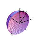
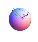
Figure 2: a) Foci and antipodal foci of the elliptic system of coordinates on ${\mathbb{S}}^{2}$. b) Distances from a point to the foci.

Given a point $P\in{\mathbb{S}}^{2}$, let us consider the distances $r_{1}\in[0,\pi R]$ and $r_{2}\in[0,\pi R]$ from $P$ to $F_{1}$ and $F_{2}$.

$$r_{1} = 2R\,\arcsin\sqrt{\frac{1}{2}\left(1-\cos\theta_{f}\,\cos\theta+\sin\theta_{f}\,\sin\theta\cos\varphi\right)}$$

$$r_{2} = 2R\,\arcsin\sqrt{\frac{1}{2}\left(1-\cos\theta_{f}\,\cos\theta-\sin\theta_{f}\,\sin\theta\cos\varphi\right)}\ ,$$

see Figure 2(b). The spherical elliptic coordinates of $P$ are half the sum and half the difference of $r_{1}$ and $r_{2}$: $2u=r_{1}+r_{2}$ , $2v=r_{1}-r_{2}$. $u\in(R\theta_{f},R(\pi-\theta_{f}))$, $v\in(-R\theta_{f},R\theta_{f})$. We remark that this version of elliptic coordinates in a sphere is equivalent to using conical coordinates constrained to ${\mathbb{S}}^{2}$, as defined e. g. in Reference MF . We shall use the abbreviated notation:

$$\mathop{\rm su}\nolimits = \sin\frac{u(t,x)}{R},\,\mathop{\rm sv}\nolimits=\sin\frac{v(t,x)}{R},\,\mathop{\rm sf}\nolimits=\sin\theta_{f}$$

$$\mathop{\rm su}\nolimits^{2} = \sin^{2}\frac{u(t,x)}{R}\,,\mathop{\rm sv}\nolimits^{2}=\sin^{2}\frac{v(t,x)}{R}\,,\mathop{\rm sf}\nolimits^{2}=\sin^{2}\theta_{f}\$$

and analogously for $\mathop{\rm cu}\nolimits$, $\mathop{\rm cv}\nolimits$, and $\mathop{\rm cf}\nolimits$. To pass from elliptical to Cartesian coordinates, or viceversa, one uses:

$$\phi_{1}(t,x) = {R\over\mathop{\rm sf}\nolimits}\mathop{\rm su}\nolimits\mathop{\rm sv}\nolimits\,\,\,,\quad\phi_{3}(t,x)={R\over\mathop{\rm cf}\nolimits}\mathop{\rm cu}\nolimits\mathop{\rm cv}\nolimits$$

$$\phi_{2}(t,x) = \pm\frac{R}{\mathop{\rm sf}\nolimits\mathop{\rm cf}\nolimits}\sqrt{(\mathop{\rm su}\nolimits^{2}-\mathop{\rm sf}\nolimits^{2})(\mathop{\rm sf}\nolimits^{2}-\mathop{\rm sv}\nolimits^{2})}\qquad,$$

whereas the differential arc-length reads:

$$ds^{2}_{{\mathbb{S}}^{2}}=\frac{\mathop{\rm su}\nolimits^{2}-\mathop{\rm sv}\nolimits^{2}}{\mathop{\rm su}\nolimits^{2}-\mathop{\rm sf}\nolimits^{2}}\cdot du^{2}+\frac{\mathop{\rm su}\nolimits^{2}-\mathop{\rm sv}\nolimits^{2}}{\mathop{\rm sf}\nolimits^{2}-\mathop{\rm sv}\nolimits^{2}}\cdot dv^{2}\qquad.$$

The spherical elliptic coordinates of the North and South Poles, and the foci are respectively: $(u_{N},v_{N})=(R\theta_{f},0)$, $(u_{S},v_{S})=(R(\pi-\theta_{f}),0)$, $(u_{F_{1}},v_{F_{1}})\equiv(R\theta_{f},-R\theta_{f})$, $(u_{F_{2}},v_{F_{2}})\equiv(R\theta_{f},R\theta_{f})$, $(u_{\bar{F}_{1}},v_{\bar{F}_{1}})\equiv(R(\pi-\theta_{f}),R\theta_{f})$, $(u_{\bar{F}_{2}},v_{\bar{F}_{2}})\equiv(R(\pi-\theta_{f}),-R\theta_{f})$.

V.2 Static field equations and Hamilton-Jacobi separability

We choose a system of spherical elliptic coordinates with the foci determined by $\theta_{f}=\arccos\sigma$, i.e., $\sigma^{2}={\rm cos}^{2}\theta_{f}$, $\bar{\sigma}^{2}={\rm sin}^{2}\theta_{f}$. We stress that the foci (and their antipodal points) are the branching points mentioned in the previous Section. In this coordinate system the action for the massive non-linear ${\mathbb{S}}^{2}$-sigma model reads:

$$S=\int dtdx\left\{\frac{1}{2}\left[\frac{\mathop{\rm su}\nolimits^{2}-\mathop{\rm sv}\nolimits^{2}}{\mathop{\rm su}\nolimits^{2}-\mathop{\rm sf}\nolimits^{2}}\partial_{\mu}u\partial^{\mu}u+\frac{\mathop{\rm su}\nolimits^{2}-\mathop{\rm sv}\nolimits^{2}}{\mathop{\rm sf}\nolimits^{2}-\mathop{\rm sv}\nolimits^{2}}\partial_{\mu}v\partial^{\mu}v\right]\right.$$

$$\hskip 56.9055pt\left.-V(u(t,x),v(t,x))\rule{0.0pt}{11.38092pt}\right\}\ ,$$

$$V(u,v)=\frac{R^{2}}{2(\mathop{\rm su}\nolimits^{2}-\mathop{\rm sv}\nolimits^{2})}\left[\mathop{\rm su}\nolimits^{2}(\mathop{\rm su}\nolimits^{2}-\mathop{\rm sf}\nolimits^{2})+\mathop{\rm sv}\nolimits^{2}(\mathop{\rm sf}\nolimits^{2}-\mathop{\rm sv}\nolimits^{2})\right]\,.$$

The static energy reads:

$$E[u,v]=\lambda\int dx\,{\cal E}(u^{\prime}(x),v^{\prime}(x),u(x),v(x))\ ,$$

$${\cal E}=\frac{1}{2}\left[\frac{\mathop{\rm su}\nolimits^{2}-\mathop{\rm sv}\nolimits^{2}}{\mathop{\rm su}\nolimits^{2}-\mathop{\rm sf}\nolimits^{2}}(u^{\prime})^{2}+\frac{\mathop{\rm su}\nolimits^{2}-\mathop{\rm sv}\nolimits^{2}}{\mathop{\rm sf}\nolimits^{2}-\mathop{\rm sv}\nolimits^{2}}(v^{\prime})^{2}\right]+V(u,v)\,\,.$$

Let us think of $E[u,v]$ as the action for a particle: ${\cal E}$ as the Lagrangian, $x$ as the time, $U(u,v)=-V(u,v)$ as the mechanical potential energy, and the target manifold ${\mathbb{S}}^{2}$ as the configuration space. The canonical momenta are: $p_{u}=\frac{\partial{\cal E}}{\partial u^{\prime}}$, $p_{v}=\frac{\partial{\cal E}}{\partial v^{\prime}}$, and the static field equations can be thought of as the Newtonian ODE’s:

$$\frac{d}{dx}\cdot\left(\frac{\mathop{\rm su}\nolimits^{2}-\mathop{\rm sv}\nolimits^{2}}{\mathop{\rm su}\nolimits^{2}-\mathop{\rm sf}\nolimits^{2}}\cdot u^{\prime}\right)=\frac{\delta V}{\delta u}$$

$$\frac{d}{dx}\cdot\left(\frac{\mathop{\rm su}\nolimits^{2}-\mathop{\rm sv}\nolimits^{2}}{\mathop{\rm sf}\nolimits^{2}-\mathop{\rm sv}\nolimits^{2}}\cdot v^{\prime}\right)=\frac{\delta V}{\delta v}\qquad.$$

Because the mechanical energy is

$$U(u,v) = -V(u,v)=-\frac{1}{\mathop{\rm su}\nolimits^{2}-\mathop{\rm sv}\nolimits^{2}}\,\left(f(u)+g(v)\right)=$$

$$= -\frac{R^{2}[\mathop{\rm su}\nolimits^{2}(\mathop{\rm su}\nolimits^{2}-\mathop{\rm sf}\nolimits^{2})+\mathop{\rm sv}\nolimits^{2}(\mathop{\rm sf}\nolimits^{2}-\mathop{\rm sv}\nolimits^{2})]}{2(\mathop{\rm su}\nolimits^{2}-\mathop{\rm sv}\nolimits^{2})}$$

this mechanical system is a Liouville type I integrable system, (see Per ). The Hamiltonian and the Hamilton-Jacobi equation of spherical Type I Liouville models have the form:

$$H=\frac{h_{u}+h_{v}}{\mathop{\rm su}\nolimits^{2}-\mathop{\rm sv}\nolimits^{2}}\,,\ \left\{\begin{array}[]{c}h_{u}=\frac{1}{2}(\mathop{\rm su}\nolimits^{2}-\mathop{\rm sf}\nolimits^{2})\,p_{u}^{2}-f(u)\\ h_{v}=\frac{1}{2}(\mathop{\rm sf}\nolimits^{2}-\mathop{\rm sv}\nolimits^{2})\,p_{v}^{2}-g(v)\end{array}\right.$$

$$\frac{\partial{\cal S}}{\partial x}+H\left(\frac{\partial{\cal S}}{\partial u},\frac{\partial{\cal S}}{\partial v},u,v\right)=0\ ,$$

which guarantees HJ separability in this system of coordinates. The separation ansatz ${\cal S}(x,u,v)$ $=-i_{1}x+{\cal S}_{u}(u)+{\cal S}_{v}(v)$ reduces the HJ equation to the two separated ODE’s, in the usual HJ procedure, leading to the complete solution: ${\cal S}={\cal S}(x,u,v,i_{1},i_{2})$:

$${\cal S} = -i_{1}x+{\rm sg}(p_{u})\int du\sqrt{\frac{2(\frac{i_{2}}{R^{2}}+i_{1}\mathop{\rm su}\nolimits^{2}+f(u))}{\mathop{\rm su}\nolimits^{2}-\mathop{\rm sf}\nolimits^{2}}}$$ (25)

$$+{\rm sg}(p_{v})\int dv\sqrt{\frac{2(-\frac{i_{2}}{R^{2}}-i_{1}\mathop{\rm sv}\nolimits^{2}+g(v))}{\mathop{\rm sf}\nolimits^{2}-\mathop{\rm sv}\nolimits^{2}}}$$

in terms of the mechanical energy $I_{1}=i_{1}$ and a second constant of motion: the separation constant $I_{2}=\frac{i_{2}}{R^{2}}$.

VI Non-topological kinks

We now identify the families of trajectories corresponding to the values $i_{1}=i_{2}=0$ of the two invariants in the mechanical system. These orbits are separatrices between bounded and unbounded motion in phase space and become solitary wave solutions in the field-theoretical model because the $i_{1}=i_{2}=0$ conditions force the boundary behavior (5). (See Ito and AAi for application of this idea to the search for solitary waves in other two-scalar field models with analogous mechanical systems which are HJ separable in elliptic coordinates.)

1. In a first step we find the Hamilton characteristic function for zero particle energy $(i_{1}=0=i_{2})$ by performing the integrations in (25): $W(u,v)={\cal S}_{u}(u,i_{1}=0,i_{2}=0)+{\cal S}_{v}(v,i_{1}=0,i_{2}=0)$,

$$W^{(\beta_{1},\beta_{2})}(u,v)=F^{(\beta_{1})}(u)+G^{(\beta_{2})}(v)$$

with $(-1)^{\beta_{1}}=-{\rm sg}\,p_{u}$, $(-1)^{\beta_{2}}=-{{\rm sg}\,p_{v}}\cdot{\rm sg}\,v$, and:

$$F^{(\beta_{1})}(u)=R^{2}(-1)^{\beta_{1}}\mathop{\rm cu}\nolimits\,,\quad G^{(\beta_{2})}(v)=R^{2}(-1)^{\beta_{2}}\mathop{\rm cv}\nolimits\,.$$

2. The HJ procedure provides the kink orbits by integrating ${\rm sg}\,p_{u}\int\frac{du}{(\mathop{\rm su}\nolimits^{2}-\mathop{\rm sf}\nolimits^{2})|\mathop{\rm su}\nolimits|}-{\rm sg}\,p_{v}\int\frac{dv}{(\mathop{\rm sf}\nolimits^{2}-\mathop{\rm sv}\nolimits^{2})|\mathop{\rm sv}\nolimits|}=R^{3}\gamma_{2}$:

$$e^{R^{2}\gamma_{2}\mathop{\rm sf}\nolimits^{2}} = \left[\frac{\left|\tan\frac{u-f}{2R}\tan\frac{u+f}{2R}\right|^{\frac{1}{2\mathop{\rm cf}\nolimits}}}{|\tan\frac{u}{2R}|}\right]^{{\rm sg}p_{u}}\cdot$$ (26)

$$\left[\frac{|\tan\frac{v}{2R}|}{\left|\tan\frac{v-f}{2R}\tan\frac{v+f}{2R}\right|^{\frac{1}{2\mathop{\rm cf}\nolimits}}}\right]^{{\rm sg}p_{v}}\ .$$

In Figure 3(a) a Mathematica plot is offered showing several orbits complying with (26) for several values of the integration constant $\gamma_{2}$. Note that all the orbits start and end at the North Pole and pass through the foci $\bar{F}_{1}$ such that we have shown a one-parametric family of non-topological kink orbits. In fact, there are four families of non-topological kinks among the solutions of (26): the orbits of a second family also start and end at the North Pole but pass through $\bar{F}_{2}$. The orbits in the second pair of NTK families start and end at the South Pole ant pass through either $F_{1}$ or $F_{2}$.

 

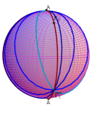
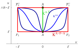
Figure 3: a) Several NTK kink orbits. b) The same NTK kink orbits in the elliptic rectangle.

Figure 4: NTK energy densities for three different values of $\gamma_{2}$: 1) $\gamma_{2}=-3$, highest peak on the left (blue) 2) $\gamma_{2}=0$, symmetrical peaks (green) 3) $\gamma_{2}=10$ highest peak on the right (red).

3. The HJ procedure requires similar integrations in ${\rm sg}\,p_{u}\int\frac{|\mathop{\rm su}\nolimits|du}{(\mathop{\rm su}\nolimits^{2}-\mathop{\rm sf}\nolimits^{2})}-{\rm sg}\,p_{v}\int\frac{|\mathop{\rm sv}\nolimits|dv}{(\mathop{\rm sf}\nolimits^{2}-\mathop{\rm sv}\nolimits^{2})}=R(x+\gamma_{1})$ to find the kink profiles (or particle “time ” schedules):

$$e^{2(x+\gamma_{1})\mathop{\rm cf}\nolimits}=\frac{\left|\tan\frac{u(x)-f}{2R}\tan\frac{u(x)+f}{2R}\right|^{{\rm sg}p_{u}}}{\left|\tan\frac{v(x)-f}{2R}\tan\frac{v(x)+f}{2R}\right|^{{\rm sg}p_{v}}}\qquad.$$ (27)

In Figure 4 the NTK energy densities for three values of $\gamma_{2}$ are plotted.

4. Reshuffling equations (26) and (27), it is possible to find the NTK families analytically, (28), based on $(u_{N},v_{N})=(R\theta_{f},0)$. The other families, based on $(u_{S},v_{S})=(R(\pi-\theta_{f}),0)$ are given by a similar formula.

$$\tan{u_{K}(x,\gamma_{1},\gamma_{2})\over 2R} = \frac{\pm\sqrt{2}\sqrt{1+e_{1}}e_{2}\mathop{\rm t\frac{f}{2}}\nolimits}{\sqrt{e_{1}+e_{2}^{2}+\mathop{\rm t\frac{f}{2}}\nolimits^{4}+e_{1}e_{2}^{2}\mathop{\rm t\frac{f}{2}}\nolimits^{4}-\sqrt{(e_{1}+e_{2}^{2}+\mathop{\rm t\frac{f}{2}}\nolimits^{4}+e_{1}e_{2}^{2}\mathop{\rm t\frac{f}{2}}\nolimits^{4})^{2}-4(1+e_{1})^{2}e_{2}^{2}\mathop{\rm t\frac{f}{2}}\nolimits^{4}}}}$$

$$\tan{v_{K}(x,\gamma_{1},\gamma_{2})\over 2R} = \frac{\pm\sqrt{e_{1}+e_{2}^{2}+\mathop{\rm t\frac{f}{2}}\nolimits^{4}+e_{1}e_{2}^{2}\mathop{\rm t\frac{f}{2}}\nolimits^{4}-\sqrt{(e_{1}+e_{2}^{2}+\mathop{\rm t\frac{f}{2}}\nolimits^{4}+e_{1}e_{2}^{2}\mathop{\rm t\frac{f}{2}}\nolimits^{4})^{2}-4(1+e_{1})^{2}e_{2}^{2}\mathop{\rm t\frac{f}{2}}\nolimits^{4}}}}{\sqrt{2}\sqrt{1+e_{1}}\mathop{\rm t\frac{f}{2}}\nolimits}$$ (28)

where we have used the new abbreviations: $e_{1}=e^{2(x+\gamma_{1})\mathop{\rm cf}\nolimits}\,\,\,,\,\,\,e_{2}=e^{x+\gamma_{1}-R^{2}\gamma_{2}\mathop{\rm sf}\nolimits^{2}}\,\,\,,\,\,\,\mathop{\rm t\frac{f}{2}}\nolimits=\tan\frac{f}{2R}$.

VII Non-topological kink instability: Morse index theorem

To study the (lack of) stability of NTK kinks, it is convenient to use the following notation for the elliptic variables: $u^{1}=u$, $u^{2}=v$. The static field equations read:

$$\frac{D}{dx}\cdot\frac{du^{i}}{dx}=g^{ij}\frac{d}{dx}\left(g_{jk}\frac{du^{k}}{dx}\right)=g^{ij}\frac{\partial V}{\partial u^{j}}\ .$$ (29)

Let us consider a one-parametric family of solutions of (29): $u^{i}_{K}(x;\gamma)$. The derivation of

$$\left(-\frac{D}{dx}\cdot\frac{du^{i}_{K}}{dx}+g^{ij}(u^{1}_{K},u^{2}_{K})\frac{\partial V}{\partial u^{j}}\right)\cdot g_{ik}\frac{\partial u^{k}_{K}}{\partial\gamma}=0$$

with respect to the parameter $\gamma$ implies:

$$\frac{D^{2}}{dx^{2}}\cdot\frac{\partial u^{i}_{K}}{\partial\gamma}+\frac{\partial u^{j}_{K}}{\partial x}\cdot\frac{\partial u^{k}_{K}}{\partial\gamma}\cdot\frac{\partial u^{l}_{K}}{\partial x}R^{i}_{jkl}+$$

$$+g^{ik}\left(\frac{\partial^{2}V}{\partial u^{j}\partial u^{k}}-\Gamma^{l}_{jk}(u^{1}_{K},u^{2}_{K})\frac{\partial V}{\partial u^{l}}\right)\frac{\partial u^{j}_{K}}{\partial\gamma}=0\,.$$

In the last three formulas the metric tensor, the covariant derivatives, the connection, the curvature tensor, and the gradient and Hessian of the potential are valued on $(u^{1}_{K},u^{2}_{K})$, see AMAJ2 . Thus, $\frac{\partial u^{i}_{K}}{\partial\gamma}$ is an eigenvector of the second order fluctuation operator of zero eigenvalue. The derivatives of the NTK solutions (28) with respect to the parameter $\gamma_{2}$ are accordingly eigenvectors of the second order fluctuation operator of zero eigenvalues orthogonal to the NTK orbit, i.e., Jacobi fields that move from one NTK kink to another with no cost in energy.

Better than direct derivation of (28) the Jabobi fields can be obtained from (26) and (27) by using implicit derivation with respect to the parameter $\gamma_{2}$ and solving the subsequent linear system. We skip the (deep) subtleties of this calculation and merely provide the explicit analytical expressions:

$$J^{\rm NTK}(x;\gamma_{2})=\frac{R^{3}(\mathop{\rm su}\nolimits^{2}-\mathop{\rm sf}\nolimits^{2})(\mathop{\rm sf}\nolimits^{2}-\mathop{\rm sv}\nolimits^{2})}{\mathop{\rm su}\nolimits^{2}-\mathop{\rm sv}\nolimits^{2}}\cdot$$

$$\hskip 28.45274pt\cdot\left({\rm sg}(p_{u})\,\mathop{\rm su}\nolimits\,\frac{\partial}{\partial u}\,-\,{\rm sg}(p_{v})\,\mathop{\rm sv}\nolimits\,\frac{\partial}{\partial v}\right)\ .$$ (30)

In Figures 5 a)-b), 6 a)-b) two Jacobi fields for two values of $\gamma_{2}$, as well as the corresponding NTK field profiles, are plotted for the three $\phi_{1}$, $\phi_{2}$, $\phi_{3}$ original field components.

 

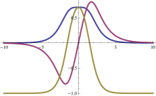
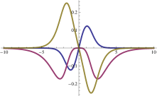
Figure 5: a) Profiles of the field components for NTK $\gamma_{2}=0$ kink. b) Plot of the Jacobi field $J^{NTK}(x;0)$

 

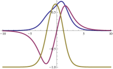
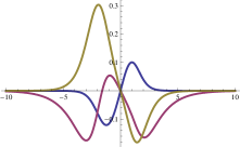
Figure 6: a) Profiles of the field components for NTK $\gamma_{2}=1$ kink. b) Plot of the Jacobi field $J^{NTK}(x;1)$

The zeroes of the Jacobi fields along a given $\gamma_{2}$-NTK orbit (in the four disconnected sectors) are as follows: either $A\equiv(u_{K}(-\infty;\gamma_{2})=f,v_{k}(-\infty;\gamma_{2})=0$), $\bar{F}_{1}\equiv(u_{K}(\bar{\gamma}_{1};\gamma_{2})=\pi R-f,v_{K}(\bar{\gamma}_{1};\gamma_{2})=-f$), $\bar{F}_{2}\equiv(u_{K}(\bar{\gamma}_{1};\gamma_{2})=\pi R-f,v_{K}(\bar{\gamma}_{1};\gamma_{2})=f$), or, $\bar{A}\equiv(u_{K}(-\infty;\gamma_{2})=\pi R-f,v_{k}(-\infty;\gamma_{2})=0$), $F_{1}\equiv(u_{K}(\bar{\gamma}_{1};\gamma_{2})=f,v_{K}(\bar{\gamma}_{1};\gamma_{2})=-f$), $F_{2}\equiv(u_{K}(\bar{\gamma}_{1};\gamma_{2})=f,v_{K}(\bar{\gamma}_{1};\gamma_{2})=f$). Thus, the conjugate points with respect to either the North or the South Poles along the NTK orbits are listed below:

$$\begin{array}[]{|c|c|c|}\hline\cr&&\\[-2.84544pt] {\bf Starting}\,{\bf Point}&{\bf Conjugate}\,{\bf Point}&{\bf Conjugate}\,{\bf Point}\\ \hline\cr&&\\[-2.84544pt] {\rm North}\,{\rm Pole}:A&{\rm Antipodal}\,{\rm Focus}:\bar{F}_{1}&{\rm Antipodal}\,{\rm Focus}:\bar{F}_{2}\\ \hline\cr&&\\[-2.84544pt] {\rm South}\,{\rm Pole}:\bar{A}&{\rm Focus}:F_{1}&{\rm Focus}:F_{2}\\ \hline\cr\end{array}$$

In this two-dimensional setting, the Morse index theorem states that the number of negative eigenvalues of the second order fluctuation operator around a given orbit is equal to the number of conjugate points crossed by the orbit ItoT . The reason is that the spectrum of the Schr$\ddot{\rm o}$dinger operator has in this case an eigenfunction with as many nodes as the Morse index, the Jacobi field, whereas the ground state has no nodes. The Jacobi fields of the NTK orbits cross one conjugate point, their Morse index is one, and the NTK kinks are unstable.

VIII Non-BPS non-topological kinks

The availability of the Hamilton characteristic function as a sum of one function of $u$ and another function of $v$ allows us to write the energy of static configurations á la Bogomolny:

$$E[u,v] = {\lambda\over 2}\int dx\left\{\frac{\mathop{\rm su}\nolimits^{2}-\mathop{\rm sv}\nolimits^{2}}{\mathop{\rm su}\nolimits^{2}-\mathop{\rm sf}\nolimits^{2}}\left(\frac{du}{dx}-\frac{\mathop{\rm su}\nolimits^{2}-\mathop{\rm sf}\nolimits^{2}}{\mathop{\rm su}\nolimits^{2}-\mathop{\rm su}\nolimits^{2}}\frac{dF^{(\beta_{1})}}{du}\right)^{2}\right.$$

$$+ \left.\frac{\mathop{\rm su}\nolimits^{2}-\mathop{\rm sv}\nolimits^{2}}{\mathop{\rm sf}\nolimits^{2}-\mathop{\rm sv}\nolimits^{2}}\left(\frac{dv}{dx}-\frac{\mathop{\rm sf}\nolimits^{2}-\mathop{\rm sv}\nolimits^{2}}{\mathop{\rm su}\nolimits^{2}-\mathop{\rm su}\nolimits^{2}}\frac{dG^{(\beta_{2})}}{dv}\right)^{2}\right\}$$

$$+ \lambda\int\,dx\,\frac{du}{dx}\frac{dF^{(\beta_{1})}}{du}+\lambda\int\,dx\,\frac{dv}{dx}\frac{dG^{(\beta_{2})}}{dv}\ .$$

Solutions of the first-order equations

$$\frac{du}{dx} \!=\! \frac{\mathop{\rm su}\nolimits^{2}-\mathop{\rm sf}\nolimits^{2}}{\mathop{\rm su}\nolimits^{2}-\mathop{\rm sv}\nolimits^{2}}\frac{dF^{(\beta_{1})}}{du}=-R(-1)^{\beta_{1}}\frac{\mathop{\rm su}\nolimits^{2}-\mathop{\rm sf}\nolimits^{2}}{\mathop{\rm su}\nolimits^{2}-\mathop{\rm sv}\nolimits^{2}}\mathop{\rm su}\nolimits$$ (31)

$$\frac{dv}{dx} \!=\! \frac{\mathop{\rm sf}\nolimits^{2}-\mathop{\rm sv}\nolimits^{2}}{\mathop{\rm su}\nolimits^{2}-\mathop{\rm sv}\nolimits^{2}}\frac{dG^{(\beta_{2})}}{dv}=-R(-1)^{\beta_{2}}\frac{\mathop{\rm sf}\nolimits^{2}-\mathop{\rm sv}\nolimits^{2}}{\mathop{\rm su}\nolimits^{2}-\mathop{\rm sv}\nolimits^{2}}\mathop{\rm sv}\nolimits$$ (32)

are absolute minima of the energy and therefore are stable. Note that the energy of the solutions of (31)-(32) is positive or zero because ${\rm sg}u^{\prime}={\rm sg}\frac{dF^{(\beta_{1})}}{du}$ and ${\rm sg}v^{\prime}={\rm sg}\frac{dG^{(\beta_{1})}}{dv}$.

Even though the NTK trajectories are solutions of the analogous mechanical system provided by the HJ procedure that is closely related to the ODE system (31)-(32), they do not strictly solve (31)-(32). Taking the quotient of the two equations in (31)-(32) we find the equation

$$\frac{du}{dv}=(-1)^{\beta_{1}-\beta_{2}}\frac{\mathop{\rm su}\nolimits^{2}-\mathop{\rm sf}\nolimits^{2}}{\mathop{\rm sf}\nolimits^{2}-\mathop{\rm sv}\nolimits^{2}}\,\frac{\mathop{\rm su}\nolimits}{\mathop{\rm sv}\nolimits}\qquad,$$ (33)

which determines the kink orbit flow. Note that this equation is identical to the equation in the HJ procedure that one must integrate to find (26). The subtle point, however, is that this flow is undefined, $\frac{0}{0}$, at the four foci: $F_{1}$, $F_{2}$, $\bar{F}_{1}$, $\bar{F}_{2}$, and all the NTK orbits pass through one of these dangerous points, see Figures 3(a) and 3(b). The non-topological kink orbits solve (31)-(32) for a given sign combination before meeting at a focus and are solutions of (31)-(32) with another choice of signs after leaving these orbit intersections. Thus, non-topological kinks are classified as non-BPS in the terminology of “pre-supersymmetric” systems. We remark that in elliptic coordinates the pathology is not in the Hamilton characteristic function but in the factors induced by the change to elliptic coordinates. The conclusion is that the energy of the NTK kinks must be computed piecewise along the orbit. $E_{K(\gamma_{2})}^{C}=2\lambda\left|G^{(\beta_{2})}(0)-G^{(\beta_{2})}(v^{\pm}_{B})\right|+2\lambda\left|F^{(\beta_{1})}(u^{+}_{B})-F^{(\beta_{1})}(u^{-}_{B})\right|$, i.e.,

$$E_{K(\gamma_{2})}^{C}=2\lambda R^{2}|1-\sigma|+2\lambda R^{2}|2\sigma|=2\lambda R^{2}(1+\sigma)$$ (34)

gives the kink energy as the action of the corresponding trajectory.

VIII.1 Singular $K_{1}$ and $K_{2}$ kinks: kink mass sum rule

Analysis of the BPS/non-BPS nature of the topological kinks in elliptic coordinates is illuminating. The $K_{1}/K_{1}^{*}$ kink orbits lie in the $v=0$ line, splitting the two-halves of the elliptic rectangle: $v_{K_{1}}=v_{K_{1}^{*}}=0$, see Figure 3(b). The first-order equations (31)-(32) on the $K_{1}/K_{1}^{*}$ kink orbits ($\beta_{1}=0$ gives kinks and $\beta_{1}=1$ anti-kinks) and the $K_{1}/K_{1}^{*}$ kink profiles in elliptic coordinates are:

$$\frac{du}{dx}=-(-1)^{\beta_{1}}R\frac{\mathop{\rm su}\nolimits^{2}-\mathop{\rm sf}\nolimits^{2}}{\mathop{\rm su}\nolimits}$$

$$u_{K_{1}}(x)=u_{K_{1}^{*}}(x)=R\arccos[\sigma\tanh((-1)^{\beta_{1}}\sigma x)]\ .$$

The $K_{1}/K_{1}^{*}$ kink energy saturates the BPS bound:

$$E_{K_{1}}^{C}=\lambda\left|F^{(\beta_{1})}(u_{K_{1}}(+\infty))-F^{(\beta_{1})}(u_{K_{1}}(-\infty))\right|=2\lambda R^{2}\sigma.$$

The $K_{2}/K_{2}^{*}$ kink orbits are the four edges of the elliptic rectangle: $u_{K_{2}}=u_{K_{2}^{*}}=R\theta_{f}$, $v_{K_{2}}=R\theta_{f}$, $v_{K_{2}}=-R\theta_{f}$, $u_{K_{2}}=u_{K_{2}^{*}}=R(\pi-\theta_{f})$, see again Figure 3(b). The $K_{2}/K_{2}^{*}$ kinks are accordingly three-step trajectories in the elliptic rectangle.

I. $-\infty<x<\log\tan{\theta_{f}\over 2}$ and $u_{K_{2}}^{I}=u_{K_{2}^{*}}^{I}=R(\pi-\theta_{f})$, the first-order ODE, and the solutions are:

$$\beta_{2}=1,\,v^{\prime}=R|\mathop{\rm sv}\nolimits|,\,v^{I}_{K_{2}}(x)=-v^{I}_{K_{2}^{*}}(x)=2R\arctan e^{x}\,.$$

II. $\log\tan{\theta_{f}\over 2}<x<\log\tan{\pi-\theta_{f}\over 2}$, $v_{K_{2}}^{II}=-v_{K_{2}^{*}}^{II}=R\theta_{f}$, the first-order ODE and the solution are:

$$\beta_{1}=0,\,u^{\prime}=-R\mathop{\rm su}\nolimits,\,u^{II}_{K_{2}}(x)=u^{II}_{K_{2}^{*}}(x)=2R\arctan e^{-x}\,.$$

III. $\log\tan{\pi-\theta_{f}\over 2}<x<+\infty$, $u_{K_{2}}^{III}=u_{K_{2}^{*}}^{III}$, the first-order equation and the solutions are:

$$\beta_{2}=0,\,v^{\prime}=-R|\mathop{\rm sv}\nolimits|,\,v^{III}_{K_{2}}(x)=-v^{III}_{K_{2}^{*}}(x)=2R\arctan e^{-x}\,.$$

Anti-kinks are obtained by changing the choices of $\beta_{1}$ and $\beta_{2}$. In any case, the $K_{2}/K_{2}^{*}$ kink energy is not of the BPS form:

$$E_{K_{2}}^{C}=\lambda\left|G^{(1)}(v(-\infty))-G^{(1)}(v(\log\tan\frac{\theta_{f}}{2}))\right|$$

$$+\lambda\left|F^{(0)}(u(\log{\rm tan}\frac{\theta_{f}}{2}))-F^{(0)}(u(\log{\rm cotan}\frac{\theta_{f}}{2}))\right|$$

$$+\lambda\left|G^{(0)}(v(\log{\rm cotan}\frac{\theta_{f}}{2}))-G^{(0)}(v(+\infty))\right|$$

$$=\lambda R^{2}|1-\mathop{\rm cf}\nolimits|+\lambda R^{2}|-2\mathop{\rm cf}\nolimits|+\lambda R^{2}|1-\mathop{\rm cf}\nolimits+1|=2\lambda R^{2}.$$

It is remarkable that these energies satisfy the following “Kink mass sum rule”:

$$E_{K(\gamma_{2})}^{C}=2\lambda R^{2}(1+\sigma)=E_{K_{2}}^{C}+E_{K_{1}}^{C}$$ (35)

In fact, the $|\gamma_{2}|\to\infty$ limit of the family of $K_{\gamma_{2}}$ (NTK) kinks is compatible with equation (26) only at the edges of the elliptic rectangle (forming the $K_{2}/K_{2}^{*}$ orbits) and the $K_{1}/K_{1}^{*}$ orbit. Therefore, the $K_{1}$ and $K_{2}$ form the boundary of the moduli space of $K_{\gamma_{2}}$ in such a way that (35) shows this combination as one of the NTK kinks.

IX Solitary spin waves

Field configurations that satisfy the Euler-Lagrange equations:

$$\frac{\partial A_{a}}{\partial t}(t,x)=\sum_{b=1}^{3}\,\left(\frac{\delta A_{b}}{\delta\phi_{a}}(t,x)-\frac{\delta A_{a}}{\delta\phi_{b}}(t,x)\right)\cdot\frac{\partial\phi_{b}}{\partial t}(t,x)$$

$$=\sum_{b=1}^{3}\,\sum_{c=1}^{3}\,\varepsilon_{abc}B_{c}[\Phi(t,x)]\cdot\frac{\partial\phi_{b}}{\partial t}(t,x)$$

are extremals of the “Wess-Zumino” action:

$$S_{\rm WZ}[\Phi]=R^{2}\int\,dtdx\,\sum_{a=1}^{3}\,A_{a}[\Phi(t,x)]\frac{\partial\phi_{a}}{\partial t}(t,x)\qquad\qquad.$$

In particular a “magnetic monopole ” field $B_{a}[\Phi(t,x)]=\frac{\phi_{a}(t,x)}{R^{3}}$ in the ${\mathbb{R}}^{3}$ internal space where the ${\mathbb{S}}^{2}$-sphere is embedded is obtained by the choice of singular “vector potentials”:

$$A_{1}^{\pm}[\Phi(t,x)] = -\frac{\phi_{2}}{\sqrt{\phi_{1}^{2}+\phi_{2}^{2}+\phi_{3}^{2}}(\phi_{3}\pm\sqrt{\phi_{1}^{2}+\phi_{2}^{2}+\phi_{3}^{2}})}$$

$$A_{2}^{\pm}[\Phi(t,x)] = \frac{\phi_{1}}{\sqrt{\phi_{1}^{2}+\phi_{2}^{2}+\phi_{3}^{2}}(\phi_{3}\pm\sqrt{\phi_{1}^{2}+\phi_{2}^{2}+\phi_{3}^{2}})}$$

$$A_{3}^{\pm}[\Phi(t,x)] = 0\qquad\qquad.$$

$\vec{A}^{+}[\Phi(t,x)]]$ is singular on the negative $\phi_{3}$-axis but a gauge transformation to $\vec{A}^{-}[\Phi(t,x)]]$ moves the Dirac string -henceforth a gauge artifact- to the positive $\phi_{3}$-axis. The scalar fields are constrained to live in the $\phi_{1}^{2}(t,x)+\phi_{2}^{2}(t,x)+\phi_{3}^{2}(t,x)=R^{2}$ sphere, a surface where this magnetic flux is constant. Therefore, Stoke’s theorem tells us that $S_{\rm WZ}=R^{2}\int\,dx\,\oint\,\sum_{a=1}^{3}d\phi_{a}(x)A_{a}[\Phi(x)]$ is the area bounded by a closed curve in ${\mathbb{S}}^{2}$.

The important point is that the Euler-Lagrange equations for the sum of the two actions $S_{\rm WZ}+S$, where $S$ is the action of our model, are:

$${1\over R}\sum_{b=1}^{3}\,\sum_{c=1}^{3}\,\varepsilon_{abc}\phi_{c}\frac{\partial\phi_{b}}{\partial t}+\Box\phi_{a}+\frac{\alpha_{a}^{2}}{\lambda^{2}}\phi_{a}=0\ .$$ (36)

At the long wavelength limit, the ODE system (36) become the Landau-Lifshitz system of equations of ferromagnetism. The connection between the semi-classical (high-spin) limit of the Heisenberg model and the quantum non-linear ${\mathbb{S}}^{2}$-sigma model is well established Hal .

IX.1 Spin waves

Plugging the constraint into (36), we find the system of two ODE’s:

$$- \sum_{\alpha}\varepsilon_{\alpha\beta}\frac{{\rm sg}\phi_{3}}{R}\left(\sqrt{R^{2}-\sum_{\gamma}\phi_{\gamma}\phi_{\gamma}}\cdot\frac{\partial\phi_{\alpha}}{\partial t}\right.$$ (37)

$$\left.+\phi_{\alpha}\frac{\sum_{\gamma}\phi_{\gamma}\partial_{t}\phi_{\gamma}}{\sqrt{R^{2}-\sum_{\gamma}\phi_{\gamma}\phi_{\gamma}}}\right)+\Box\phi_{\beta}+m_{\beta}^{2}\phi_{\beta}$$

$$+ \frac{\phi_{\beta}}{R^{2}-\sum_{\gamma}\phi_{\gamma}\phi_{\gamma}}\left[\frac{\sum_{\gamma}\phi_{\gamma}\partial^{\mu}\phi_{\gamma}+\sum_{\delta}\phi_{\delta}\partial_{\mu}\phi_{\delta}}{R^{2}-\sum_{\gamma}\phi_{\gamma}\phi_{\gamma}}\right.$$

$$\left.-\sum_{\gamma}\left(\partial^{\mu}\phi_{\gamma}\partial_{\mu}\phi_{\gamma}+\phi_{\gamma}\Box\phi_{\gamma}\right)\right]=0\ .$$

$\alpha,\beta,\gamma=1,2$, $m_{1}^{2}=1$, $m_{2}^{2}=\sigma^{2}$. The ground states are the homogeneous solutions of this system: $\phi_{1}^{0}=\phi_{2}^{0}=0$, $\phi_{3}^{0}=\pm R$. In order to visualize these configurations in, e. g., Figure 7 we draw the spin chain in such a way that the $\phi_{2}:\phi_{3}$ plane is perpendicular to the $x$ spatial line whereas $\phi_{1}$ is aligned with the $x$-axis. We stress that this choice of basis is arbitrary but it is easy to figure out the formulas and the graphics in another rotated basis for the magnetization vector: $\vec{\phi}(x)=\phi_{1}(x)\vec{e}_{1}+\phi_{2}(x)\vec{e}_{2}+\phi_{3}(x)\vec{e}_{3}=\phi_{1}^{\prime}(x)\vec{e^{\prime}}_{1}+\phi_{2}^{\prime}(x)\vec{e^{\prime}}_{2}+\phi_{3}^{\prime}(x)\vec{e^{\prime}}_{3}$. The main features of our preferred basis $\vec{e}_{1},\vec{e}_{2},\vec{e}_{3}$ are: 1) The $\vec{e}_{1}$ vector points in the direction of weaker $-V(\theta,\varphi)$ potential, see Figure 1(b). 2) $\vec{e}_{1},\vec{e}_{2},\vec{e}_{3}$ is the basis used in the continuous XY (in fact YZ) model of easy-axis ferromagnets near the Curie point, see BW ; BWZ and References quoted therein.

  

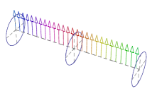
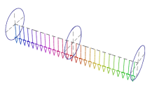
Figure 7: a) Ground state $\phi_{3}^{0}=R$ . All the spins are aligned pointing to the North Pole b) Ground state $\phi_{3}^{0}=-R$. All the spins are aligned pointing to the South Pole.

The spin fluctuations $\phi_{1}(t,x)=\delta\phi_{1}(t,x)$, $\phi_{2}(t,x)=\delta\phi_{2}(t,x)$ around the ground state $\phi_{3}(t,x)=R$ satisfy the linearized equations:

$$0 = \frac{\partial\delta\phi_{2}}{\partial t}+\frac{\partial^{2}\delta\phi_{1}}{\partial t^{2}}-\frac{\partial^{2}\delta\phi_{1}}{\partial x^{2}}+\delta\phi_{1}$$

$$0 = -\frac{\partial\delta\phi_{1}}{\partial t}+\frac{\partial^{2}\delta\phi_{2}}{\partial t^{2}}-\frac{\partial^{2}\delta\phi_{2}}{\partial x^{2}}+\sigma^{2}\delta\phi_{2}^{2}\,.$$

Therefore, the spin waves:

$$\delta\phi_{\alpha}(t,x) = {1\over\sqrt{\lambda L}}\sum_{k}\,{1\over\sqrt{\omega(k)}}\left(a_{\alpha}(k)e^{i\omega t-ikx}+\right.$$ (38)

$$\left.+a_{\alpha}^{*}(k)e^{-i\omega t+ikx}\right)$$

satisfying periodic boundary conditions $\delta\phi_{\alpha}(t,x)=\delta\phi_{\alpha}(t,x+\lambda L)$ are solutions of (38) for the frequencies complying with the homogeneous system of algebraic equations:

$$\left(\begin{array}[]{cc}-\omega^{2}+k^{2}+1&i\omega\\ -i\omega&-\omega^{2}+k^{2}+\sigma^{2}\end{array}\right)\left(\begin{array}[]{c}a_{1}(k)\\ a_{2}(k)\end{array}\right)=\left(\begin{array}[]{c}0\\ 0\end{array}\right)\,.$$ (39)

At the long wavelength limit $\omega^{2}<<\omega$, (39) is tantamount to the non-relativistic dispersion law

$$\omega^{2}(k^{2})=(k^{2}+1)(k^{2}+\sigma^{2})$$

characteristic of ferromagnetic materials, although the quadratic terms in the free energy prevent the standard $\omega(k)=k^{2}$ form.

IX.2 Bloch and Ising walls

One may check that the $K_{1}/K_{1}^{*}$ kinks (11) solve the static Landau-Lifshitz equations (37) on the $\phi_{1}=0$ orbit:

$$\frac{d^{2}\phi_{2}}{dx^{2}}=\frac{-\phi_{2}}{R^{2}-\phi_{2}^{2}}\left[\frac{(\phi_{2}\frac{d\phi_{2}}{dx})^{2}}{R^{2}-\phi_{2}^{2}}+\left(\frac{d\phi_{2}}{dx}\right)^{2}+\phi_{2}\frac{d^{2}\phi_{2}}{dx^{2}}\right]+\sigma^{2}\phi_{2}$$

The $K_{1}/K_{1}^{*}$ kinks of the non-linear sigma model are consequently solitary spin waves of this non-relativistic system, see Figure 8.

 

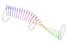
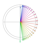
Figure 8: Graphic arrow representation of the $K_{1}$ kinks: a) $K_{1}$ spin chain. b) Perspective from one component of the boundary of ${\mathbb{S}}^{2}\times{\mathbb{R}}$ showing how the spin flip happens by means of a $\pi$-rotation around the $\phi_{1}$-axis.

Simili modo, the $K_{2}/K_{2}^{*}$ kinks (12) solve (37) along the $\phi_{2}=0$ kink orbit:

$$\frac{d^{2}\phi_{1}}{dx^{2}}=\frac{-\phi_{1}}{R^{2}-\phi_{1}^{2}}\left[\frac{(\phi_{1}\frac{d\phi_{1}}{dx})^{2}}{R^{2}-\phi_{1}^{2}}+\left(\frac{d\phi_{1}}{dx}\right)^{2}+\phi_{1}\frac{d^{2}\phi_{1}}{dx^{2}}\right]+\phi_{1}$$

and are also spin solitary waves in this system, (Fig. 9).

 

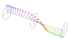
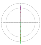
Figure 9: Graphic arrow representation of the $K_{2}$ kink a) $K_{2}$ spin chain. b) Perspective from one component of the boundary of ${\mathbb{S}}^{2}\times{\mathbb{R}}$ showing a forward spin flip.

Because the system of ODE’s giving static solutions of the (36) PDE system is the same as the static field equations of the non-linear ${\mathbb{S}}^{2}$-sigma model, the NTK kinks are also solitary spin waves, see Figure 10.

 

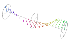
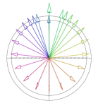
Figure 10: Graphic arrow representation of $K_{\gamma_{2}}$ kinks: a) $K_{\gamma_{2}}$ spin chain. b) Perspective from the boundary of ${\mathbb{S}}^{2}\times{\mathbb{R}}$ showing the $2\pi$ rotation around the $\phi_{1}$-axis of the spin to come back to the initial ground state.

In sum, understood as solitary spin waves $K_{1}/K_{1}^{*}$ kinks are Bloch walls whereas $K_{2}/K_{2}^{*}$ kinks are Ising walls describing interfaces between ferromagnetic domains, see BW , BWZ . In this model we have thus found a moduli space of solitary waves with an structure very similar to the structure of the space of solitary waves of the XY model described in References BW and BW1 . There are Bloch and Ising walls and a one-parametric family of NTK kinks that are non-linear superpositions of one Bloch and one Ising wall with arbitrary separation between their centers. The novelties here are: a) there is no need in the free energy of fourth-order terms in the magnetization in the non-linear sigma model for finding these mixtures of Bloch and Ising walls. b) The analytical expressions (28) differ from their analogues in the XY model.

From the stability analysis performed in previous Sections, it is clear that only the Bloch walls are stable and saturate the Bogomolny bound. Things are different at the $\sigma=1$ limit where all the kinks are topological, Bloch walls, and saturate the Bogomolny bound. In this latter case the structure of the kink space is akin to the kink space structure of the BNRT model BNRT , see SV , AMAJ1 , SAH . There is a one-parametric family of degenerate Bloch walls saturating the Bogomolny bound.

X Further comments: supersymmetry and stability

Finally, we briefly explore the possibility of embedding our bosonic model with its moduli space of kinks in a broader supersymmetric framework. It turns out that the simpler ${\cal N}=1$, ${\it d}=1+1$ SUSY version of the massive non-linear ${\mathbb{S}}^{2}$-sigma model only exists if the masses of the pseudo Nambu-Goldstone bosons are equal ($\sigma=1$). It also seems difficult to build more exotic possibilities coming from dimensional reduction of models of Kahler or hyper-Kahler nature because the potential energy density is not compatible with complex structures when $\sigma\neq 1$.

X.1 Isothermal coordinates

It is convenient to introduce isothermal coordinates in the chart ${\mathbb{S}}^{2}-\{(0,0,-R)\}$, which are obtained via stereographic projection from the South Pole:

$$\chi^{1} = \frac{\phi_{1}}{1+\frac{\phi_{3}}{R}}=\frac{R\phi_{1}}{R+{\rm sg}(\phi_{3})\sqrt{R^{2}-\phi_{1}^{2}-\phi_{2}^{2}}}$$

$$\chi^{2} = \frac{\phi_{2}}{1+\frac{\phi_{3}}{R}}=\frac{R\phi_{2}}{R+{\rm sg}(\phi_{3})\sqrt{R^{2}-\phi_{1}^{2}-\phi_{2}^{2}}}\,.$$ (40)

The metric and the action in this coordinate system read:

$$ds^{2}=\frac{4R^{4}}{(R^{2}+\chi^{1}\chi^{1}+\chi^{2}\chi^{2})^{2}}(d\chi^{1}d\chi^{1}+d\chi^{2}d\chi^{2})$$

$$S[\chi^{1},\chi^{2}]=\int\,dx^{2}\,\frac{2R^{4}}{(R^{2}+\chi^{1}\chi^{1}+\chi^{2}\chi^{2})^{2}}\cdot\left[\partial_{\mu}\chi^{1}\partial^{\mu}\chi^{1}+\right.$$

$$\left.+\partial_{\mu}\chi^{2}\partial^{\mu}\chi^{2}-(\chi^{1}\chi^{1}+\sigma^{2}\chi^{2}\chi^{2})\right]\ ,$$

whereas the $K_{1}$ kinks are given by:

$$\chi^{1}_{K_{1}}(x)=0\,,\ \chi^{2}_{K_{1}}(x)=\pm R\,\,{\rm exp}[\pm\sigma(x-x_{0})]\ ,$$ (41)

and we rewrite the second order fluctuation operator around the $K_{1}$ kink (with $\chi_{K_{1}}^{2}(x)=Re^{-\sigma x})$) in the form:

$$\Delta_{K_{1}}\eta=-\left(\frac{d^{2}\eta^{1}}{dx^{2}}+2\sigma(1-{\rm tanh}\sigma x)\frac{d\eta^{1}}{dx}\right.$$

$$\left.-\left(1-2\sigma^{2}+2\sigma^{2}\tanh\sigma x\right)\eta^{1}\right)\frac{\partial}{\partial\chi^{1}}-\left(\frac{d^{2}\eta^{2}}{dx^{2}}+\right.$$

$$\left.+2\sigma(1-\tanh\sigma x)\frac{d\eta^{2}}{dx}+\sigma^{2}\left(1-2\tanh\sigma x\right)\eta^{2}\right)\frac{\partial}{\partial\chi^{2}}\ .$$

In a parallel frame $\mu=\mu^{1}(x)\frac{\partial}{\partial\chi^{1}}+\mu^{2}(x)\frac{\partial}{\partial\chi^{2}}\in\Gamma(T{\mathbb{S}}^{2}\left|{}_{K_{1}})\right.$, $\frac{d\mu^{i}}{dx}+\Gamma^{i}_{jk}(\chi_{K})\chi_{K}^{\prime j}\mu^{k}=0$, along the $K_{1}$ kink:

$$\frac{d\mu^{1}}{dx}+\sigma(1-\tanh)\mu^{1}(x)=0\,\Rightarrow\,\mu^{1}(x)=1+e^{-2\sigma x}$$

$$\frac{d\mu^{2}}{dx}+\sigma(1-\tanh)\mu^{2}(x)=0\,\Rightarrow\,\mu^{2}(x)=1+e^{-2\sigma x}\ .$$

we recover the P$\ddot{\rm o}$sch-Teller operators:

$$\Delta_{K_{1}}\eta=\left(-\frac{d^{2}\eta^{1}}{dx^{2}}+(1-\frac{2\sigma^{2}}{{\rm cosh}^{2}\sigma x})\eta^{1}\right)\,(1+e^{-2\sigma x})\frac{\partial}{\partial\chi^{1}}$$

$$+\left(-\frac{d^{2}\eta^{2}}{dx^{2}}+(\sigma^{2}-\frac{2\sigma^{2}}{{\rm cosh}^{2}\sigma x})\eta^{2}\right)\,(1+e^{-2\sigma x})\frac{\partial}{\partial\chi^{2}}$$ (42)

Note that now the $K_{1}$ orbits are the positive and negative ordinate half-axes, the stereographic projections of the $\varphi=\frac{\pi}{2}$ and $\varphi=\frac{3\pi}{2}$ half-meridians, such that fluctuations orthogonal to the orbit run in the direction of the abscissa axis.

X.2 The ${\cal N}=1$ massive SUSY sigma model

In Reference AGMT we analyzed the relationship of the complete solution of the Hamilton-Jacobi equation for zero energy and the superpotential of a supersymetric associated classical mechanical system. Thus, we are tempted to use the Hamilton characteristic function

$$W^{(\beta_{1},\beta_{2})}(\chi)=\frac{(-1)^{\beta_{1}}R^{2}}{R^{2}+\chi^{1}\chi^{1}+\chi^{2}\chi^{2}}\cdot$$ (43)

$$\sqrt{\left(\sigma_{+}(\beta_{2})R^{2}+\sigma_{-}(\beta_{2})(\chi^{1}\chi^{1}+\chi^{2}\chi^{2})\right)^{2}-4\bar{\sigma}^{2}R^{2}\chi^{1}\chi^{1}},$$

$\sigma_{\pm}(\beta_{2})=1\pm(-1)^{\beta_{2}}\sigma$, to build the ${\cal N}=1$ SUSY extension of our massive non-linear ${\mathbb{S}}^{2}$-sigma model. On one hand we have that:

$$\frac{1}{2}g^{ij}\frac{\partial W^{(\beta_{1},\beta_{2})}}{\partial\chi^{i}}\cdot\frac{\partial W^{(\beta_{1},\beta_{2})}}{\partial\chi^{j}}=\frac{2R^{2}(\chi^{1}\chi^{1}+\sigma^{2}\chi^{2}\chi^{2})}{(R^{2}+\chi^{1}\chi^{1}+\chi^{2}\chi^{2})^{2}}\ ,$$

$\forall\beta_{1},\beta_{2}$. On the other hand (43) is free of branch points only for $\sigma=1$. Supersymmetry does not allow superpotentials with branch points and it seems that Hamilton-Jacobi characteristic functions are compatible with a weaker form called pseudo-supersymmetry in PT . We close our eyes to this fact for a moment and proceed to formally build the ${\cal N}=1$ SUSY extension of our model using (43).

There are also two Majorana spinor fields:

$$\psi^{i}(x^{\mu})=\left(\begin{array}[]{c}\psi_{1}^{i}(x^{\mu})\\ \psi_{2}^{i}(x^{\mu})\end{array}\right)\,,\,(\psi_{\alpha}^{i})^{*}=\psi_{\alpha}^{i},\ \alpha=1,2\,.$$

We choose the Majorana representation $\gamma^{0}=\sigma^{2},\gamma^{1}=i\sigma^{1},\gamma^{5}=\sigma^{3}$ of the Clifford algebra $\{\gamma^{\mu},\gamma^{\nu}\}=2g^{\mu\nu}$ and define the Majorana adjoints as: $\bar{\psi}^{i}=(\psi^{i})^{t}\gamma^{0}$. The action of the supersymmetric model is:

$$S=\int\frac{dx^{2}}{2}\left\{g_{ij}\left(\partial_{\mu}\chi^{i}\partial^{\mu}\chi^{j}+i\bar{\psi}^{i}\gamma^{\mu}(\partial_{\mu}\psi^{j}+\Gamma^{j}_{lk}\partial_{\mu}\chi^{k}\psi^{l})\right)\right.$$

$$\left.-\frac{1}{6}R_{ijlk}\bar{\psi}^{i}\psi^{j}\bar{\psi}^{l}\psi^{k}-g^{ij}\frac{\partial W}{\partial\chi^{i}}\frac{\partial W}{\partial\chi^{j}}-\bar{\psi}^{i}\frac{D\partial W}{\partial\chi^{i}\partial\chi^{j}}\psi^{j}\right\}\,\,,$$

where $\frac{D\partial W}{\partial\chi^{i}\partial\chi^{j}}=\frac{\partial^{2}}{\partial\chi^{i}\partial\chi^{j}}+\Gamma^{k}_{ij}\frac{\partial W}{\partial\chi^{k}}$. The spinor supercharge

$$Q=\int\,dx\,g_{ij}\left(\gamma^{\mu}\gamma^{0}\psi^{i}\partial_{\mu}\chi^{j}+i\gamma^{0}\psi^{i}g^{jk}\frac{\partial W}{\partial\chi^{k}}\right)$$ (44)

acts on the configuration space and leaves the action invariant. Time-independent finite energy configurations complying with

$$\frac{d\chi^{i}}{dx}=g^{ij}\frac{\partial W}{\partial\chi^{j}}\ ,\ \psi^{i}_{1}(x)=-\psi^{i}_{2}(x)$$ (45)

annihilates the supercharge combination $Q_{1}+Q_{2}$ and these solutions might be interpreted as $\frac{1}{2}$ BPS states in this supersymmetric framework. In particular, the SUSY $K_{1}$ kinks

$$\chi^{1}_{K_{1}}(x)=0 \chi^{2}_{K_{1}}=\pm Re^{\pm\sigma x}$$ ,

$$\psi^{1}_{K_{1}}(x)=\left(\begin{array}[]{c}0\\ 0\end{array}\right) \psi^{2}_{K_{1}}(x)=\pm\sigma Re^{\pm\sigma x}\left(\begin{array}[]{c}1\\ -1\end{array}\right)$$ ,

satisfy (45) (with appropriate choices of $\beta_{1}$, $\beta_{2}$). Note that $\psi^{2}_{K_{1}}(x)$ is the SUSY partner of $\chi^{2}_{K_{1}}(x)$ under the action of the broken SUSY supercharge $Q_{1}-Q_{2}$. We also remark that

$$\frac{d\chi^{2}_{K_{1}}}{dx}=\pm\sigma Re^{\pm\sigma x}=\pm\sigma R(1+e^{\pm 2\sigma x})\cdot\frac{1}{\cosh\sigma x}\ ,$$

i.e., the fermionic partner in the SUSY kink is the zero mode of the second order fluctuation operator back from the parallel frame to the $K_{1}$ orbit.

X.3 Fermionic fluctuations

The Dirac equation ruling the small fermionic fluctuations on the $K_{1}$ kink reads:

$$D\delta\psi^{i}(t,x) = i(\gamma^{0}\partial_{0}-\gamma^{1}\partial_{1})\delta\psi^{i}(t,x)$$ (47)

$$-i\gamma^{1}\Gamma^{i}_{jk}(\chi_{K_{1}})\partial_{1}\chi^{j}_{K_{1}}(x)\delta\psi^{k}(t,x)$$

$$+g^{ij}(\chi_{K_{1}})\frac{D\partial W}{\partial\chi^{j}\partial\chi^{k}}(\chi_{K_{1}})\delta\psi^{k}(t,x)\quad.$$

Acting on (47) with the adjoint Dirac operator, the search for solutions of $D^{\dagger}D\delta\psi^{i}(t,x)=0$ of the stationary form $\delta\psi^{i}(t,x)=e^{i\omega t}\delta\varrho^{i}(x,\omega)$ requires us to deal with the following ODE system:

$$-\frac{d^{2}}{dx^{2}}\delta\varrho^{i}(x)+g^{ij}\frac{D\partial W}{\partial\chi^{j}\partial\chi^{k}}\cdot g^{kl}\frac{D\partial W}{\partial\chi^{l}\partial\chi^{m}}\delta\varrho^{m}(x)$$

$$+R^{i}_{jkl}\frac{d}{dx}\chi^{j}_{K_{1}}\frac{d}{dx}\chi^{k}_{K_{1}}\delta\varrho^{l}(x)$$

$$-i\gamma^{1}g^{ij}\frac{\partial W}{\partial\chi^{j}}\cdot g^{kl}\frac{D^{2}\partial W}{\partial\chi^{k}\partial\chi^{l}\partial\chi^{m}}\delta\varrho^{m}(x)=\omega^{2}\delta\varrho^{i}(x)$$

valued at $\chi=\chi_{K_{1}}$.

On eigenspinors of $-i\gamma^{1}=\sigma^{1}$, $\delta\varrho^{i}_{1}(x)=\pm\delta\varrho^{i}_{2}(x)=\delta\varrho^{i}_{\pm}(x)$, the above spectral ODE system reduce to the (symbolically written) pair of equations:

$$\bigtriangleup^{\pm}_{K_{1}}\delta\varrho_{\pm}=\left[-\frac{d^{2}}{dx^{2}}+W^{\prime\prime}\otimes W^{\prime\prime}+R\pm W^{\prime}\otimes W^{\prime\prime\prime}\right]\delta\varrho_{\pm}\ .$$ (48)

$\bigtriangleup^{+}_{K_{1}}$ is exactly equal to the second order differential operator ruling the bosonic fluctuations. Therefore, in the parallel frame to the $K_{1}$ orbit we write $\bigtriangleup^{+}_{K_{1}}$ in matrix form:

$$\bigtriangleup^{+}_{K_{1}}=\left(\begin{array}[]{cc}-\frac{d^{2}}{dx^{2}}+1-\frac{2\sigma^{2}}{{\rm cosh}^{2}\sigma x}&0\\ 0&-\frac{d^{2}}{dx^{2}}+\sigma^{2}-\frac{2\sigma^{2}}{{\rm cosh}^{2}\sigma x}\end{array}\right)\,.$$

In the same frame $\bigtriangleup^{-}_{K_{1}}$ is the intertwined partner, see MRNW :

$$\bigtriangleup^{-}_{K_{1}}=\left(\begin{array}[]{cc}-\frac{d^{2}}{dx^{2}}+1&0\\ 0&-\frac{d^{2}}{dx^{2}}+\sigma^{2}\end{array}\right)\,.$$

If $\sigma\neq 1$, there is a bound state in $\bigtriangleup^{+}_{K_{1}}$ of energy $1-\sigma^{2}$ unpaired with an eigenstate of the same energy in $\bigtriangleup^{-}_{K_{1}}$, a fact incompatible with supersymmetry as we expected from the use of the complete solution of the Hamilton-Jacobi equation as superpotential, closing our eyes to the fact that, related to the instability of $NTK$ and $K_{2}$ kinks, the Hamilton characteristic function has branching points at the foci defining the elliptic coordinate system. A similar problem arouse in ABGLM1 and ABGLM2 where meromorphic Hamilton characteristic functions have been found. It is an open problem to explore whether or not these milder singularities allow the use of these Hamilton characteristic functions as superpotentials to extend the bosonic models dealt with in ABGLM1 , ABGLM2 to the supersymmetric framework.

If the masses are equal ($\sigma=1$), however, the Hamilton characteristic function is free of branching points and the unpaired states are zero modes. The ${\cal N}=1$ SUSY model is correct and we can apply the SUSY version of the Cahill-Comtet-Glauber formula proposed in BC1 to find the same one-loop correction to the SUSY ${\mathbb{S}}^{2}$ kink as given in MRNW :

$$\bigtriangleup E_{K_{1}}^{\rm SUSY}(\sigma=1)=-\frac{\lambda}{2\pi}\sum_{i=1}^{2}(\sin\nu_{i}^{+}-\nu_{i}^{+}\cos\nu_{i}^{+})=-\frac{\lambda}{\pi}\,\,.$$

Here $\nu_{1}^{+}=\nu_{2}^{+}=\arccos(0)=\frac{\pi}{2}$ are the angles obtained from the bound states of $\bigtriangleup_{K_{1}}^{+}$. There are no bound states in the spectrum of $\bigtriangleup_{K_{1}}^{-}$.

XI Acknowledgements

We are grateful to M. Santander, S. Woodford, I. Barashenkov, M. Nitta, P. Letelier, D. Bazeia, and Y. Fedorov for informative and illuminating electronic/ordinary mail correspondence and/or oral conversations on several issues concerning this work. Any misunderstanding is the authors’s own responsibility.

We also thank the Spanish Ministerio de Educacion y Ciencia and Junta de Castilla y Leon for partial support under grants FIS2006-09417 and GR224.

References

- (1) A. Alonso Izquierdo, M. A. Gonzalez Leon, and J. Mateos Guilarte, Phys. Rev. Lett. 101 (2008) 131602
- (2) K. Cahill, A. Comtet, and R. Glauber, Phys. Lett. 64B(1976) 283-285
- (3) E. R. C. Abraham and P. K. Townsend, Phys. Lett. B291 (1992) 85-88
- (4) E. R. C. Abraham and P. K. Townsend, Phys. Lett. B295 (1992) 225-232
- (5) M. Arai, M. Naganuma, M. Nitta, and N. Sakai, Nucl. Phys. B652 (2002) 35-71
- (6) N. Dorey, JHEP 9811 (1998) 005
- (7) R. A. Leese, Nucl. Phys. B366 (1991) 283-314
- (8) E. Abraham, Phys. Lett. B278 (1992) 291-296
- (9) J. P. Gauntlet, R. Portugues, D. Tong, P. K. Townsend, Phys. Rev. D63 (2001) 085002
- (10) Y. Isozumi, M. Nitta, K. Oshasi, N. Sakai, Phys. Rev. D71 (2005) 065018
- (11) M. Eto, Y. Isozumi, M. Nitta, K. Oshasi, N. Sakai, Jour. Phys. A39 (2006) R315-R392
- (12) M. Eto, and N. Sakai, Phys. Rev. D68 (2003) 125001
- (13) D. Bazeia, and A. R. Gomes, JHEP 05(2004) 012
- (14) A. de Souza Dutra, A. C. Amaro de Faria, and M. Holt, Phys. Rev. D78(2008) 043526
- (15) S. F. Coleman, Comm. Math. Phys. 31 (1973) 259
- (16) S. F. Coleman, “Aspects of symmetry”, Cambridge University Press, 1985, Chapter 6: “Classical lumps and their quantum descendants”
- (17) L. J. Boya, and J. Casahorran, Ann. Phys. 196 (1989) 361-385
- (18) C. Mayrhofer, A. Rehban, P. van Nieuwenhuizen, and R. Wimmer, JHEP (2007) 0709:069
- (19) A. Alonso Izquierdo, W. Garcia Fuertes, M. A. Gonzalez Leon, and J. Mateos Guilarte, Nucl. Phys B 638 (2002) 378-404
- (20) A. Alonso Izquierdo, W. Garcia Fuertes, M. A. Gonzalez Leon, and J. Mateos Guilarte, Nucl. Phys B 635 (2002) 525-557
- (21) A. Alonso Izquierdo, W. Garcia Fuertes, M. A. Gonzalez Leon, and J. Mateos Guilarte, Nucl. Phys B 681 (2004) 163-194
- (22) A. Alonso Izquierdo, and J. Mateos Guilarte, Physica D 237 (2008)3263-3291
- (23) S. F. Coleman, S. Park, A. Neveu, and C. Sommerfield, Phys. Rev. D15 (1977) 544
- (24) P. Morse and H. Feshbach, “Methods of Theoretical Physics”, Volume I, McGraw Hill, New York, 1953
- (25) B. Dubrovine, Russ. Math. Surv. 36:2(1981)11-80
- (26) E. Bogomolny, Sov. J. Nucl. Phys.24 (1976) 449
- (27) A. Perelomov, Integrable Systems of Classical Mechanics and Lie Algebras, Birkhauser, (1992)
- (28) H. Ito, Phys. Lett. 112A (1985) 119
- (29) A. Alonso Izquierdo, M. A. Gonzalez Leon, J. Mateos Guilarte, J. Phys. A31 (1998) 209
- (30) H. Ito, H. Tasaki, Phys. Lett. A113 (1985) 179
- (31) J. Mateos Guilarte, Ann. Phys. 188 (1988) 307
- (32) F. D. M. Haldane, Phys. Rev. Lett. 50 (1983) 1153
- (33) S. R. Woodford, and I. V. Barashenkov, J. Phys. A: Math. Teor. 41 (2008) 185203
- (34) S. R. Woodford, and I. V. Barashenkov, Phys. Rev. E 75 (2007) 026605
- (35) I. V. Barashenkov, S. R. Woodford, and E. V. Zemlyanaya, Phys. Rev. Lett. 90 (2003) 054103
- (36) D. Bazeia, J. R. Nascimento, R. Ribeiro, and D. Toledo, J. Phys. A: Math. Gen. 30(1997) 8157
- (37) M. A. Shifman, and M. B. Voloshin, Phys. Rev. D57 (1998) 2590
- (38) A. Alonso Izquierdo, M. A. Gonzalez Leon, J. Mateos Guilarte, Phys. Rev. D65 (2002) 085012
- (39) A. Alonso Izquierdo, M. A. Gonzalez Leon, J. Mateos Guilarte, Nonlinearity 15 (2002) 1097
- (40) A. Alonso Izquierdo, M. A. Gonzalez Leon, J. Mateos Guilarte, and M. de la Torre Mayado, Ann. Phys. 308 (2003) 664-691
- (41) P. K. Townsend, Class. Quant. Grav. 25 (2008)045017
- (42) V. Afonso, D. Bazeia, M. A. Gonzalez Leon, L. Losano, and J. Mateos Guilarte, Phys. Lett. B662(2008)74-79
- (43) V. Afonso, D. Bazeia, M. A. Gonzalez Leon, L. Losano, and J. Mateos Guilarte, Nucl. Phys. B810[FS] (2009)427-459
- (44) L. J. Boya, and J. Casahorran, Jour. Phys. A23 (1990) 1645