CLeFAPS: Fast Flexible Alignment of Protein Structures
Based on Conformational Letters

Abstract

CLeFAPS, a fast and flexible pairwise structural alignment algorithm based on a rigid-body framework, namely CLePAPS, is proposed. Instead of allowing twists (or bends), the flexible in CLeFAPS means: (a) flexibilization of the algorithm’s parameters through self-adapting with the input structures’ size, (b) flexibilization of adding the aligned fragment pairs (AFPs) into an one-to-multi correspondence set instead of checking their position conflict, (c) flexible fragment may be found through an elongation procedure rooted in a vector-based score instead of a distance-based score. We perform a comparison between CLeFAPS and other popular algorithms including rigid-body and flexible on a closely-related protein benchmark (HOMSTRAD) and a distantly-related protein benchmark (SABmark) while the latter is also for the discrimination test, the result shows that CLeFAPS is competitive with or even outperforms other algorithms while the running time is only 1/150 to 1/50 of them.

Contact*: wangsheng@itp.ac.cn

I Introduction

The comparison of protein structures has been an extremely important problem in computational biology for a long time main1ref , and has been employed in almost all branches of contemporary structural biology main2ref1 , where two categories of application can be achieved from the result of pairwise alignment of protein structures MATT .

The first category is derived from an exact alignment of residue-residue correspondences in order to identify the homologous core, which may be called alignment problem. It can be applied to make the functional prediction function1 , to construct benchmark datasets on which sequence alignment algorithms can be tested sequence1 , to discover sequence-structure-motif that enables protein structure prediction prediction1 . Finding the optimal correspondences that are structurally similar between the two input proteins has been proved to be NP-hard nphard1 . However, a practical solution can be obtained by first finding the local similar fragment pairs (SFPs) between two proteins with a certain similarity metric and then piling up those SFPs with a certain consistency metric DALI ; CE . For example, CLePAPS CLePAPS searches for SFPs with conformational letters cle1 ; cle2 and afterwards applies a ProSup-like ProSup procedure. These algorithms treat protein structures as rigid-bodies, while the followings treat them as flexible FATCAT ; MATT . Proteins are flexible molecules that undergo significant structural changes as part of their normal function flexible3 . However, for those current algorithms which introduce flexibility, the principal method is allowing twists (bents), regardless of whether these bents are meaningful or meaningless MATT . Moreover, it has been demonstrated that for a certain case (drawing ROC curve), the rigid version of FATCAT outperforms the flexible one topsfatcat . Finally, it has been shown that the runtime of these algorithms is some bit slow MATT ; FlexProt .

The second category is derived from a scoring function for the assessment of the pairwise protein structures’ similarity based on an exact or fuzzy alignment, which may be called assessment problem. It can be applied to give a Yes/No answer to distinguish between ’alignable’ and ’non-alignable’ proteins MUSTANG , to classify the known protein structures into hierarchical system FSSP ; SCOP ; CATH , to search the query protein structure against a target database search3 . The classical geometric way is the length of alignment (LALI) plus the root mean squared deviation (RMSD). Clearly, this is a bi-criteria optimization problem where the goal is to minimize the RMSD while maximizing the number of residues kabsch2 . However, since the RMSD weights the distances between all residue pairs equally, a small number of local structural deviations could result in a high RMSD, even when the global topologies of the compared structures are similar. More assessment functions have been suggested SIscore ; LGscore ; MaxSub while these functions have only solved the first problem by providing a single assessment score while the other problem is the dependence of the score magnitudes on the evaluated proteins’ size TMscore .

Just as the user of a sequence alignment program can control the ’gappiness’ by adjusting gap penalties, changing parameters can make the structural alignment method handle different purposes, ProSup gave a suggestion for parameter settings to deal with distantly-related proteins, other algorithms optimize a best parameter set on a training group for general purposes CE ; TMalign . However, if the alignment task (for example, the database search) contains different types of proteins, such as closely-related, distantly-related, small size and large size, it will incur inaccuracy or ineffectiveness when assigning fixed parameters.

We proposed a new approach called CLeFAPS that introduces flexibility based on a rigid-body framework, namely CLePAPS. The ’F’ in CLeFAPS means, (a: Self-adaptive strategy) flexiblization of the algorithm’s main parameters through the incorporation of d₀ factor from TM-score TMscore to associate four main parameters with the size of the input proteins; moreover, combined with seed-explosion strategy (similar as BLAST blast ) for SFP generating, we ’self-adapted’ all six main parameters instead of fixing them to handle different types of proteins; (b: Fuzzy-add strategy) flexiblization in the pile-up of the alignment through enlargement of one-to-one correspondence set to one-to-multi which collects all AFPs while neglecting position conflict (shown in Fig. 1); then applying dynamic programming which uses TM-score as the objective function to get an optimal alignment path. (The similar procedure is applied in TM-align through constructing the TM-score rotation matrix TMalign . However, such matrix is O(n²) space complexity and the following dynamic programming is again O(n²) time complexity, while CLeFAPS is both O(n) space and time complexity); (c: Vect-Elong strategy) flexible fragment may be found through the elongation procedure based on the Vect-score (see Eq. (9)) to collect local flexible fragments (shown in Fig. 3) after we’ve identified two proteins’ alignment core where all residue-residue pairs are within the final distance cutoff. In addition, the incorporation of TM-score is to solve the second problem talked above since TM-score is normalized in a way that the score magnitude relative to random structures is not dependent on the protein’s size TMscore .

As a result, for those proteins which are distantly related, the rigid-body based CLeFAPS is competitive with those algorithms that allow twists (bents) while the running time is only one percent of them (see Table 4). Moreover, the incorporation of TM-score has been demonstrated effective by comparing the result on the discrimination test with LALI+RMSD, while the former got a nearly 10% higher true negative rate than the latter (see Table 2). Finally we compared CLeFAPS with other three typical algorithms, namely CLePAPS, CE and MATT, based on their performances on HOMSTRAD (SCOP family level) HOMSTRAD and SABmark (SCOP superfamily level) SABmark while the latter is also for the discrimination test described in MATT . CLeFAPS is open-source for academic users at [http://….].

II Method

II.1 Notation

Let mol1 and mol2 be two input proteins and moln1 and moln2 be their length, respectively. We simultaneously transfer each structure to its conformational letter according to cle1 , and use cle1 and cle2 to indicate.

The output of the pairwise alignment involves an one-to-one residue-residue correspondence set (we’ll call it ali1 and ali2), an one-to-one AFP correspondence set (may be called COR), a rigid-body transformation (comprising a rotation matrix R and a translation vector T, we’ll call them ROTMAT), a geometric assessment (i.e., LALI+RMSD) and a similarity score (i.e., TM-score) (shown in Supplementary Fig. 4). Particularly, one-to-one residue-residue correspondence set means that, given one position in mol1, say ii, there at most be one corresponding position, say jj in mol2, and they have the structural similarity correspondence, then we record it as, ali1[ii]=jj and ali2[jj]=ii. Given ali1 (or ali2), we can transfer it to COR by extracting every ungapped contiguous residue-residue pair (we’ll call it point-pair and use $<$ii,jj$>$ to indicate it) and vice versa.

Some algorithms, such as CE, use AFP to describe all local similar fragment pairs between mol1 and mol2 in every case, including those in the final alignment path and those only having local similarity. In our algorithm, we divide the original AFP into SFP and AFP, where the former is the original meaning while the latter is a subset of SFP that each AFP should satisfy the consistency metric, namely cRMS distance cutoff in CLeFAPS. In details, given ii in cle1, jj in cle2 and a range length, we can calculate the CLESUM score cle1 of the ungapped fragment pair by the following equation:

$$score=\sum_{k=0}^{k<\,len}CLESUM[\,cle1[ii+k]]\,[\,cle2[jj+k]]$$ (1)

Then we may define a SFP only when its CLESUM score is above a given threshold. We use SFP(ii,jj;len) to indicate where ii, jj is the starting position in cle1 and cle2 and len is its range length. Moreover, under a certain ROTMAT, a SFP may become a Full_AFP if every point-pair in the SFP is within a given distance cutoff, or may become a Part_AFP if there exists a maximal subset where every point-pair is within the given cutoff and the number of the subset is at least one. Both Full_AFP and Part_AFP can be generally called AFP, we may also use AFP(ii,jj;len) to indicate. Finally, we’ll use pivot_SFP to indicate the SFP that we use to determine the initial ROTMAT.

II.2 Innovative strategy

II.2.1 Self-adaptive strategy

The equation of TM-score TMscore is as follows:

$$TM\mbox{-}score=\frac{1}{L_{N}}\sum_{k=1}^{LALI}\frac{1}{1+(\frac{d_{k}}{d_{0}})^{2}}$$ (2)

where L_N is the smaller length of the input structures, d_k is the distance between the k-th point-pair of aligned residues, LALI is the length of the aligned residues and d₀ is the factor associated with the protein size, where:

$$d_{0}=1.24\sqrt[3]{L_{N}-15}-1.8$$ (3)

• Association of d₀ with the distance cutoff
  

First we set:

$$FIN\_{}CUT=d_{0},$$

$$5.0\leq FIN\_{}CUT\leq 15.0$$ (4)

because FIN_CUT is our distance cutoff for evaluating overall alignment, setting FIN_CUT equals to d₀ and using such cutoff to calculate TM-score means the extraction of those point-pairs which contribute more than 0.5 to TM-score from the final aligned correspondence set, and eliminating the remaining. Since we know when the alignments between two proteins get a TM-score more than 0.5, can we say they belong to the same fold TMalign . Actually, this procedure is similar to MaxSub-score MaxSub , only with the difference that MaxSub uses a fixed distance cutoff d₀ by users while ours uses a flexible one by the input structure’s size.

Then we set:

$$INI\_{}CUT=2*d_{0},$$

$$5.0\leq INI\_{}CUT\leq 15.0$$ (5)

the INI_CUT is used to construct initial alignment similar as CLePAPS . At the beginning, CLeFAPS only uses a single SFP (i.e., pivot_SFP) to determine the initial ROTMAT, so there may exist some AFPs that are in the final alignment while under initial ROTMAT their point-pairs may still have a large distance. In order to add these AFPs, we have to use a larger distance cutoff at the beginning and the twofold scaling is well for different purposes (see Result §III.2). The similar strategy that using a larger INI_CUT than FIN_CUT is also applied by ProSup .

We set the lower limit to 5.0Å for the reason that, if we set the lower limit below 5.0Å, when dealing with small and distantly related proteins, the algorithms will miss some point-pairs which should be in the final alignment (see Result §III.2.1). While we set the lower limit at 5.0Å to deal with closely related proteins, the result is still correct.

We set the upper limit to 15.0Å because, while d₀=15.0Å, the corresponding length is about 2500 residues (see Eq. (3)), this value is nearly the size limit of a single domain. Moreover, the distance between two adjacent C_α atom is about 3.8Å, so 15.0Å is about four C_α’s length that when a point-pair’s distance is beyond this value may we basically say they do not have obvious structural correspondence.

• Association of d₀ with the average CLESUM score’s threshold
  

Compared to the above part, the association of d₀ with CLESUM score’s threshold is arbitrary, we use the following equation,

$$THRES\_L=d_{0}-5.0,$$

$$0\leq THRES\_L\leq 10$$ (6)

$$THRES\_{}H=15+THRES\_{}L$$ (7)

Particularly, we set the range of THRES_L from 0 to 10 is reasonable, since the purpose to create SFP_L is for sensitivity which means the list will cover as many SFPs as possible so that it won’t exclude any one that should be in the final alignment CLePAPS . If one SFP gets a similarity score more than 0, may we say they have the local similarity compared to the background. For large proteins, however, if we still fix the threshold at 0, there’ll be too many SFPs that make the algorithm ineffective. When setting the boundary at 10, we may get reasonable result while reducing 30% of the running time compared to fixing at 0 (see Result §III.2.2 for details).

The reason why we set the range of THRES_H from 15 to 25 is as follows, since the purpose to create SFP_H is for specificity which means the list will contain SFPs with high enough similarity for constructing an initial ROTMAT, while excluding many purely local coincident SFPs CLePAPS . Then, the average CLESUM score of 15 is high enough to collect highly similar SFPs. For the same reason as THRES_L, setting the boundary at 25 will gain effectiveness while retaining accuracy for large proteins.

II.2.2 Fuzzy-add strategy

• Fuzzy-add
  

Suppose the AFP list to add is all within the distance cutoff under a certain ROTMAT (actually it contains Full_AFP and Part_AFP). Then at ali1 and ali2, there will occur position conflict (shown in Fig. 1(a)) that one position in mol2 may have more than one corresponding positions in mol1.

A reasonable solution is to extend our one-to-one correspondence set, say ali2, to the one-to-multi set, say ali3. The first dimension in ali3 is the same as in ali2 which is just the position index of mol2, while at a given index, the second dimension is the corresponding position in mol1 (shown in Fig. 1(b)). When adding AFPs, we just need to put all of them into ali3, without having to consider their position conflict. This is the definition of fuzzy-add.

In addition, the default value of the maximal number (ali3_TOT) of the second dimension in ali3 is 6, that is to say, given one position in mol2, we only consider at most 6 corresponding positions in mol1. When there appears more than 6 positions, we’ll pop-out the position with maximal distance. During AFP adding, there is only a very small proportion of positions in mol2 that will have more than 6 corresponding points. That is because the maximal distance cutoff in our algorithm is 15.0Å (average is about 8.0Å), which is about 3 to 4 (average is about 2 to 3) C_α-C_α’s distance.

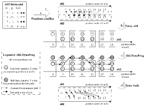
Figure 1: An idealized example of the fuzzy-add strategy. (a) Suppose the current AFPs to add are in AFP list, if we directly add them to one-to-one correspondence set, there will occur position conflict. (b) If we extend ali2 to ali3 with the second dimension limit (ali3_TOT) set to 2, then we may directly add AFPs without considering their position conflict. (c) We may use dynamic programming to find an optimal path which maximizes a given score. (d) The optimal path can be traced back, which is just our one-to-one correspondence set.

• Ali3-DynaProg
  

The purpose of alignment is to get an one-to-one correspondence set between two proteins, and a natural method that converts one-to-multi to one-to-one is dynamic programming DynaProg (see Fig. 1(c)). In details, we design three temporary data structures, called sco3, pos3 and pre3, to record the best score through the dynamic programming path, the best position associated with ’Null-State’ (see below) and the traceback pointer, respectively. Their first dimension is just the same as ali3, however the second dimension is one more than ali3, the extra state is called ’Null-State’ which deals with gaps (shown in Fig. 1(legend)).

• Ali3-DynaProg:

  Recursion: for(i=0; i$<$moln2-1; i++)
  -------------------------------------------------
  01] for(x=0; x$\leq$N[i+1]; x++){
  02]     if(x==0){ // Null-State
  03]         sco3[i+1][x] = MAX(k=0; k$\leq$N[i]; k++){
  04]             sco3[i][k] };
  05]         pos3[i+1][x] = pos3[i][k_max];
  06]         pre3[i+1][x] = k_max; }
  07]     else{     // Real-State
  08]         sco3[i+1][x] = MAX(k=0; k$\leq$N[i]; k++){
  09]             sco3[i][k]+
  10]             GAP_FUNCTION(i+1, x; i, k)+
  11]             SCORE_FUNCTION(i+1, x) };
  12]         pos3[i+1][x] = ali3[i+1][x];
  13]         pre3[i+1][x] = k_max; }}
  

N[k] is the total corresponding points of ali3[k], less than ali3_TOT. k_max is the k that maximizes the MAX function. This is the main dynamic programming function, where,

• 01] GAP_FUNCTION(i+1, x; i, k){
  02]     cur_pos=ali3[i+1][x];  // current position at mol1
  03]     bak_pos=pos3[i][k];    // last position at mol1
  04]     if(cur_pos$>$bak_pos+1){      // sequential gap
  05]         return FOR_GAP+(cur_pos-bak_pos)*EXTEND; }
  06]     else if(cur_pos==bak_pos+1){ // no gap
  07]         return 0; }
  08]     else{                       // non-sequential gap
  09]         return BAK_GAP; }}
  

  01] SCORE_FUNCTION(i+1, x){
  02]     ii=ali3[i+1][x];     // position at mol1
  03]     jj=i+1;                // position at mol2
  04]     score =
  05]         weight1*TM-score(ii,jj) +
  06]         weight2*Vect-score(ii,jj);
  07]     return SCALE*score;}
  

There is an important result needed to point out, though dynamic programming is applied, we may still get non-sequential alignment. This is because the path of Ali3-DynaProg is sequential to mol2, regardless of the corresponding position in mol1. However, we know that such situation will not often happen, so we set non-sequential gap penalty a relatively more negative value than sequential one, in order to punish the former.

• $$\begin{split}TM\mbox{-}score(ii,jj)\end{split}$$ (8)

  01] p1 = mol1[ii];
  02] p2^′ = mol2[jj];
  03] p2 = ROTMAT*p2^′;
  04] tm_score = 1.0/(1.0+($|$p1-p2$|$/d₀)²);
  

  $$\begin{split}Vect\mbox{-}score(ii,jj)\end{split}$$ (9)

  01] v1 = mol1[ii]-mol1[ii-1];
  02] v2^′ = mol2[jj]-mol2[jj-1];
  03] v2 = ROTMAT*v2^′;
  04] vect_score = 1.0*dot(v1,v2)/ ($|$v1$|$ * $|$v2$|$);
  

the range of TM-score(ii,jj) is from 0.0 to 1.0, while Vect-score(ii,jj) is from -1.0 to 1.0. We arbitrarily set the Ali3-DynaProg’s parameters as follows: SCALE = 100, BAK_GAP = 200, FOR_GAP = 50, EXTEND = 5, and it works well.

After we’ve applied the Ali3-DynaProg, the optimal path that maximize the score can be traced back, which is automatically transferred to an one-to-one correspondence set, that is ali1 and ali2 (shown in Fig. 1(d)). The computation time of Ali3-DynaProg grows as O(ali3_TOT*moln2).

II.2.3 Vect-Elong strategy

• Vect-score

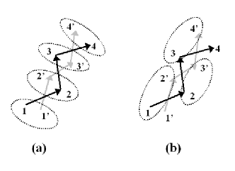
Figure 2: An idealized example of fragment dislocation misalignment situation, point (1,2,3,4) in dark belongs to mol1, point (1’,2’,3’,4’) in gray belongs to mol2. (a) The fragment dislocation misalignment, with point-pairs $<$1,1’$>$, $<$2,2’$>$, $<$3,3’$>$ and $<$4,4’$>$. (b) The reasonable alignment, with point-pairs $<$1,2’$>$, $<$2,3’$>$ and $<$3,4’$>$.

If we measure two protein structures’ alignment only rooted in its point-pair’s Euclidean distance, then the situation called fragment dislocation misalignment (see Fig. 2) is likely to happen, where the fragment aligned by a certain algorithm does not stay at its best location, especially in beta-sheet, with one to four residues deviation.

For example, even the alignment’s RMSD may be relatively low in Fig. 2(a), it’s not as reasonable as the alignment illustrated in Fig. 2(b), where the C_β residues are in the same orientation. Such measuring method based on Euclidean distance may be called ’Dist-score’ (e.g., cRMS, TM-score, etc).

An effective solution to the above problem is to introduce an extra measuring method, called ’Vect-score’ (see Eq. (9)). Based on Vect-score, the alignment in Fig. 2(b) will certainly get a higher score than the alignment in Fig. 2(a). ProSup also finds a similar example and applies a different strategy called ’C_β filter’ to eliminate such cases.

• Vect-Elong

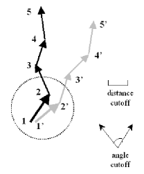
Figure 3: An idealized example of Vect-Elong strategy, point (1,2,3,4,5) in dark belongs to mol1, point (1’,2’,3’,4’,5’) in gray belongs to mol2. After we have identified two proteins’ alignment core which all point-pairs in the core are within the distance cutoff as in the figure (we use the dotted circle to indicate them), we’ll of course miss the SFP(3,3’;3) that satisfies the local flexible condition. If we then apply Vect-Elong with the angle cutoff in the figure as our parameter, the SFP(3,3’;3) will be added to the correspondence set.

Another important usage of Vect-score is to deal with the local flexible situation (Fig. 3) defined as follows, when we have identified two proteins’ alignment core which all point-pairs in the core are within the distance cutoff, there may exist an AFP (Full_AFP or Part_AFP) outside the core which meets the following two features: (a) one terminal of the AFP, whose distance is within the distance cutoff, while the other terminal is beyond the cutoff; (b) the AFP’s corresponding point-pairs are on basically the same direction.

Vect-Elong is such a procedure to solve local flexible that based on Vect-score. We starting from the refined correspondence set, checking one of these corresponding point-pairs (for example, $<$ii,jj$>$) whether or not can be extended to blank portion (i.e., none of the position in point-pair $<$ii+1,jj+1$>$ has corresponding ones). If the point-pair to be tested is blank, and its Vect-score is within a given threshold, we will add this point-pair to the correspondence set, and the extension continues.

Fig. 3 for example, if we use an extension procedure simply based on Dist-score, then for a given distance cutoff, $<$3,3’$>$, $<$4,4’$>$, $<$5,5’$>$, these three point-pairs with obvious local similarity will not be added. While we apply Vect-Elong (using angle cutoff), all these three point-pairs now can be added.

II.3 The flowchart and details of CLeFAPS

An overview of CLeFAPS is presented in Fig. 4 (see Supplementary Table II for default parameters). Though the framework is similar as CLePAPS CLePAPS , the details of every step is totally different (see Supplementary for algorithmic comparison).

II.3.1 SFP generating

We use seed-explosion strategy to generate two lists of SFPs. The seed-explosion strategy is similar as BLAST blast , where we first seek short SFPs at a given length (LEN_L) and a minimal threshold (THRES_L) (we may call these short SFPs seed), then we extend the seed at both terminals. The similar strategy is also used by MUSTANG and MATT to create their SFPs, while the difference is that MUSTANG uses cRMS as their similarity metric and the extension (only at the C-termini) won’t stop until the similarity metric is below the given threshold MUSTANG , MATT also uses cRMS but their SFP’s length is from 5 to 9 MATT .

We set an extension limit (LEN_H) and a threshold (THRES_L) for SFP_L. Then we check the extended SFP’s average score is more than THRES_H or not, if it passes the check, we start a second extension phase whose extension limit is 2*LEN_H and the threshold is THRES_H to create SFP_H. The extension phase stops either the current SFP’s average score is below the given threshold, or it’s length is beyond the extension limit. After generating these two lists, we sort them by CLESUM score, respectively. This step grows O(w1*n²), where n is the longer protein length, and w1=LEN_H+LEN_L. In real program we use redundancy shaving procedure that we only keep the SFP with the highest score among the nearby SFPs CLePAPS . (For details of the pseudo code, see Supplementary, the same as follows.)

We recommend to set the parameters above as follows, LEN_L=6, LEN_H=9. So the SFP_L is from 6 to 8, and the SFP_H is from 9 to 18. Length 6-8 is necessary for including most SFPs with local similarity, while length 9-18 will exclude as many SFPs that only have local coincidence as possible, especially in helix regions whose average length is about ten CLePAPS .

II.3.2 Select the best pivot_SFP

We select the best pivot_SFP from TopK of SFP_H according to its TM-score calculated by fuzzy-adding all AFPs from SFP_H. At the same time, we get the initial ROTMAT according to kabsch2 . This step grows O(TopK* SFP_H’s size), where the average space complexity of SFP_H’s size is about one third of SFP_L’s and its size is approximately O(1/LEN_H* n²). (See time complexity analysis in Supplementary.)

We recommend the parameter TopK be 10, that is to say, we’ll do at most 10 recursions to select the best pivot_SFP. This heuristics is greedy, but it is based on the fact that, if two proteins have global similarity, the chance that we cannot find one SFP in the final alignment from the top ten of SFP_H is relatively small. Actually, our result shows that, at the large database SABmark, the failure alignment because of this situation (none of top 10 is in the final alignment) is rare.

II.3.3 Zoom-in strategy

We apply ZOOM_ITER=3 zoom-in iterations to add AFPs from SFP_L. First, we use the initial ROTMAT from the upper step; then at k-th iteration we check TopNum of SFP_L for AFPs, where,

$$TopNum=\left\{{\begin{array}[]{*{20}c}{\sum\limits_{i=1}^{k}{2^{-i}}}&{k<ZOOM\_ITER}\\ 1&{k=ZOOM\_ITER}\\ \end{array}}\right.$$ (10)

meanwhile we gradually lower our distance cutoff by MINUS, where,

$$MINUS=\frac{INI\_{}CUT-FIN\_{}CUT}{ZOOM\_{}ITER}$$ (11)

For instance, at the first iteration, we check top 1/2 (half) of SFP_L and the distance cutoff is INI_CUT-MINUS, while at the final iteration, we check all of SFP_L and the cutoff is FIN_CUT. At each iteration, we also use fuzzy-add to add AFPs, then use Ali3-DynaProg to get COR which updates ROTMAT. Moreover, we modify the marking procedure in CLePAPS slightly, if one SFP in SFP_L has none point-pairs within the distance cutoff, we mark it ’-1’, then in the later iteration we’ll skip the SFP marked ’-1’. This step grows O(ZOOM_ITER*SFP_L’s size) as the worst complexity, however, the introducing of marking procedure reduces it to O(SFP_L’s size).

II.3.4 Refinement

We apply an recursion of maximal REFINE_ITER=10 iterations to refine our correspondence set under the final distance cutoff (FIN_CUT), each iteration is constituted by the following three procedures:

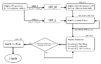
Figure 4: An overview of the CLeFAPS algorithm. Words in italic are the parameters used in related steps.

• Dist-Elong: similar as Vect-Elong (see §II.2.3), with the different that the elongation metric is based on point-pair’s distance instead of Vect-score, and the threshold is FIN_CUT instead of ANG_CUT.

• Partial-add: if one AFP(ii,jj;len) satisfies the distance cutoff, its neighbor AFP(ii,jj+k;len), (where -1*RANGE$\leq$k$\leq$RANGE) may also satisfy the cutoff (we call such case partial-move, there is an excellent illustration in CE’s testcase (1col:A with 1cpc:L) CE that before and after optimization are obviously different). So when the COR has been identified, we may apply partial-add to find each AFP’s adjacent neighbors, then fuzzy-add all these AFPs to ali3. We set RANGE=4 as default for the reason that: first, the period of helix is about four C_α residues so it may help to deal with fragment dislocation at helix region; second, for the other situations except helix, the maximal distance between four C_α’s length is about 15.0Å, which is near our maximal distance cutoff, beyond which may we basically say that the point-pair do not have obvious structural correspondence.

• Ali3-DynaProg: different from the above steps (§II.3.2 and §II.3.3) which only use TM-score as its SCORE_FUNCTION, this step uses both TM-score and Vect-score for the purpose to eliminate fragment dislocation, and setting equal weight works well.

At the end of each refinement iteration, we’ll apply the following criteria to check whether to break or not.

• Break criteria:

  01] if(Failure_Count $\geq$ FAILURE_CUT){ //failure count judge
  02]     break; }
  03] if(TM_Cur $>$ TM_Max ){            //TM-score judge
  04]     Failure_Count=0;
  05]     TM_Max = TM_Cur;
  06]     ROTMAX = ROTCUR; }
  07] else if(TM_Cur $<$ 0.95* TM_Max)break;
  08] else Failure_Count++;
  

where Failure_Count is the counts of failure that the current TM-score (TM_Cur) is less than the maximal TM-score (TM_Max), the default value for FAILURE_CUT is 2, that is to say, if two continuous recursions cannot make the TM-score better than the maximal one, we’ll break the refinement recursion (this made the average recursion to about 3-4).

The purpose of the refinement step in our algorithm is similar as in CE et al. (CE ; ProSup ; FATCAT ; TMalign ; FengSippl ). While the main difference of ours and theirs is that, CLeFAPS can be run in O(n) time, however CE et al. use dynamic programming on the distance matrix calculated using every point-pairs from mol1 and mol2 under current ROTMAT so their time complexity is O(n²).

II.3.5 Vect-Elong

After refinement, we got the optimized COR where every point-pair is within the final distance cutoff. However, since we know that there may exist local flexible situation, it is recommended to apply Vect-Elong at the final stage with the parameter ANG_CUT to be 0.6, which will lead to good result.

III Result

III.1 Examples of applying Vect-score and Vect-Elong

Here, we’ll show the following two cases, with comparison of the four typical algorithms (i.e., CLeFAPS, CLePAPS, CE and MATT, the same as follows) to show the usage of Vect-score and Vect-Elong.

Figure 5: Visualization of superposition of dark structure (PDB_ID 1bxd,chain:A,290-450) and gray structure (PDB_ID 1b3q,chain:A,355-540) in HOMSTRAD family Histidine_Kinase. Details of the fragment dislocation misalignment from (b) CLePAPS and (c) CE; The reasonable alignment from (a) CLeFAPS and (d) MATT.
Note: residues not placed into the alignment by the algorithms are shown in thin lines while those in the alignment are shown in bold lines. The pictures were generated by RasMol RasMol .

III.1.1 Employment of Vect-score to solve fragment dislocation

1bxd(chain:A,290-450) and 1b3q(chain:A,355-540) are two protein domains in the Histidine_Kinase family of HOMSTRAD. The fragment dislocation misalignment (in beta-sheet) of CE and CLePAPS are shown in Fig. 5(c) and Fig. 5(b), respectively. CLeFAPS employs TM-score plus Vect-score as the SCORE_FUNCTION of Ali3-DynaProg in the refinement step to eliminate such situation (shown in Fig. 5(a)). The result is supported by MATT (shown in Fig. 5(d)).

III.1.2 Employment of Vect-Elong to solve local flexible

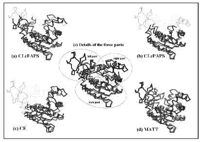
Figure 6: Visualization of superposition of dark structure (PDB_ID 1ake) and gray structure (PDB_ID 4ake) aligned by the following algorithms: (a) CLeFAPS, (b) CLePAPS, (c) CE and (d) MATT. (e) Details of the three parts: core part, left part and right part. Cyan structure in left part and right part is the original position of 4ake, while blue structure in left part and right part is the individual superposition of 1ake and 4ake based on the correspondences in left part and right part, respectively.

The adenylate kinase protein (AKE) has a stable inactive conformation, in addition to an active form, i.e., the open and closed forms FlexProt . They are represented by PDB_ID 4ake and 1ake, respectively. The protein can be cut into three parts according to ake , which may be called the rigid part (core part), the LID domain (right part) and the NMP_bind domain (left part), respectively (shown in Fig. 6(e)). The result alignment of the four algorithms are shown in Fig. 6(a) to 6(d). CLePAPS found the core part, CE found both the core and the right part, while in right part, CE didn’t give an accurate alignment. CLeFAPS first found the core part similar as CLePAPS, then it applied Vect-Elong to find the left and the right part, though incompletely, for the reason that CLeFAPS is based on the rigid-body framework. MATT did the best job to find all three parts completely, however it cost the most runtime.

III.2 Different types of proteins for alignment

We consider the following four different types of proteins, small size, large size, closely-related and distantly-related. We’ll talk the former two types in this subsection while the latter two types will be discussed in the following subsection §III.3 and §III.4.

III.2.1 Small proteins

Figure 7: Visualization of superposition of d1r5pa_ (dark) and d1t4za_ (gray) in SCOP superfamily (c.47.1) aligned by CLeFAPS with different lower boundary. (a) Lower boundary=3.0, with the result of TM-score=0.362, LALI=45 and RMSD=2.692. (b) Lower boundary=4.0 with the result of TM-score=0.376, LALI=48 and RMSD=2.742. (c) Lower boundary=5.0 (default) with the result of TM-score=0.442, LALI=63 and RMSD=3.280.

d1r5pa_ (90 residues) and d1t4za_ (105 residues) belong to the SCOP Thioredoxin-like superfamily (c.47.1) (we use the structures in the ASTRAL(40%) compendium ASTRAL ). We’ve tried different lower boundary for the association of d₀ with the distance cutoff, from 3.0, 4.0 to 5.0Å (shown in Fig. 7). The d₀ factor in this case is 3.4059Å (see Eq. (3)), and the amino acid identity of this pair is 27.0%. If we set the lower boundary too small (e.g., 3.0 or 4.0Å), the final distance cutoff (FIN_CUT) will directly be associated with d₀ (see Eq. (II.2.1)), and then we’ll miss some obviously alignable regions when dealing with such small but distantly related proteins. However, if we set the lower boundary at a moderate value (i.e., 5.0Å), then when dealing with proteins whose length is below 180 residues, the final distance cutoff is constant at 5.0Å (see Eq. (3,II.2.1)), and such value is tolerant for adding AFPs in small (or moderate) size but distantly related proteins.

III.2.2 Large proteins

d1twfb_ (1094 residues) and d2a69c1 (1119 residues) belong to the SCOP beta and beta-prime subunits of DNA dependent RNA- polymerase superfamily (e.29.1). We’ve tried self-adaptive strategy (association of d₀ with the average CLESUM score’s threshold) and constant values. The d₀ factor in this case is 10.91Å, using Eq. (II.2.1,7) we get the self-adaptive threshold (THRES_L=5 and THRES_H=20), then the SFP lists’ size is 5635 of SFP_H and 63644 of SFP_L, respectively. Using constant values (THRES_L=0 and THRES_H=15) however, the two SFP lists’ size is 10962 of SFP_H and 83737 of SFP_L. As a result we get the similar alignment with correspondence identity at 94.3%, while the running time of self-adaptive strategy is 30% faster than that of constant values. Moreover, from the comparison of the four algorithms, CLeFAPS gets the best TM-score 0.720 and the largest alignment length 851 while the other three get the similar TM-score (about 0.61) and the similar alignment length (about 700). This is not surprising, because CLeFAPS employs the final distance cutoff (FIN_CUT) at 10.91Å so it will collect more alignable regions than the other algorithms which set their parameters constant for general purposes instead of such large proteins.

III.3 CLeFAPS’s performance on HOMSTRAD families

HOMSTRAD is a database of protein structural alignments for homologous families HOMSTRAD . Its alignments were generated using structural alignment programs, then followed by a manual scrutiny of individual cases. There are totally 1033 families (633 at pairwise level). We’ll compare the four algorithms on these 633 families, and the alignment accuracy metric is:

• Correct(algorithm)/LOA(length of algorithm)

  Calculated by comparing every pairwise alignment in a certain algorithm against the reference (HOMSTRAD). All correctly aligned residue pairs in comparison with the reference are considered as Correct and the total alignment length of the certain algorithm as LOA. This is the same metric as ACC used in MUSTANG MUSTANG .

• Correct(algorithm)/LOR(length of reference)

  All correctly aligned residue pairs in comparison with the reference are considered as Correct and the length of alignment in reference is called LOR.

The reason why we develop the second C/LOR metric is as follows, for instance, 1kxr (chain:A,221-352) and 1kfu (chain:L,211-355) are two protein domains in the Peptidase_C2_D2 family of HOMSTRAD and reference length is 130. MATT got an alignment of 93 point-pairs with 93 correct, its C/LOA is 1.0 while its C/LOR is only 0.715. CLeFAPS, however, got an alignment of 123 point-pairs with 116 correct, its C/LOA is 0.943 while its C/LOR is 0.892.

Table 1: Alignment accuracy metric on HOMSTRAD from CLeFAPS, CLePAPS, CE and MATT

Accuracy metric	CLeFAPS	CLePAPS	CE	MATT
C/LOA1	0.929	0.916	0.911	0.948
C/LOR2	0.898	0.847	0.881	0.831
1: Correct/Length of the algorithm.
2: Correct/Length of the reference.

From the data in Table 1, MATT scored highest in C/LOA but lowest in C/LOR. On the contrary, CLeFAPS scored highest in C/LOR and second highest in C/LOA. This is because MATT allows local flexibilities (or bent) everywhere between short fragments (i.e., AFPs) and then uses dynamic programming to assembly these bentable AFPs. However, MATT didn’t apply the final optimization procedure, which is used in CE and CLeFAPS, so the alignment length of MATT is relatively small while the precision is relatively high. CLePAPS, analogously, greedy-add all AFPs and then skip the final optimization procedure, get a relatively high C/LOA and low C/LOR as MATT.

III.4 CLeFAPS’s performance on the discrimination problem

The discrimination problem, takes as input a pair of protein structures, and is supposed to output a yes/no answer (together with an assessment score) as to whether a good alignment can be found for these two protein structures or not MATT . In our article, we followed MATT’s method and take SABmark SABmark ’s superfamily as our test set, which is natural for the discrimination problem because: (a) it contains 3645 domains sorted into 425 subsets representing structures at SCOP superfamily level, each SABmark subset contains at most 25 structures, which can be regarded as plus set; (b) it additionally provides a set of decoy structures for nearly all its 425 sets, each decoy’s sequence is similar to its corresponding set while its structure is within a different SCOP fold, each decoy set contains at most 25 structures, which can be regarded as minus set.

We constructed the following two decoy discrimination test, one is similar as MATT that for each superfamily we choose a random pair of structures both from plus set (can not be the same) and a random pair from plus and minus set, we call such procedure RANDOM test. The other is that we conduct all-against-all within plus set and between plus and minus set, we call such procedure All-Against-All test.

When comparing the four algorithm’s ROC curves ROC , SABmark now serves as the gold standard. For varying thresholds based on a certain assessment function, all pairs below the threshold are assumed positive, and all above it negative. The pairs that agree with the standard are called true positives (TP) while those that do not are false positives (FP) ROCcurve .

Table 2: Comparison of LALI+RMSD and TM-score based on MATT’s performance on SABmark

True Positive	LALI+RMSD	TM-score
95.04	71.16	86.0
94.09	75.65	87.5
93.14	77.30	88.4
92.20	79.20	90.3
91.02	82.74	91.7
90.07	86.52	93.4
True Negative
Note:
(1) the LALI+RMSD data is from MATT MATT .
(2) the discrimination test is RANDOM test.
(3) True_Negative%+False_Positive%=100.0%

First, we compare the assessment function of TM-score and LALI+RMSD based on the same algorithm (MATT) and the same decoy discrimination test (RANDOM test) (see Table 2) MATT , at each fixed true positive rate, TM-score got a nearly 10% higher true negative rate than LALI+RMSD.

Table 3: AUC values based on TM-score from CLeFAPS, CLePAPS, CE and MATT

Discrimination test	CLeFAPS	CLePAPS	CE	MATT
RANDOM	0.970	0.932	0.966	0.974
All-Against-All	0.952	0.912	0.956	0.964

Second, we compare ROC curves and AUC topsfatcat over the four algorithms (shown in Fig. 8 and Table 3), MATT performs best in both tests and CE follows the second, while CLeFAPS is comparable with CE and is better than CLePAPS. A notable result when comparing CLePAPS and CLeFAPS is, in RANDOM test CLePAPS failed 9/425 in positive test and 49/425 negative test while CLeFAPS only failed 1/425 in the former test; in All-Against-All test CLePAPS failed 1322/40676 in positive test and 4064/40066 negative test while CLeFAPS failed 28/40676 in former and 75/40066 in latter. This result may be the demonstration that, CLeFAPS employing the seed-explosion strategy to create SFP_H is more effective than CLePAPS employing fixed parameters.

Table 4: Runtime of All-Against-All test from CLeFAPS, CLePAPS, CE and MATT

Runtime (sec)	CLeFAPS	CLePAPS	CE	MATT
Total runtime	1259	1136	61669	172812
Average runtime	0.01526	0.01377	0.74765	2.09510
Note: All-Against-All test contains 80742 pairs of proteins.

Finally, we compare running (see Table 4) using the Windows XP operation system with 2*2.66-GHz Dual-Core Intel CORE 2 Dual processor and 2-GB 667 MHz memory. The result is on All-Against-All test which contains 80742 pairs of proteins. We find that, though MATT and CE perform best and second best (comparable with CLeFAPS) on the discrimination problem, they are the slowest and the second slowest on running time, while CLeFAPS and CLePAPS takes only about 1/50 of the running time used by CE and 1/150 of MATT, and CLeFAPS is only 10% more than CLePAPS.

(a) RANDOM discrimination test

(b) All-Against-All discrimination test

Figure 8: The ROC curve analysis based on TM-score obtained from CLeFAPS, CLePAPS, CE and MATT.

IV Discussion and future work

We proposed the program called CLeFAPS, which considers protein’s flexibility based on a rigid-body framework, instead of introducing twists (bends). The result showed that when dealing with the structural distortion caused by distantly related proteins through evolution FATCAT , CLeFAPS is competitive with those algorithms that allow twists, and the reasons are as follows,

• Through the incorporation of d₀ factor from TM-score to associate the main parameters of the pairwise alignment, including the similarity metric of SFP (CLESUM score threshold) and the consistency metric in pile-up of the alignment (distance cutoff), with the size of the input proteins (Parameter self-adaptive).

• Through the enlargement of the one-to-one correspondence set to one-to-multi during the pile-up procedure, which collects all AFPs while neglecting their position conflict (Fuzzy-add). Then applying dynamic programming, which uses TM-score (or plus Vect-score) as the objective function, to get an optimal alignment path (Ali3-DynaProg).

• Through the elongation based on the Vect-score to collect local flexible fragments, that the fragment’s point-pairs are exceed the final distance cutoff while they share local structural similarity, after we’ve identified two proteins’ alignment core (Vect-Elong).

Furthermore, we employ TM-score as the assessment function to measure the structural similarity between two proteins, which has been demonstrated effective by comparing the result on the discrimination test.

Perhaps the most highlighted feature of CLeFAPS is its fast speed, where the most important contribution is the TopK(=10) cutoff in the step called select the best pivot_SFP (see §II.3.2), where we’ll do at most TopK(=10) recursions. If all these TopK(=10) SFPs in SFP_H are far away from the final alignment, the algorithm will certainly end in failure. In the future work, we’ll start a precise exploration on the accuracy of TopK SFPs in SFP_H through the statistics on some large databases.

There is another structural distortion caused by conformational flexibility FATCAT , say, domain motion domainmove . However, CLeFAPS is ineffective to deal with such cases because of its rigid-body framework while it can only deal with local flexible fragments. When an entire domain undergoes a significant conformational change, we may use the Multi-solution strategy CLePAPS ; ProSup to solve it.

CLeFAPS is a sequence-independent structural alignment algorithm, however if we consider the amino acid, the generalized conformational letter (reduction of amino acid plus conformational letter) cle2 may be employed to encode the input proteins and the generalized CLESUM cle2 be applied to generate the SFP list. It is expected that through this procedure may we get more accurate result as well as reduce the TopK’s failure rate.

Supplementary Data

Supplementary Data are available at ….

References

- (1) Koehl,P., 2006, Protein Structure Classification, Chapter 1 of Reviews in Computational Chemistry,V. 22, ed. KB. Lipkowitz, TR. Cundari, and VJ. Gillet, Wiley-VCH, John Wiley and Sons, Inc., 2006.
- (2) I Eidhammer, I Jonassen, WR Taylor, Structure comparison and structure patterns, J. Comput. Biol. 2000; 7:685-716.
- (3) Irving JA, Whisstock JC, Lesk AM (2001) Protein structural alignments and functional genomics. Proteins 42: 378-382.
- (4) Edgar R, Batzoglou S (2006) Multiple sequence alignment. Curr Opin Struct Bio 16: 368-373.
- (5) Dunbrack RL (2006) Sequence comparison and protein structure prediction. Curr Opin Struct Biol 16: 274-284.
- (6) Chandonia,J.-M., Hon,G., Walker,N.S., Conte,L.L., Koehl,P., Levitt,M. and Brenner,S.E. (2004) The ASTRAL Compendium in 2004. Nucleic Acids Res., 32 (Database issue), D189-D192.
- (7) Murzin,A.G., Brenner,S.E., Hubbard,T. and Chothia,C. (1995) SCOP:a structural classification of proteins database for the investigation of sequences and structures. J. Mol. Biol., 247, 536-540.
- (8) Orengo,C.A., Michie,A.D., Jones,S., Jones,D.T., Swindells,M.B. and Thornton,J.M. (1997) CATH-a hierarchic classification of protein domain structures. Structure, 5, 1093-1108.
- (9) Holm, L. and Sander, C. (1996). The FSSP database: Fold classification based on structure-structure alignment of proteins. NAR, 24 (1), 206-209.
- (10) Yang,J.M. and Tung,C.H. (2006) Protein structure database search and evolutionary classification. Nucleic Acids Res., 34, 3646-3659.
- (11) Berman,H.M., Westbrook,J., Feng,Z., Gilliland,G., Bhat,T.N., Weissig,H., Shindyalov,I.N. and Bourne,P.E. (2000) The Protein Data Bank. Nucleic Acids Res., 28, 235-242.
- (12) Goldman D, Istrail S, Papadimitriou CH (1999) Algorithmic aspects of protein structure similarity. In: Beame P, editor. Proceedings of the 40th Annual Symposium on Foundations of Computer Science. Los Alamitos (California): IEEE Computer Society. pp. 512-522.
- (13) Holm,L. and Sander,C. (1993) Protein structure comparison by alignment of distance matrices. J. Mol. Biol., 233, 123-138.
- (14) Shindyalov,I.N. and Bourne,P.E. (1998) Protein structure alignment by incremental combinatorial extension (CE) of the optimal path. Protein Eng., 11, 739-747.
- (15) Wang,S., Zheng,W.M., CLePAPS: Fast Pair Alignment of Protein Structures based on Conformational Letters. J. Bioinform. Comput. Biol. 2008 Apr;6(2):347-66.
- (16) Lackner,P., Koppensteiner,W.A., Sippl,M.J., and Domingues,F.S. ProSup: a refined tool for protein structure alignment, Protein Engineering, 2000; 13: 745-752.
- (17) Ye Y, Godzik A (2003) Flexible structure alignment by chaining aligned fragment pairs allowing twists. Bioinformatics (Supplement 2): II246-II255.
- (18) Shatsky M, Nussinov R, Wolfson H (2002) Flexible protein alignment and hinge detection. Proteins 48: 242-256.
- (19) Menke M, Berger B, Cowen L (2008) Matt: Local flexibility aids protein multiple structure alignment. PLoS Comput Biol 4(1): e10. doi:10.1371/journal.pcbi.0040010.
- (20) Konagurthu A, Whisstock J, Stuckey P, Lesk A (2006) MUSTANG: A multiple structural alignment algorithm. Proteins 64: 559-574.
- (21) Needleman,S.B., and Wunsch,C.D. A general method aplicable to the search for similarity in the amino acid sequence of two proteins. J. Mol. Biol., 1970; 48: 443-454.
- (22) Zheng,W.M. and Liu,X. A protein structural alphabet and its substitution matrix CLESUM. Lecture notes in Bioinformatics 3680 (eds. C. Priami and A. Zelikovsky), Springer Verlag, Berlin, 2005: 59-67;
- (23) Zheng,W.M. The Use of a Conformational Alphabet for Fast Alignment of Protein Structures.
- (24) Jacobs,D.J., Rader,A.J., Kuhn,L.A. and Thorpe,M.F. (2001) Protein flexibility predictions using graph theory. Proteins, 44, 150-165.
- (25) N. Echols, D. Milburn, M. Gerstein. MolMovDB: analysis and visualization of conformational change and structural flexibility. Nucleic Acids Research, 31:478-482, 2003.
- (26) M. Veeramalai, Y. Ye and A. Godzik. (2008) TOPS++FATCAT: fast flexible structural alignment using constraints derived from TOPS+ Strings Model. BMC Bioinformatics ,9:358, 2008.
- (27) Kabsch W. A discussion of the solution for the best rotation to relate two sets of vectors. Acta Cryst 1978;A 34:827-828.
- (28) Zhang Y, Skolnick J. TM-align: a protein structure alignment algorithm based on TM-score. Nucl Acid Res 2005;77(7):2302-2309.
- (29) Zhang,Y. and Skolnick,J. (2004) Scoring function for automated assessment of protein structure template quality. Proteins, 57, 702-710.
- (30) Kolodny R, Koehl P, Levitt M (2005) Comprehensive evaluation of protein structure alignment methods: Scoring by geometric measures. J Mol Biol 346: 1173-1188.
- (31) Gribskov,M. and Robinson, N. L. (1996). Use of receiver operating characteristic (ROC) analysis to evaluate sequence matching. Comput. Chem. 20, 25-33.
- (32) Kleywegt, G. J. and Jones, A. (1994). Superposition. CCP4/ESF-EACBM Newsletter Protein Crystallog. 31,9-14.
- (33) Levitt M, Gerstein M (1998) A unified statistical framework for sequence comparison and structure comparison. Proc Natl Acad Sci U S A 95: 5913-5920.
- (34) Siew N, Elofsson A, Rychlewski L, Fischer D. MaxSub: an automated measure for the assessment of protein structure prediction quality. Bioinformatics 2000;16(9):776-785.
- (35) Altschul, S. F., Madden, T. L., Schaffer, A. A., Zhang, J. H., Zhang, Z., Miller, W. and Lipman, D. J. (1997). Gapped BLAST and PSI-BLAST: a new generation of protein database search programs. Nucl. Acids Res. 25, 3389-3402.
- (36) Mizuguchi K, Deane C, Blundell TL, Overington J (1998) HOMSTRAD: A database of protein structure alignments for homologous families. Protein Sci 11: 2469-2471.
- (37) VanWalle I, Lasters I, Wyns L (2005) SABmark-A benchmark for sequence alignment that covers the entire known fold space. Bioinformatics 21: 1267-1268.
- (38) Feng,Z.K. and Sippl,M.J. (1996) Optimum superimposition of protein structures: ambiguities and implications. Fold Des., 1, 123-132.
- (39) Günther, J., Bergner, A., Hendlich, M. and Klebe, G. Utilising structural knowledge in drug design strategies-applications using Relibase. J. Mol. Biol. 326: 621-636.
- (40) Sayle, R. A. and Milner-White, E. J. (1995) RASMOL: biomolecular graphics for all. Trends Biochem. Sci. 20, 374.