Introduction to Millimeter/Sub-Millimeter Astronomy

1 Introduction

This chapter provides an introduction to the following lectures. It is based on nine lectures given at the Saas Fee school in March 2008. Much, but not all of this material is contained in RW4 and RW5 , but with more more emphasis on current research in millimeter/sub-millimeter astronomy. In the following, the basics of radiative transfer, receivers, antennas, interferometry radiation mechanisms and molecules are presented. The field of mm/sub-mm astronomy has become very large, so this presentation contains only a few derivations. The astute reader will note that Maxwell’s Equations do not appear at all, although the results are based on these. In some cases, the approach is to quote a result followed by an example. This contribution is aimed at graduate students with a good background in physics and astronomy. Some common terms are used but ^′′jargon^′′ has been avoided as much as possible. References are given, for the most part, to more recent work where citations to earlier work can be found. The units are mostly CGS with some SI units. This follows the usage in the astronomy literature. One topic not covered here is polarization; see RW4 and THUM for an introduction.

The field of mm/sub-mm astronomy began only in the 1960’s, but the richness of the results has justified this series of lectures. Millimeter/sub-mm measurements require excellent weather, very accurate antennas, and sensitive receivers. The interpretation of these data requires a knowledge of atomic and molecular physics, radiative transfer and interstellar chemistry. By number, about 90% of molecular clouds consist of H₂. However, the determination of local densities and column densities of molecular hydrogen, H₂ must be indirect since H₂ does not emit spectral lines in cooler clouds. The Schrödinger equation governs all chemistry, but the conditions in the interstellar medium are very different (and much more varied) than those on earth. Earth-bound chemistry is only a subset of the more general interstellar chemistry; it is dominated by non-equilibrium processes that occur at low temperatures and densities, so determinations of collision and reaction rates are needed. A project devoted to this goal is the ^′′Molecular Universe^′′ (see the web site for details). For an overview of interstellar chemistry, the reader is referred to the short presentation HERBST or the monograph TIELENS . Although interstellar chemistry plays a very important role in molecular line astronomy, it is not included due to space limitations. Another glaring omission is a treatment of the Cosmic Microwave Background (CMB), since this is not treated in the following two lectures. Technically, the CMB emission is not weak, but does fill the entire sky, so special techniques must be employed.

Mm/sub-mm astronomy is one of the most important tools to study the birth of stars STARFORM , PPV and star formation in galaxies LINDA . Stars form in molecular clouds where extinction is large. Thus, near infrared and optical studies are of limited value. At high red shifts, many active star forming galaxies and Active Galactic Nuclei (AGN’s) are enshrouded by dust PHILSOL . Synchrotron emission at cm wavelengths from AGN’s allows sub-arcsecond resolution images of relativistic electrons moving in $\vec{B}$ fields SCHEUER . However, the imaging of dust and molecules on comparable scales is just beginning, so this is an area where important contributions can be made.

The closest example of a supermassive Black Hole is Sgr A^∗, 8.5 kpc (1 kpc=3.08   $\times\,10^{21}$ cm) from the Sun. Sgr A^∗ is quiescent at present, but is thought to be similar to the ^′′engines^′′ that power AGN’s. The radio emission from Sgr A^∗ is interpreted as optically thick synchrotron emission, so with mm/sub-mm Very long Baseline interferometry, gas on Astronomical Unit (1 AU=1.5   $\times\,10^{13}$ cm) scales, close to the Schwarzschild radius, can be sampled.

In the field of star formation, we believe that all of the physical principles are known. However, star formation is complex and measurements are needed to determine which processes are dominant and which can be neglected. In contrast, for studies of the early universe, Black Holes and AGN’s not all of the relevant physical laws may be known. As in all of astronomy, measurements often lead to unexpected results that may have far reaching effects on our understanding of fundamental physical laws.

The dominant continuum radiation mechanism in the mm/sub-mm wavelength range is dust emission. This differs from free-free and synchrotron emission, which is commonly encountered at centimeter wavelengths ENDRIK . Spectral line radiation is dominated by thermal and quasi-thermal molecular radiation, although there are a few important atomic lines of carbon, oxygen and nitrogen.

The sensitivity at mm/sub-mm wavelengths has become about 100 times better than was the case in the 1960’s GURV . However sensitivity alone is not enough to transform the field. Rather, high resolution images are needed. This will change when the Atacama Large Millimeter Array (ALMA) begins operation. ALMA will initially operate between 3.5 mm and 0.4 mm. ALMA has a unique combination of high angular resolution and high sensitivity. This will allow ALMA to transform the field of mm/sub-mm astronomy. A summary of the science planned for ALMA is to be found in ALMA-SCI .

2 Some Background

In this section, we review the basics needed in following sections (see RW4 ). Electromagnetic radiation in the radio window can be interpreted as a wave phenomenon, i. e. in term of classical physics. When the scale of the system involved is much larger than a wavelength, we can consider the radiation to travel in straight lines or rays. The power, ${\rm d}P$, intercepted by a infinitesimal surface ${\rm d}\sigma$ is

$${\rm d}P=I_{\nu}\cos\theta\,{\rm d}\Omega\,{\rm d}\sigma\,{\rm d}\nu$$ (1)

where
${\rm d}P$ = power, in watts, ${\rm d}\sigma$ = area of surface, m², ${\rm d}\nu$ = bandwidth, in Hz, $\theta$ = angle between the normal to ${\rm d}\sigma$ and the direction to ${\rm d}\Omega$, ${\rm I_{\nu}}$ = brightness or specific intensity, in W m^-2 Hz^-1 sr^-1.

Equation (1) is the definition of the brightness $I_{\rm\nu}$. Quite often the term intensity or specific intensity $I_{\rm\nu}$ is used instead of the term brightness. We will use all three designations interchangeably.

The total flux of a source is obtained by integrating (1) over the total solid angle $\Omega_{\rm s}$ subtended by the source

$$S_{\nu}=\int\limits_{\Omega_{\rm s}}I_{\nu}(\theta,\varphi)\cos\theta\,{\rm d}\Omega,$$ (2)

and this flux density is measured in units of W m^-2 Hz^-1. Since the flux density of astronomical sources is usually very small, a special unit, the Jansky (hereafter Jy) has been introduced

$$1\,{\rm Jy}=10^{-26}\,{\rm W\,m}^{-2}{\rm Hz}^{-1}=10^{-23}\,{\rm erg\,s^{-1}}{\rm cm}^{-2}{\rm Hz}^{-1}\thinspace.$$ (3)

As long as the surface element ${\rm d}\sigma$ covers the ray bundle completely, the power remains constant:

$${\rm d}P_{1}={\rm d}P_{2}\thinspace.$$ (4)

From this, we can easily obtain

$$I_{\rm\nu_{1}}=I_{\rm\nu_{2}}$$ (5)

so that the brightness is independent of the distance. The total flux $S_{\rm\nu}$ density shows the expected dependence of $1/r^{2}$.

Another useful quantity related to the brightness is the radiation energy density $u_{\rm\nu}$ in units of erg cm^-3. From dimensional analysis, $u_{\rm\nu}$ is intensity divided by speed. Since radiation propagates with the velocity of light $c$, we have for the spectral energy density per solid angle

$$u_{\rm\nu}(\Omega)=\frac{1}{c}\,I_{\rm\nu}\thinspace.$$ (6)

If integrated over the whole sphere, $4\pi$ steradian, (Eq. 6) will yeild the total spectral energy density

$$u_{\rm\nu}=\int\limits_{(4\pi)}u_{\rm\nu}(\Omega)\,{\rm d}\Omega=\frac{1}{c}\int\limits_{(4\pi)}I_{\rm\nu}\,{\rm d}\Omega\thinspace.$$ (7)

2.1 Radiative Transfer

The equation of transfer is

$$\framebox{$\displaystyle\frac{{\rm d}I_{\nu}}{{\rm d}s}=-\kappa_{\nu}I_{\nu}+\varepsilon_{\nu}$}\quad.$$ (8)

The linear absorption coefficient $\kappa_{\nu}$ and the emissivity $\varepsilon_{\nu}$ are independent of the intensity $I_{\nu}$ leading to the above form for ${\rm d}I_{\nu}$.

In Thermodynamic Equilibrium (TE) there is complete equilibrium of the radiation with its surroundings, the brightness distribution is described by the Planck function, which depends only on the temperature $T$, of the surroundings. The properties of the Planck function will be described in the next section.

In Local Thermodynamic Equilibrium (LTE) Kirchhoff’s law holds

$$\framebox{$\displaystyle\frac{\varepsilon_{\nu}}{\kappa_{\nu}}=B_{\nu}(T)$}$$ (9)

This is independent of the material, as is the case with complete thermodynamic equilibrium. In general however, $I_{\nu}$ will differ from $B_{\nu}(T)$.

If we define the optical depth ${\rm d}\tau_{\nu}$ by

$${\rm d}\tau_{\nu}=-\kappa_{\nu}\,{\rm d}s$$ (10)

or

$$\tau_{\nu}(s)=\int\limits_{s_{0}}^{s}\kappa_{\nu}(s)\,{\rm d}s\thinspace,$$ (11)

then the equation of transfer (8) can be written as

$$\framebox{$\displaystyle-\frac{1}{\kappa_{\nu}}\frac{{\rm d}I_{\nu}}{{\rm d}s}=\frac{{\rm d}I_{\nu}}{{\rm d}\tau_{\nu}}=I_{\nu}-B_{\nu}(T)$}\quad.$$ (12)

The solution of (12) is

$$\framebox{$\displaystyle I_{\nu}(s)=I_{\nu}(0)\,{\rm e}^{-\tau_{\nu}(s)}+\int\limits_{0}^{\tau_{\nu}(s)}B_{\nu}(T(\tau))\,{\rm e}^{-\tau}{\rm d}\tau$}\quad.$$ (13)

If the medium is isothermal,

$$T(\tau)=T(s)=T=\mbox{const.}$$

the integral is

$$\framebox{$\displaystyle I_{\nu}(s)=I_{\nu}(0)\,{\rm e}^{-\tau_{\nu}(s)}+B_{\nu}(T)\,(1-\,{\rm e}^{-\tau_{\nu}(s)})$}\quad.$$ (14)

For a large optical depth, that is for $\tau_{\nu}(0)\rightarrow\infty$, (14) in LTE approaches the limit

$$I_{\nu}=B_{\nu}(T)\thinspace.$$ (15)

This is case for planets and the 2.7 K microwave background. The difference between $I_{\nu}(s)$ and $I_{\nu}(0)$ gives

$$\Delta I_{\nu}(s)=I_{\nu}(s)-I_{\nu}(0)=(B_{\nu}(T)-I_{\nu}(0))(1-{\rm\,e}^{-\tau})\;.$$ (16)

Eq. 16 represents an on-source minus an off-source measurement.

2.2 Black Body Radiation
       and Brightness Temperature

The spectral distribution of the radiation of a black body in thermodynamic equilibrium is given by the Planck law

$$\framebox{$\displaystyle B_{\nu}(T)=\frac{2h\nu^{3}}{c^{2}}\frac{1}{{\rm e}^{h\nu/kT}-1}$}\quad.$$

If $h\nu\ll kT$, one obtains Rayleigh-Jeans Law.

$$\framebox{$\displaystyle B_{\rm RJ}(\nu,T)=\frac{2\nu^{2}}{c^{2}}kT$}\quad.$$ (17)

This is an expression of classical physics in which there is an energy $kT$ per mode. The term $\frac{2\nu^{2}}{c^{2}}$ is the density of states for 3 dimensions. In the millimeter and submillimeter range, one frequently defines a radiation temperature, $J(T)$ as

$$J(T)=\frac{c^{2}}{2k\nu^{2}}\,I=\frac{h\nu}{k}\frac{1}{{\rm\,e}^{{h\nu}/{kT}}-1}\;.$$ (18)

Inserting numerical values for $k$ and $h$, we find that the Rayleigh-Jeans relation holds for frequencies

$$\frac{\nu}{\rm GHz}\ll 20.84\left(\frac{T}{\rm K}\right)\,.$$ (19)

It can thus be used for all thermal radio sources except perhaps for low temperatures in the mm/sub-mm range.

In the Rayleigh-Jeans relation, the brightness and the thermodynamic temperature of the black body that emits this radiation are strictly proportional (17). This feature is so useful that it has become the custom in radio astronomy to measure the brightness of an extended source by its brightness temperature $T_{\rm b}$. This is the temperature which would result in the given brightness if inserted into the Rayleigh-Jeans law

$$T_{\rm b}=\frac{c^{2}}{2k}\frac{1}{\nu^{2}}\,I_{\nu}=\frac{\lambda^{2}}{2k}\,I_{\nu}\thinspace.$$ (20)

Combining (2) with (20), we have

$$\framebox{$\displaystyle S_{\nu}=\frac{2\,k\,\nu^{2}}{c^{2}}T_{\rm b}\,\mbox{\greeksym{D}}\Omega$}\quad.$$ (21)

For a Gaussian source, this relation is

$$\left[\frac{S_{\nu}}{\rm Jy}\right]=0.0736\,T_{\rm b}\,\left[\frac{\theta}{\rm arc\,seconds}\right]^{2}\left[\frac{\lambda}{\rm mm}\right]^{-2}$$ (22)

That is, if the flux density $S_{\nu}$ and the source size are known, then the true brightness temperature, $T_{\rm b}$, of the source can be determined. The concept of temperature in radio astronomy has given rise to confusion. If one measures $S_{\nu}$ and the apparent source size, Eq. 22 allows one to calculate the main beam brightness temperature, T_MB. Details of this procedure will be given in Section 5. The performance of coherent receivers is characterized receiver noise temperature; see Section 3.2.1 for details. The combination of receiver and atmosphere is characterized by system noise temperature; this is discussed in Section 6.1 and following.

If $I_{\nu}$ is emitted by a black body and $h\nu\ll kT$ then (20) gives the thermodynamic temperature of the source, a value that is independent of $\nu$. If other processes are responsible for the emission of the radiation, $T_{\rm b}$ will depend on the frequency; it is, however, still a useful quantity and is commonly used in practical work.

This is the case even if the frequency is so high that condition (19) is not valid. Then (20) can still be applied, but $T_{\rm b}$ is different from the thermodynamic temperature of a black body. However, it is rather simple to obtain the appropriate correction factors.

It is also convenient to introduce the concept of brightness temperature into the radiative transfer equation (16). Formally one can obtain

$$J(T)=\frac{c^{2}}{2k\nu^{2}}(B_{\nu}(T)-I_{\nu}(0))(1-{\rm\,e}^{-\tau_{\nu}(s)})\;.$$

Usually calibration procedures allow one to express $J(T)$ as $T$. This measured quantity is referred to as $T^{*}_{\rm R}$, the radiation temperature, or the brightness temperature, $T_{\rm b}$. In the cm wavelength range, one can apply (20) to (12) and one obtains

$$\framebox{$\displaystyle\frac{{\rm d}T_{\rm b}(s)}{{\rm d}\tau_{\nu}}=T_{\rm b}(s)-T(s)$}\quad,$$ (23)

where $T(s)$ is the thermodynamic temperature of the medium at the position $s$. The general solution is

$$\framebox{$\displaystyle T_{\rm b}(s)=T_{\rm b}(0)\,{\rm e}^{-\tau_{\nu}(s)}+\int\limits_{0}^{\tau_{\nu}(s)}T(s)\,{\rm e}^{-\tau}{\rm d}\tau$}\quad.$$ (24)

If the medium is isothermal, this becomes

$$\framebox{$\displaystyle T_{\rm b}(s)=T_{\rm b}(0)\,{\rm e}^{-\tau_{\nu}(s)}+T\,(1-\,{\rm e}^{-\tau_{\nu}(s)})$}\quad.$$ (25)

2.3 The Nyquist Theorem and the Noise Temperature

We now relate voltage and temperature; this is essential for the analysis of receiver systems limited by noise. The average power per unit bandwidth produced by a resistor $R$ is

$$P_{\nu}=\langle iv\rangle=\frac{\langle v^{2}\rangle}{2R}=\frac{1}{4R}\langle v_{\rm N}^{2}\rangle\thinspace,$$ (26)

where $v(t)$ is the voltage that is produced by $i$ across $R$, and $\langle\cdots\rangle$ indicates a time average. The first factor $\frac{1}{2}$ arises from the condition for the transfer of maximum power from $R$ over a broad range of frequencies. The second factor $\frac{1}{2}$ arises from the time average of $v^{2}$. An analysis of the random walk process shows that

$$\langle v_{\rm N}^{2}\rangle=4R\,k\,T\;.$$ (27)

Inserting this into (26) we obtain

$$P_{\nu}=k\,T\;.$$ (28)

Eq. (28) can also be obtained by a formulation of the Planck law for one dimension and the Rayleigh-Jeans limit. Then, the available noise power of a resistor is proportional to its temperature, the noise temperature $T_{\rm N}$, and independent of the value of $R$. Throughout the whole radio range, from the longest waves to the far infrared region the noise spectrum is white, that is, its power is independent of frequency. Since the impedance of a noise source should be matched to that of the receiver, such a noise source can only be matched over some finite bandwidth.

2.3.1 Hertz Dipole and Larmor Formula

In contrast to thermal noise, radiation from an antenna has a definite polarization and direction. One example (in electromagnetism there are no simple examples!) is a Hertz dipole. The total power radiated from a Hertz dipole carrying an oscillating current $I$ at a wavelength $\lambda$ is

$$\framebox{$\displaystyle P=\frac{2c}{3}\left(\frac{I\Delta l}{2\lambda}\right)^{2}$}\quad.$$ (29)

For the Hertz dipole, the radiation is linearly polarized with the $\vec{E}$ field along the direction of the dipole. The radiation pattern has a donut shape, with a cylindrically symmetric maximum perpendicular to the axis of the dipole. Along the direction of the dipole, the radiation field is zero. One can use collections of dipoles, driven in phase, to restrict the direction of radiation. As a rule of thumb, Hertz dipole radiators have the best radiative efficiency when the wavelength of the radiation is roughly the size of the dipole. Following Planck, one can produce the the Black Body law from a collection of (quantized) Hertz dipole oscillators with random phases.

There are similarities between Hertz dipole radiation and radiation from atoms. Following Larmor, the power radiated by a single electron oscillating with a velocity $v(t)$ is

$$P(t)=\frac{2}{3}\frac{e^{2}\dot{v}(t)^{2}}{c^{3}}\,.$$ (30)

Expressing $\dot{v}=\ddot{x}$, we obtain an average power, emitted over one period of sinusoidal oscillation, $x=\sin{2\pi\nu t}$.

$$\langle P\rangle=\frac{64\pi^{4}}{3\,c^{3}}\,\nu_{mn}^{4}\left(\frac{e\,x_{0}}{2}\right)^{2}\,.$$ (31)

Using $\frac{e\,x_{0}}{2}=|\mu|$ one arrives at the expression for spontaneous emission from a quantum mechanical system. This is presented again in Eq. 132. It is often the case that quantum mechanical expressions and classical correspond to within factors of a few.

3 Signal Processing
       and Stationary Stochastic Processes

Next, we present the basics of signal processing and noise analysis needed to understand the properties of radiometers RW4 . Fourier methods are of great value in analyzing receiver properties BRACE1 . A review of submillimeter receiver systems is to be found in RIEKE .

The concept of spectral power density was introduced in Eq. 26 in a practical example. Radio receivers are devices that measure spectral power density. Since the signals are dominated by noise, statistical analyses are needed. The most important of these statistical quantities is the probability density function, $p(x)$, which gives the probability that at any arbitrary moment of time the value of the process $x(t)$ falls within an interval $(x-\frac{1}{2}{\rm\,d}x,x+\frac{1}{2}{\rm\,d}x)$. For a stationary random process, $p(x)$ will be independent of the time $t$.

The expected value $E\{x\}$ or mean value of the random variable $x$ is given by the integral

$$\framebox{$\displaystyle E\{x\}=\int\limits_{-\infty}^{\infty}x\,p(x){\rm\,d}x$}$$ (32)

and, by analogy, the expectation value $E\{f(x)\}$ of a function $f(x)$ is given by

$$\framebox{$\displaystyle E\{f(x)\}=\int\limits_{-\infty}^{\infty}f(x)\,p(x){\rm\,d}x$}\quad.$$ (33)

A digression: the trend in all forms of communications (including radio astronomy!) is toward digital processing. In general, a digitized function must be sampled at regular intervals. Assume that the input signal extends from zero Hz to $\nu_{0}$ Hz (this is referred to the video band). Then the bandwidth, $\Delta\nu_{0}$, is $\nu_{0}$ and maximum frequency is $\nu_{0}$. If we picture the input as a collection of sine waves, it is clear that the sampling rate must be at least $\nu_{0}=2\Delta\nu$ to characterize the sinusoid with the highest frequency, $\sin{2\pi\nu_{0}t}$. Thus the sample rate must be twice the bandwidth of the video input. This is referred to as the Nyquist Sampling Rate. This is a minimum; a higher sampling rate can only improve the characterization of the input. A higher sampling rate (^′′oversampling^′′) will allow the input to be better characterized, thus giving a better Signal-to-Noise ratio (S/N) ratio. The sampling functions must occupy an extremely small time interval compared to the time between samples. If only a portion of the input function is retained in the quantization and sampling process, information is lost. This results in a lowering of the S/N ratio.

At present, commercially available digitizers can sample a 1.5 GHz bandwidth with 8 bit quantization. This allows digital systems to reach within a few percent of the sensitivity of analog systems, but with much greater stability. After digitization, one can maintain that all of the following processes are ^′′just arithmetic^′′. The quality of the data (i. e. the S/N) will depend on the analog receiver elements. The digital parts of a receiver can lower S/N ratios, but not raise them!

3.1 Square Law Detectors

In radio receivers, noise is passed through a device that produces an output signal $y(t)$ which is proportional to the power in a given input $v(t)$:

$$y(t)=a\,v^{2}(t)\,.$$ (34)

This involves an evaluation of the integral

$$E\{y(t)\} = E\{a\,v^{2}(t)\}=\frac{a}{\sigma\sqrt{\displaystyle 2\pi}}\int_{-\infty}^{+\infty}v^{2}{\rm e}^{-v^{2}/2\sigma^{2}}{\rm d}v$$

There are standard approachs used to evaluate this expression. The result is

$$E\{y(t)\}=E\{v^{2}(t)\}=a\,\sigma_{v}^{2}$$ (35)

For the evaluation of $E\{y^{2}(t)\}$, one must calculate

$$E\{y(t)^{2}\} = E\{v^{4}(t)\}=\frac{1}{\sigma\sqrt{\displaystyle 2\pi}}\int_{-\infty}^{+\infty}v^{4}{\rm e}^{-v^{4}/2\sigma^{2}}{\rm d}v$$

The result of this integration is

$$E\{y^{2}(t)\}=3\,a^{2}\,\sigma_{v}^{4}$$ (36)

and hence

$$\sigma_{y}^{2}=E\{y^{2}(t)\}-E^{2}\{y(t)\}=2\,E^{2}\{y(t)\}\,.$$ (37)

3.2 Limiting Receiver Sensitivity

A receiver must be sensitive, that is, be able to detect faint signals in the presence of noise. There are limits for this sensitivity, since the receiver input and the receiver itself are affected by noise. Even when no input source is connected to a receiver, there is an output signal, since any receiver generates thermal noise. This noise is amplified together with the signal. Since signal and noise have the same statistical properties, these cannot be distinguished. To analyze the performance of a receiver we will use the model of an ideal receiver producing no internal noise, but connected simultaneously to two noise sources, one for the external source noise and a second for the receiver noise. To be useful, receivers must increase the input power level. The power per unit bandwidth, $P_{\nu}$, entering a receiver can be characterized by a temperature, as given by Eq. 28, $P_{\nu}=kT$. Furthermore, it is always the case that the noise contributions from source, atmosphere, ground and receiver, $T_{i}$, are additive,

$$T_{\rm sys}=\sum T_{i}$$

An often-used figure of merit is the Noise Factor, $F$. This is defined as

$$F=\frac{S_{1}/N_{1}}{S_{2}/N_{2}}=\frac{N_{2}}{G\,N_{1}}=1+\frac{T_{\rm R}}{T_{1}}$$ (38)

that is, any additional noise generated in the receiver contributes to $N_{2}$. For direct detection systems, such as a Bolometers, $G=1$. If $T_{1}$ is set equal to $T_{0}=290$K, we have

$$T_{\rm R}=F-1\times 290$$

Given a value of $F$, one can determine the receiver noise temperature. If for $\nu_{0}=115$ GHz, $F=3$db (=10${}^{0.1\,F{\rm db}}$), $T_{\rm R}$=290 K, a lousy receiver noise temperature.

3.2.1 Receiver Calibration

Our goal is to characterize receiver noise performance in degrees Kelvin. In the calibration process, a noise power scale (spectral power density) is established at the receiver input. In radio astronomy the noise power of coherent receivers (i. e. those which preserve the phase of the input) is usually measured in terms of the noise temperature. To calibrate a receiver, one relates the noise temperature increment $\Delta T$ at the receiver input to a given measured receiver output increment $\Delta z$ (this applies to coherent receivers which have a wide dynamic range and a total power or ^′′DC^′′ response). In principle, the receiver noise temperature, $T_{\rm R}$, could be computed from the output signal $z$ provided the detector characteristics are known. In practice the receiver is calibrated by connecting two or more known sources to the input. Usually matched resistive loads at known (thermodynamic) temperatures $T_{\rm L}$ and $T_{\rm H}$ are used. To within a constant, the receiver outputs are

$$z_{\rm L} = (T_{\rm L}+T_{\rm R})\,G\thinspace,$$

$$z_{\rm H} = (T_{\rm H}+T_{\rm R})\,G\thinspace,$$

from which

$$\framebox{$\displaystyle T_{\rm rx}=\frac{T_{\rm H}-T_{\rm L}\,y}{y-1}$}\quad,$$ (39)

where

$$y=z_{\rm H}/z_{\rm L}\thinspace.$$ (40)

This is known as the ^′′y-factor^′′; the procedure is a ^′′hot-cold^′′ measurement. Note that the y factor as presented here is determined in the Rayleigh-Jeans limit. The temperatures $T_{\rm H}$ and $T_{\rm L}$ are usually produced by absorbers in the mm/sub-mm range. Usually these are chosen to be at the ambient temperature ($T_{\rm H}\cong 293$ K or $20\hbox{${}^{\circ}$}$ C) and at the temperature of liquid nitrogen ($T_{\rm L}\cong 78$ K or $-195\hbox{${}^{\circ}$}$ C). In rare cases, one might use liquid helium, which has a boiling point $T_{\rm L}\cong 4.2$ K. In this process, the receiver is assumed to be a linear power measuring device (i. e. we assume that any non-linearity of the receiver is a small quantity). Usually such a ^′′hot-cold^′′ calibration is done infrequently. As will be discussed in Section 6.2 in the mm/sub-mm wavelength range, measurements of the emission from the atmosphere and then from an ambient resistive load are combined with models to provide an estimate of the atmospheric transmission. For a determination of the receiver noise, an additional measurement, usually with a cooled resistive load is needed.

Bolometers (Section 4.1) do not preserve phase, so are incoherent receivers. Their performance is strongly dependent on the bias of the detector element. The Bolometer performance is characterized by the Noise Equivalent Power, or NEP. The NEP is given in units of Watts Hz^-1/2. NEP is the input power level which doubles the output power. Usually bolometers are ^′′AC^′′ coupled, that is, the output responds to differences in the input power, so hot-cold measurements are not useful for characterizing bolometers.

3.2.2 Noise Uncertainties due to Random Processes

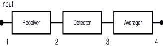
Figure 1: The principal parts of a receiver. In the text, $v_{1}$ is at point 1, $v_{2}$ at point 2, etc.

It has been found that both source and receiver noise has a gaussian distributionRW4 . We assume that the signal is a Gaussian random variable with mean zero

$$p(x)=\frac{1}{\sigma\sqrt{\displaystyle 2\pi}}{\rm\,e}^{-x^{2}/2\sigma^{2}}\,.$$ (41)

which is sampled at a rate equal to twice the bandwidth.

Refer to Fig. 1. By assumption $E(v_{1})=0$. The input, $v_{1}$ has a much larger bandwidth, $B$, than the bandwidth of the receiver, that is, $\mbox{\greeksym{D}}\nu\ll B$.The output of the receiver is $v_{2}$, with a bandwidth $\mbox{\greeksym{D}}\nu$. The power corresponding to the voltage $v_{2}$ is $\left\langle{}v_{2}^{2}\right\rangle$.

$$P_{2}=v_{2}^{2}=\sigma^{2}=k\,T_{\rm sys}\,G\mbox{\greeksym{D}}\nu\;,$$ (42)

where $\mbox{\greeksym{D}}\nu$ is the receiver bandwidth, $G$ is the gain, and $T_{\rm sys}$ is the total noise from the input $T_{\rm A}$ and the receiver $T_{\rm R}$. The contributions to $T_{\rm A}$ are the external inputs from the source, ground and atmosphere. Given that the output of the square law detector is $v_{3}$

$$\left\langle{}v_{3}\right\rangle=\left\langle{}v_{2}^{2}\right\rangle$$ (43)

then after square-law detection we have

$$\left\langle{}v_{3}\right\rangle=\left\langle{}v_{2}^{2}\right\rangle=\sigma^{2}=kT_{\rm sys}G\mbox{\greeksym{D}}\nu\;.$$ (44)

Crucial to a determination of the noise is the mean value and variance of $\left\langle{}v_{3}\right\rangle$ From (36) the result is

$$\left\langle{}v_{3}^{2}\right\rangle=\left\langle{}v_{2}^{4}\right\rangle=3\left\langle{}v_{2}^{2}\right\rangle$$ (45)

this is needed to determine $\left\langle{}\sigma_{3}^{2}\right\rangle$. Then,

$$\sigma_{3}^{2}=\left\langle{}v_{3}^{2}\right\rangle-\left\langle{}v_{3}\right\rangle^{2}$$ (46)

$\left\langle{}v_{3}^{2}\right\rangle$ is the total noise power (= receiver plus input signal). Using the Nyquist sampling rate, the averaged output, $v_{4}$, is $({1}/{N})\Sigma v_{3}$ where $N=2\mbox{\greeksym{D}}\nu\,\tau$.

From $v_{4}$ and $\sigma_{4}^{2}=\sigma_{3}^{2}/N$, we obtain the result

$$\sigma_{4}=k\mbox{\greeksym{D}}\nu G(T_{\rm A}+T_{\rm R})/\sqrt{\mbox{\greeksym{D}}\nu\,\tau}$$ (47)

We have explicitly separated $T_{\rm sys}$ into the sum $T_{\rm A}+T_{\rm R}$. Finally, we use the calibration procedure in Sect.  3.2.1 to eliminate the term $kG\mbox{\greeksym{D}}\nu$:

$$\framebox{$\displaystyle\frac{\mbox{\greeksym{D}}T}{T_{\rm sys}}=\frac{1}{\displaystyle\sqrt{\mbox{\greeksym{D}}\nu\,\tau}}$}\quad.$$ (48)

The calibration process allows us to specify the receiver output in degrees Kelvin instead of in Watts per Hz. We therefore characterize the receiver quality by the system noise temperature $T_{\rm sys}=T_{\rm A}+T_{\rm R}$.

For a given system, the improvement in the RMS noise cannot be better than as given in Eq. (48). Systematic errors will only increase $\Delta T$, although the time behavior may follow the behavior described by (Eq. 48)DICKE . We repeat for emphasis: $T_{\rm sys}$ is the noise from the entire system. That is, it includes the noise from the receiver, atmosphere, ground, and and the source. Therefore $\Delta T$ is larger for an intense source. Except for some planets, however, this situation is rare in the mm/sub-mm range.

3.2.3 Receiver Stability

Sensitive receivers are designed to achieve a low value for $T_{\rm sys}$. Since the signals received are of exceedingly low power, receivers must also provide sufficient output power. This requires a large receiver gain, so even very small gain instabilities can dominate the thermal receiver noise. Therefore receiver stability considerations are also of prime importance. Great advances have been made in improving receiver stability. However in the mm/sub-mm range, the atmosphere plays an important role. To insure that the noise decreases following Eq. 48, systematic effects from atmospheric and receiver instabilities are minimized. Atmospheric changes are of crucial importance. These can be compensated for by rapidly taking the difference between the measurement of the source of interest and a reference region or a nearby calibration source. Such comparison switched measurements are necessary for all ground based observations. R. H. Dicke was the first to apply comparison switching was first applied to radio astronomical receivers DICKE .

The time spent measuring references or performing calibrations will not contribute to an improvement in the S/N ratio. In fact, the subtraction of two noisy inputs worsens the difference, but are needed to reduce instabilities that give rise to systematic errors. The time $\tau$ is the total time taken for the measurement (i. e. on-source and off-source).

Even for the output of a total power receiver there will be additional noise in excess of that given by (48) since the signals to be differenced are $\mbox{\greeksym{D}}T+T_{\rm sys}$ and $T_{\rm sys}$. This is needed since $\mbox{\greeksym{D}}T<<T_{\rm sys}$. For example, if one-half the total time is spent on the reference, the $\mbox{\greeksym{D}}T$ for difference of on-source minus off-source in (48) is a factor of 2 larger.

4 Practical Receivers

This section is concerned with the practical aspects of receivers that are currently in use GOLDSMITHED , RIEKE , with some background material from RW4 .

4.1 Bolometer Radiometers

Figure 2: A bolometer is represented by the smaller square to the right. The power from an astronomical source, $P_{0}$, raises the temperature of the bolometer element by $\Delta\,T$, which is much smaller than the temperature $T_{0}$ of the heat sink. Heat capacity, ${\cal C}$, is analogous to capacitance. The conductance, ${\cal G}$ is analogous to electrical conductance, $G$, which is $1/R$. The noise performance of bolometers depends critically on the thermodynamic temperature, $T_{0}$, and on the conductance ${\cal G}$. The temperature change causes a change in the voltage drop across the bolometer (the details of the electric circuit are not shown)

The operation of bolometers makes use of the effect that the resistance, $R$, of a material varies with the temperature. When radiation is absorbed by the bolometer material, the temperature varies; this temperature change is a measure of the intensity of the incident radiation. Because this thermal effect is rather independent of the frequency of the radiation absorbed, bolometers are intrinsically broadband devices. Frequency discrimination must be provided by external filters.

The Noise Equivalent Power (NEP) quoted for a bolometer is the input power that doubles the output of this device. The expression for NEP is

$$\framebox{$\displaystyle{\rm NEP}_{\rm ph}=2\varepsilon\,k\,T_{\rm BG}\,\sqrt{\Delta\nu}$}\quad.$$ (49)

Where $\varepsilon$ is the emissivity of the background, and T_BG is temperature of the background. Typical values for ground based bolometers are $\varepsilon=0.5,T_{\rm BG}=300$ K and $\Delta\nu=100$ GHz. For these values $NEP_{\rm ph}=1.3\times 10^{-15}$   Watts Hz^-1/2. With the collecting area of the 30 m IRAM telescope and a 100 GHz bandwidth one can easily detect mJy sources.

4.2 Currently Used Bolometer Systems

Bolometers mounted on ground based radio telescopes are background noise limited, so the only way to substantially increase mapping speed for extended sources is to construct large arrays consisting of many pixels. In present systems, the pixels are separated by 2 beamwidths, because of the size of individual bolometer feeds. The systems which best cancel atmospheric fluctuations are composed of rings of close-packed detectors surrounding a single detector placed in the center of the array. Two large bolometer arrays have produced many significant published results. The first is MAMBO2 (MAx-Planck-Millimeter Bolometer). This is a 117 element array used at the IRAM 30-m telescope. This system operates at 1.3 mm, and provides an angular resolution of 11^′′. The portion of the sky that is measured at one instant is the field of view, (FOV). The FOV of MAMBO2 is 240^′′. The second system is SCUBA (Submillimeter Common User Bolometer Array)HOLLAN . This is used on the James-Clerk-Maxwell (JCMT) 15-m sub-mm telescope at Mauna Kea, Hawaii. SCUBA consists of a 37 element array operating at 0.87 mm, with an angular resolution of 14^′′ and a 91 element array operating at 0.45 mm with an angular resolution of 7.5^′′; both have a FOV of about 2.3^′. The LABOCA (LArge Bolometer CAmera) array operates on the APEX 12 meter telescope. APEX is on the 5.1 km high Chaijnantor plateau, the ALMA site in northern Chile. The LABOCA camera operates at 0.87 mm waqvelength, with 295 bolometer elements. These are arranged in 9 concentric hexagons around a center element. The angular resolution of each element is 18.6^′′, the FOV is 11.4^′. Such an arrangement is ideal for the measurement of small sources since the outer rings of detectors can be used to subtract the emission from the sky, while the central elements are measuring the source.

4.2.1 Superconducting Bolometers

A promising new development in bolometer receivers is Transition Edge Sensors referred to as TES bolometers. These superconducting devices may allow more than an order of magnitude increase in sensitivity, if the bolometer is not background limited. For broadband bolometers used on earth-bound telescopes, the warm background limits the performance. With no background, the noise improvement with TES systems is limited by photon noise; in a background noise limited situation, TES’s should be $\sim$2–3 times more sensitive than semiconductor bolometers. For ground based telescopes, TES’s greatest advantage is multiplexing many detectors with a superconducting readout device, so one can construct even larger arrays of bolometers. SCUBA will be replaced with SCUBA-2 now being constructed at the U. K. Astronomy Technology Center. SCUBA-2 is an array of 2 TES bolometers, each consisting of 6400 elements operating at 0.87 mm and 0.45 mm. The FOV of SCUBA-2 will be 8^′. The SCUBA-2 design is based on photo-deposition technology similar to that used for integrated circuits. This type of construction allows for a closer packing of the individual bolometer pixels. In SCUBA-2 these will be separated by 1/2 of a beam, instead of the usual 2 beam spacing.

4.2.2 Polarization & Spectral Line Measurements

In addition to measuring the continuum total power, one can mount a polarization-sensitive device in front of the bolometer and thereby measure the direction and degree of linear polarization. These devices have been used with SCUBA on the James-Clerk-Maxwell Telescope in Hawaii and (in the past) with a 19 beam bolometer at the Heinrich-Hertz-Telescope in Arizona.

It is possible to also carry out spectroscopy, if frequency sensitive elements, either Michelson or Fabry-Perot interferometers, are placed before the bolometer element. Since these spectrometers operate at the sky frequency, the fractional resolution ($\mbox{\greeksym{D}}\nu/\nu$) is limited.

4.3 Coherent Receivers

Coherent receivers are those which preserve the phase of the signal. Usually, coherent receivers make use of the superheterodyne (or more commonly ^′′heterodyne^′′) principle to shift the signal input frequency without changing other properties; in practice, this is carried out by the use of mixers (Section 4.3.3). Heterodyne is commonly used in all branches of communications technology; its use allows measurements with unlimited spectral resolution, $\Delta\nu/\nu$.

4.3.1 The Minimum Noise in a Coherent System

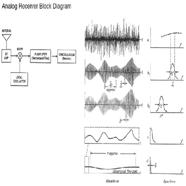
Figure 3: On the left are the parts of a coherent receiver. For $\nu_{0}<$120 GHz one can amplify before mixing while for higher frequencies the first circuit element is the mixer. In the middle are sketches of the time behavior of broadband noise after passing through these parts of the receiver; on the right are sketches of the corresponding frequency behavior. The mixer shifts the signal to a lower freuqency while the amplifier increases the output over a narrow band. The square law detector converts rapidly oscillating signals into a smooth response that has positive values. The middle and right sketches are taken from PAWSEY .

The ultimate limit for coherent receivers or amplifiers is obtained by application of the Heisenberg uncertainty principle. The $minimum$ noise of a coherent amplifier results in a receiver noise temperature of

$$\framebox{$\displaystyle T_{\rm rx}({\rm minimum})=\frac{h\nu}{k}$}\quad.$$ (50)

For incoherent detectors, such as bolometers, phase is not preserved, so this limit does not exist. In the millimeter wavelength regions, this noise temperature limit is quite small. At $\lambda$=2.6 mm ($\nu$=115 GHz), this limit is 5.5 K.

4.3.2 Elements of Coherent Receivers

The noise in the first element dominates the system noise. The exact expression is given by the Friis relation which takes into account the effect of having cascaded amplifiers :

$$\framebox{$\displaystyle T_{\rm S}=T_{\rm S1}+\frac{1}{G_{1}}T_{\rm S2}+\frac{1}{G_{1}G_{2}}T_{\rm S3}+\dots+\frac{1}{G_{1}G_{2}\dots G_{n-1}}T_{{\rm S}n}$}\quad.$$ (51)

Where $G_{1}$ is the gain of the first element, and $T_{\rm S1}$ is the noise temperature of this element. The corresponding values apply to the following elements in a receiver. For $\lambda<$3 mm, cooled first elements typically have $G_{1}=10^{3}$ and $T_{\rm S1}=50$K; for $\lambda<$0.3 mm, cooled first elements typically have $G_{1}=1$ and $T_{\rm S1}=500$K.

4.3.3 Mixers

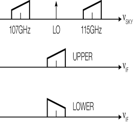
Figure 4: A sketch of the frequencies shifted from the sky frequency (top) to the output (lower) of a double sideband mixer. In this example, the input is at the sky frequencies for the Upper Side Band (USB) of 115 GHz, and Lower Side Band (LSB) of 107 GHz while the output frequency is 4 GHz. The slanted boxes represent the passbands; the direction of the slant in the boxes indicate the upper (higher) and lower (lower) edge of the bandpass in frequency RW5 . ALMA mm mixers are SSB mixers so these effects are avoided.

Mixers allow the signal frequency to be changed without altering the characteristics of the signal. In the mixing process, one multiplies the input signal with an intense monochromatic signal from a local oscillator, LO, in a non-linear circuit element. In principle a mixer produces a shift in frequency of an input signal with no other effect on the signal properties. For a single mixer, two frequency bands, at equal separations from the LO frequency are shifted into intermediate (IF) frequency band. This is Double Sideband (DSB) mixer operation. These are referred to as the signal and image bands. In the mm/sub-mm wavelength ranges, such mixers are still commonly used as the first stage of a receiver. For single dish continuum measurements, both sidebands contain the signal, so DSB operation does not decrease the signal-to-noise (S/N) ratio. However, for single dish spectral line measurements, the spectral line of interest is in one sideband only. The other sideband is then a source of extra noise (i. e. lower S/N ratio) and perhaps confusing lines. Therefore single sideband (SSB) operation is desired. If the image sideband is eliminated, the mixer is said to operate in SSB mode. This can be accomplished by inserting a filter before the mixer. However, filters cause a loss of signal, so lower the S/N ratio. For low noise applications a more complex arrangement is needed. In many cases, a single sideband mixer is used. This consists of two identical mixers driven by a single local oscillator through a phase shifting device.

For example, the ALMA Band 7 mm/sub-mm receiver shifts a signal centered at 345 GHz from the sky frequency, 341 to 349 GHz to 4-12 GHz. At 4 to 12 GHz the signal is easily amplified. This is an SSB mixer; the unwanted sideband is not accepted.

Noise in mixers has 3 causes. The first is the mixer itself. Since one half of the input signal at $\nu_{\rm sky}$ is shifted to an unwanted frequency $\nu_{\rm LO}+\nu_{\rm sky}$, the signal suffers a factor-of-two (3 db) loss. This is referred to as conversion loss.Classical mixers typically have 3 db (=factor of 2) loss. In Eq. 51, $G_{1}=1/2$. In addition there will be an additional noise contribution from the mixer itself ( $T_{\rm S1}$ in (51)). Second, the LO may have ^′′phase noise^′′, that is a rapid change of phase, which will affect signal properties, so adds to the uncertainties. Third, the amplitude of the LO may vary. This effect can be minimized since the mixer LO power is adjusted so that the mixer output is saturated. Then there is no variation of the output signal power if LO power varies.

4.4 HEMTs/MMICs

Within a highly ordered crystal made of identical atoms, free electrons can move only within certain energy bands. By varying the material, both the width of the band, the band gap, and the energy to reach a conduction band can be varied. The crucial part of any semiconductor device is the junction. On the one side there is an excess of material with negative carriers, forming n-type material and the other side material with a deficit of electrons, that is p-type material. The p-type material has an excess of positive carriers, or holes. At the junction of a p- and n-type material, the electrons in the n-type material can diffuse into the p-type material (and vice-versa), so there will be a net potential difference. The diffusion of charges, p to n and n to p, cannot continue indefinitely, but a difference in the charges near the boundary of the n and p material will remain, because of the low conductivity of the semiconductor material. From the potential difference at the junction, a flow of electrons in the positive direction is easy, but a flow in the negative direction will be hindered. Typical p-n junctions have a slow response so are suitable only as square-law detectors. Schottky (metal-semiconductor) junctions have a lower capacitance, so are better suited to applications such as microwave mixers. The combination of three layers, p-n-p, in a so-called ^′′sandwich^′′, is a simple extension of the p-n junction. In Field Effect Transistors, FET’s, the electric field controls the carrier flow so this is an amplifier. At frequencies of 100 GHz, unipolar devices, which have only one type of carrier, are used as microwave amplifier front ends. High Electron Mobility Transistors, HEMTs, are an evolution of FETs. The design goals of HEMT’s are: (1) to obtain lower intrinsic amplifier noise and (2) operation at higher frequency. In HEMTs, the charge carriers are present in a channel of small size. This confinement gives rise to a two dimensional electron gas, or ^′′2 DEG^′′, where there is less scattering and hence lower noise. When cooled, there is a significant improvement in the noise performance, since the main contribution is from the oscillations of nuclei in the lattice, which are strongly temperature dependent. To extend the operation of HEMT to higher frequencies, one must increase electron mobility, $\mu$, and saturation velocity $V_{\rm s}$. A reduction in the scattering by introducing impurities (^′′doping^′′) leads to a larger electron mobility, $\mu$, and hence faster transit times, in addition to lower amplifier noise.

For use up to $\nu$=115 GHz with good noise performance, one has turned to modifications of HEMTs based on advances in material-growth technology. The SEQUOIA receiver array of the Five College Radio Astronomy Observatory uses Microwave Monolithic Integrated Circuits (MMIC’s) in 32 front ends for a 16 beam, two polarization system (pioneered by S. Weinreb). The MMIC is a complete amplifier on a single semiconductor, instead of using lumped components. The MMIC’s have excellent performance in the 80–115 GHz region without requiring tuning adjustments. The simplicity makes MMIC’s better suited for multi-beam systems.

For low noise IF amplifiers, 4 to 8 GHz IF systems using Gallium-Arsinide HEMTs with 5 K noise temperature and more than 20 db of gain have been built. With Indium-Phosphide HEMTs on GaAs-substrates, even lower noise temperatures are possible. As a rule of thumb, one expects an increase of 0.7 K per GHz for GaAs, while the corresponding value for InP HEMTs is 0.25 K per GHz. For front ends, noise temperatures of the amplifiers in the 18–26 GHz range are typically 12 K.

4.4.1 Superconducting Mixers

Very general, semi-classical considerations indicate that the slope of the current-voltage, $I$-$V$, curve for classical mixers changes gently. This leads to a relatively poor noise figure for classical mixers, since much of the input signal is not converted to a lower frequency.

A significant improvement can be obtained if the junction is operated in the superconducting mode. Then the gap between filled and empty states is comparable to photon energies in the mm/sub-mm range. In addition, the LO power requirements are $\approx 1000$ times lower than are needed for conventional mixers. Finally, the physical layout of such devices is simpler since the mixer is a planar device, deposited on a substrate by lithographic techniques. SIS mixers consist of a superconducting layer, a thin insulating layer and another superconducting layer. SIS mixers depend on single carriers; a longer but more accurate description of SIS mixers is ^′′single quasiparticle photon assisted tunneling detectors^′′. When the SIS junction is properly biased, the filled states reach the level of the unfilled band, and the electrons can quantum mechanically tunnel through the insulating strip. The $I$-$V$ curve for a SIS device shows sudden jumps in the $I$-$V$ curve; these are typical of quantum-mechanical phenomena. For low noise operation, the SIS mixer must be DC biased at an appropriate voltage and current. If, in addition to the mixer bias, there is a source of photons of energy $h\nu$, then the tunneling can occur. If one then biases an SIS device and applies an LO signal at a frequency $\nu$, the $I$-$V$ curve becomes very sharp, so the conversion of sky signals to the IF frequency is much more effective than with a classical mixer.

Under certain circumstances, SIS devices can produce gain. If the SIS mixer is tuned to produce substantial gain, it is unstable. Thus, this not useful in radio astronomical applications. In the mixer mode, that is, as a frequency converter, SIS devices can have a small amount of gain. This tends to balance inevitable mixer losses, so SIS devices have losses that are lower than classical mixers. SIS mixers have performance that is unmatched in the mm/sub-mm region. In addition to single sideband properties, improvements to existing designs include tunerless and SIS mixers. Tunerless mixers have the advantage of repeatability in tuning. For ALMA, SIS mm mixer designs are wideband, tunerless, single sideband devices with extremely low mixer noise temperatures.

An increase in the gap energy is needed to allow the efficient mixing at higher frequenccies. This is done with Niobium superconducting materials; the geometric junction sizes are $1\thinspace\mbox{\greeksym{m}}$m by $1\thinspace\mbox{\greeksym{m}}$m. For frequencies above 900 GHz, one uses niobium nitride junctions. Variants of such devices, such as the use of junctions in series, can be used to reduce the capacitance. An alternative is to reduce the size of the individual junctions to $0.25\thinspace\mbox{\greeksym{m}}$m.

SIS mixers are the front ends of choice for operation between 150 GHz and 900 GHz because these are low-noise devices, the IF bandwidths can be $>$1 GHz, these are tunable over $\sim$30% of the frequency range and the local oscillator power needed is $<$1 $\mbox{\greeksym{m}}{\rm W}$.

4.4.2 Hot Electron Bolometers

Superconducting Hot Electron Bolometer-mixers (HEB) are heterodyne devices, in spite of the name. These mixers make use of superconducting thin films which have sub-micron sizes. In an HEB mixer excess noise is removed either by diffusion of hot electrons out the junction, or by an electron-phonon exchange. The first HEBs operating on radio telescopes and used to take astronomical made use of electron-phonon exchange. The HEB junctions were of $\umu$m size, consisting of Niobium Nitride (NbN), cooled to 4.2 K. Junctions of Aluminum-Titanium-Nitride, AlTiN, have provided lower receiver noise temperatures. The IF center frequency was 1.8 GHz, and a had a full width of 1 GHz. Such a system was used to measure the $J=9-8$ carbon monoxide line at 1.037 THz. Later, the group of First Physical Institute at Cologne University used the Atacama Pathfinder EXperiment (APEX) telescope to measure the [N II] line at 1.5 THz (see Table 1).

4.4.3 Single Pixel Receiver Systems

In summary, devices that provide the lowest noise front ends are:

for $\nu<115$ GHz, High Electron Mobility Transistors (HEMT) and Microwave Monolithic Integrated Circuits (MMIC)

for $72<\nu<800$ GHz, Superconducting Mixers (SIS)

for $\nu>900$ GHz, Hot Electron Bolometers (HEB)

SIS mixers provide the lowest receiver noise in the mm and sub-mm range. SIS mixers are much more sensitive than classical Schottky mixers, and require less local oscillator power, but must be cooled to 4 Kelvin. All millimeter mixer receivers are tunable over 10 to 20 % of the sky frequency. From the band gaps of junction materials, there is a short wavelength limit to the operation of SIS devices. For spectral line measurements at wavelengths, at $\lambda<0.3$ mm, superconducting Hot Electron Bolometers (HEB), which have no such limit, have been developed. At frequencies above 2 THz there is a transition to far-infrared and optical techniques. The highest frequency heterodyne systems in radio astronomy are used in the Herschel-HIFI satellite. These are SIS and HEB mixers.

The SIS or HEB mixers convert the sky frequency to the fixed IF frequency, where the signal is amplified by the IF amplifiers. Most of the amplification is done in the IF. The IF should only contribute a negligible part to the system noise temperature. Because some losses are associated with frequency conversion, the first mixer is a major source for the system noise. Two ways exist to decrease this contribution: (1) by use of either an SIS or HEB mixer to convert the input to a lower frequency, or (2) at lower frequencies by use of a low-noise amplifier before the mixer.

4.4.4 Multibeam Systems

At 3 mm, the SEQUOIA array receiver produced at the Five College Radio Astronomy Observatory (FCRAO) with 32 MMIC front ends connected to 16 beams had been used on 14-m telescope of the FCRAO for the last few years. Multibeam system that use SIS front ends are rare. A 9 beam Heterodyne Receiver Array of SIS mixers at 1.3 mm, HERA, has been installed on the IRAM 30-m millimeter telescope to measure spectral line emission. To simplify data taking and reduction, the HERA beams are kept on a Right Ascension-Declination coordinate frame. HARP-B is a 16 beam SIS system in operation at the James-Clerk-Maxwell telescope. The sky frequency is 325 to 375 GHz. The beam size of each element is 14^′′, with a beam separation of 30^′′, and a FOV of about 2^′. The total number of spectral channels in a heterodyne multi-beam system will be large. In addition, complex optics is needed to properly illuminate all of the beams. In the mm range this usually means that the receiver noise temperature of each element is somewhat larger than that for a single pixel receiver system. For further details of SEQUOIA, HERA or HARP, see the appropriate web sites.

For single dish continuum measurements at $\lambda<$ 2 mm, multi-beam systems make use of bolometers. GeGa bolometers are the most common systems and the best such systems have a large number of beams. In the future, TES bolometers seem to have great promise. Compared to incoherent recievers, heterodyne systems are still the most efficient for spectral lines in the range $\lambda>$0.3mm, although Fabry-Perot systems (such as SPIFI; see the web site) may be competitive for some projects. For bolometers on the Herschel satellite, one uses gratings or Fabry-Perot systems. For SCUBA-2, an analog Michelson ( Fourier transform interferometer) is proposed.

4.5 Back Ends: Spectrometers

The term ^′′Back End^′′ is used to specify the devices following the IF amplifiers. Of the many different back ends that have been designed for specialized purposes, spectrometers are probably the most widely used. Previously this was carried out in especially designed hardware, but recently there have been devices based on general purpose digital computers.

Spectrometers analyze the spectral information contained in the radiation field. To accomplish this these must be SSB and the frequency resolution $\Delta\nu$ is usually fine; perhaps in the kHz range. In addition, the time stability must be high. If a resolution of $\Delta\nu$ is to be achieved for the spectrometer, all those parts of the system that enter critically into the frequency response have to be maintained to better than $0.1\,\Delta\nu$. An overview of the current state of spectrometers is to be found in BAKER .

4.5.1 Multichannel Filter Spectrometers

The time needed to measure the power spectrum for a given celestial position can be reduced by a factor $n$ if the IF section with the filters defining the bandwidth $\Delta\nu$, the square-law detectors and the integrators are built not merely once, but $n$ times. Then these form $n$ separate channels that simultaneously measure different (usually adjacent) parts of the spectrum.

4.6 Fourier, Autocorrelation and Cross Correlation Spectrometers

One method is to Fourier Transform (FT) the input, $v(t)$, to obtain $v(\nu)$ and then square $v(\nu)$ to obtain the Power Spectral Density. From the Nyquist theorem, it is necessary to sample at a rate equal to twice the bandwidth. These are referred to as ^′′FX^′′ autocorrelators. Recent developments at the Jodrell Bank Observatory have led to the building of COBRA (Coherent Baseband Receiver for Astronomy). COBRA can analyze a 100 MHz bandwidth. A similar device with a 1 GHz bandwidth has been built at the Max-Planck-Institut in Bonn for use in the mm/sub-mm range on APEX.

For Autocorrelators, or XF systems, the input $v(t)$ is correlated with a delayed signal $v(t-\tau)$ to obtain the autocorrelation function $R(\tau)$ function. $R(\tau)$ is then Fourier Transformed to obtain the spectrum. For an XF system the time delays are performed in a set of serial digital shift registers with a sample delayed by a time $\tau$. Autocorrelation can also be carried out with the help of analog devices using a series of cable delay lines. Such analog correlators have been developed at the University of Maryland together with NRAO for use on the Green Bank Telescope (GBT); these are used to provide very large bandwidths.

The two significant advantages of digital spectrometers are: (1) flexibility and (2) a noise behavior that follows $1/\sqrt{t}$ after many hours of integration. The flexibility allows one to select many different frequency resolutions and bandwidths or even to employ a number of different spectrometers, each with different bandwidths, simultaneously. The second advantage follows directly from their digital nature. Once the signal is digitized, it is only mathematics. Tests on astronomical sources have shown that the noise follows a ${1}/{\sqrt{Bt}}$ behavior for integration times $>$100 hours; in these aspects, analog spectrometers are more limited.

A serious drawback of digital auto and cross correlation spectrometers had been limited bandwidths. Previously 50 to 100 MHz had been the maximum possible bandwidth. This was determined by the requirement to meet Nyquist sampling rate, so that the analog-to-digital (A/D) converters, samplers, shift registers and multipliers would have to run at a rate equal to twice the bandwidth. The speed of the electronic circuits was limited. However, advances in digital technology in recent years have allowed the construction of autocorrelation spectrometers with several 1000 channels covering bandwidths of several GHz.

Another improvement is the use of recycling auto and cross correlators. These spectrometers have the property that the product of bandwidth, $B$ times the number of channels, $N$, is a constant. Basically, this type of system functions by having the digital part running at a high clock rate, while the data are sampled at a much slower rate. Then after the sample reaches the $N$th shift register it is reinserted into the first register and another set of delays are correlated with the current sample. This leads to a higher number of channels and thus higher resolution. Such a system has the advantage of high-frequency resolution, but is limited in bandwidth. This has the greatest advantage for longer wavelength observations. Both of these developments have tended to make the use of digital spectrometers more widespread. This trend is likely to continue.

Autocorrelation systems are used in single telescopes, and make use of the symmetric nature of the autocorrelation function ACF. Thus, the number of delays gives the number of spectral channels. For cross-correlation, the current and delayed samples refer to different inputs. Cross-correlation systems are used in interferometers. In the simplest case of a two-element interferometer, the output is not symmetric about zero time delay, but can be expressed in terms of amplitude and phase at each frequency, where both the phase and intensity of the line signal are unknown. Thus, for interferometry the zero delay of the ACF is placed in channel $N/2$ and is in general asymmetric. The number of delays, $N$, allows the determination of $N/2$ spectral intensities, and $N/2$ phases. The cross-correlation hardware can employ either an XF or a FX correlator. The FX correlator has the advantage that the time delay is just a phase shift, so can be introduced more simply.

4.6.1 Acousto-Optical Spectrometers

Since the discovery of molecular line radiation in the mm wavelength range there has been a need for spectrometers with bandwidths of several GHz. At 100 GHz, a velocity range of 300 km s^-1 corresponds to 100 MHz, while the narrowest line widths observed correspond to 30 kHz. Autocorrelation spectrometers can reach such large bandwidths only if complex methods are used. The AOS makes use of the diffraction of light by ultrasonic waves: these cause periodic density variations in the medium through which it passes. These density variations in turn cause variations in the bulk constants $\varepsilon$ and $n$ of the medium, so that a plane electromagnetic wave passing through this medium will be affected. The most advanced AOS’s have been designed and built at the First Physical Institute at Cologne University.

5 Filled Aperture Antennas

The material presented in the following emphasizes descriptive antenna parameters. These allow a fairly accurate but rather simple description of antenna properties that are needed for an accurate interpretation of astronomical measurements. For more detail, see BAARS . An important concept is reciprocity, in which the properties of antennas are the same, irrespective whether these are used for receiving or transmitting. Reciprocity is limited under some (very special) circumstances that are not encountered in astronomy.

5.1 Angular Resolution

From diffraction theory JENKINS , the angular resolution of a reflector of diameter $D$ at a wavelength $\lambda$ is

$$\framebox{$\displaystyle\theta=\frac{\lambda}{D}$}\quad.$$ (52)

This simple result gives an approximate value for $\theta$ but more detailed results must take into account details of the illumination.

5.2 The Power Pattern $P(\vartheta,\varphi)$

Often, the normalized power pattern, not the power pattern is measured:

$$\framebox{$\displaystyle P_{\rm n}(\vartheta,\varphi)=\frac{1}{P_{\rm max}}\,P(\vartheta,\varphi)$}\quad.$$ (53)

The reciprocity theorem provides a method to measure this quantity. The radiation source can be replaced by a small diameter radio source. The flux densities of such sources are determined by measurements using horn antennas at centimeter and millimeter wavelengths. At short wavelengths, one uses planets, or moons of planets, whose surface temperatures are determined from infrared data.

If the power pattern is measured using artificial transmitters, care should be taken that the distance from a large antenna A (diameter $D$) to a small antenna B (transmitter) is so large that B produces plane waves across the aperture $D$ of antenna A, i. e. is in the far radiation field of A. This is the Rayleigh distance; it requires that the curvature of a wavefront emitted by B is much less than a wavelength across the geometric dimensions of A. This curvature must be $k\ll 2D^{2}/\lambda$, for an antenna of diameter $D$ and a wavelength $\lambda$.

Consider the power pattern of the antenna used as a transmitter. If the spectral power density, $\mathcal{P}_{\nu}$ in [W Hz^-1] is fed into a lossless isotropic antenna, this would transmit $P$ power units per solid angle per Hertz. Then the total radiated power at frequency $\nu$ is $4\pi\,P_{\nu}$ In a realistic, but still lossless antenna, a power $P(\vartheta,\varphi)$ per unit solid angle is radiated in the direction $(\vartheta,\varphi)$. If we define the directive gain $G(\vartheta,\varphi)$ as the

$$P(\vartheta,\varphi)=G(\vartheta,\varphi)\,P$$

or

$$\framebox{$\displaystyle G(\vartheta,\varphi)=\displaystyle\frac{4\pi P(\vartheta,\varphi)}{\int\!\!\int P(\vartheta,\varphi)\,{\rm\,d}\Omega}$}\quad.$$ (54)

Thus the gain or directivity is also a normalized power pattern similar to (53), but with the difference that the normalizing factor is $\int P(\vartheta,\varphi){\rm\,d}\Omega/4\pi$. This is the gain relative to a lossless isotropic source. Since such an isotropic source cannot be realized in practice, a measurable quantity is the gain relative to some standard antenna such as a half-wave dipole whose directivity is known from theoretical considerations.

5.3 The Main Beam Solid Angle

Figure 5: A polar power pattern showing the main beam, and near and far side lobes. The weaker far side lobes have been combined to form the stray pattern

The beam solid angle $\Omega_{\rm A}$ of an antenna is given by

$$\framebox{$\displaystyle\Omega_{\rm A}=\parbox{22.76219pt}{$\vspace*{-2mm}{\displaystyle\int\!\!\int\atop{\!\!\!\!\!\scriptstyle 4\pi}}$ }P_{\rm n}(\vartheta,\varphi)\,{\rm\,d}\Omega=\int\limits_{0}^{2\pi}\!\int\limits_{0}^{\pi}P_{\rm n}(\vartheta,\varphi)\sin\vartheta{\rm\,d}\vartheta{\rm\,d}\varphi$}$$ (55)

this is measured in steradians (sr). The integration is extended over the full sphere $4\pi$, such that $\Omega_{\rm A}$ is the solid angle of an ideal antenna having $P_{\rm n}=1$ for all of $\Omega_{\rm A}$ and $P_{\rm n}=0$ everywhere else. Such an antenna does not exist; for most antennas the (normalized) power pattern has considerably larger values for a certain range of both $\vartheta$ and $\varphi$ than for the remainder of the sphere. This range is called the main beam or main lobe of the antenna; the remainder are the side lobes or back lobes (Fig. 5). For actual situations, the properties are well defined up to the the shortest operating wavelengths. At the shortest wavelength, there is still a main beam, but much of the power enters through sidelobes. In addition, the main beam efficiency may vary significantly with elevation and weather has a large effect. Thus, the ability to accurately calibrate the radio telescope at sub-mm wavelengths is challenging.

In analogy to (55) we define the main beam solid angle $\Omega_{\rm MB}$ by

$$\framebox{$\displaystyle\Omega_{\rm MB}=\mathop{\int\!\!\int}\limits_{\scriptstyle\rm main\atop\scriptstyle\rm lobe}P_{\rm n}(\vartheta,\varphi)\,{\rm\,d}\Omega$}\quad.$$ (56)

The quality of an antenna as a direction measuring device depends on how well the power pattern is concentrated in the main beam. If a large fraction of the received power comes from the side lobes it would be rather difficult to determine the location of the radiation source, the so-called ^′′pointing^′′.

It is appropriate to define a main beam efficiency or (in the slang of antenna specialists) beam efficiency, $\eta_{\rm B}$, by

$$\framebox{$\displaystyle\eta_{\rm B}=\frac{\Omega_{\rm MB}}{\Omega_{\rm A}}$}\quad.$$ (57)

The main beam efficiency, $\eta_{\rm B}$ is the fraction of the power is concentrated in the main beam. The main beam efficiency can be modified (within certain limits) for parabolic antennas by the illumination of the main reflector. If the FWHP beamwidth is well defined, the location of an isolated source is determined to an accuracy given by the FWHP divided by the S/N ratio. Thus, it is possible to determine positions to small fractions of the FWHP beamwidth if noise is the only limit.

Substituting (55) into (54) it is easy to see that the maximum directive gain $G_{\rm max}$ or directivity $\cal D$ can be expressed as

$$\framebox{$\displaystyle{\cal D}=G_{\rm max}=\frac{4\pi}{\Omega_{\rm A}}$}\quad.$$ (58)

The angular extent of the main beam is usually described by the half power beam width (HPBW), which is the angle between points of the main beam where the normalized power pattern falls to $1/2$ of the maximum. For elliptically shaped main beams, values for widths in orthogonal directions are needed. The beamwidth is related to the geometric size of the antenna and the wavelength used; the exact beamsize depends on details of illumination.

5.4 Effective Area

Let a plane wave with the power density $\mid\!\langle\vec{S}\rangle\!\mid$ be intercepted by an antenna. A certain amount of power is then extracted by the antenna from this wave; let this amount of power be $P_{\rm e}$. We will then call the fraction

$$A_{\rm e}=P_{\rm e}\,/\mid\!\langle\vec{S}\rangle\!\mid$$ (59)

the effective aperture of the antenna. $A_{\rm e}$ has the dimension of m². Comparing this to the geometric aperture $A_{\rm g}$ we can define an aperture efficiency $\eta_{\rm A}$ by

$$\framebox{$\displaystyle A_{\rm e}=\eta_{\rm A}A_{\rm g}$}\quad.$$ (60)

Consider a receiving antenna with a normalized power pattern $P_{\rm n}(\vartheta,\varphi)$ that is pointed at a brightness distribution $B_{\nu}(\vartheta,\varphi)$ in the sky. Then at the output terminals of the antenna, the total power per unit bandwidth, $\cal{P}_{\nu}$ is

$$\mathcal{P}_{\nu}={\textstyle\frac{1}{2}}\,A_{\rm e}\int\!\!\int B_{\nu}(\vartheta,\varphi)\,P_{\rm n}(\vartheta,\varphi)\,{\rm\,d}\Omega\;.$$ (61)

By definition, we are in the Rayleigh-Jeans limit, and can therefore exchange the brightness distribution by an equivalent distribution of brightness temperature. Using the Nyquist theorem (28) we can introduce an equivalent antenna temperature $T_{\rm A}$ by

$$\mathcal{P}_{\nu}=k\,T_{\rm A}\,.$$ (62)

This definition of antenna temperature relates the output of the antenna to the power from a matched resistor. When these two power levels are equal, then the antenna temperature is given by the temperature of the resistor. Instead of the effective aperture $A_{\rm e}$ we can introduce the beam solid angle $\Omega_{\rm A}$. Then (61) becomes

$$T_{\rm A}(\vartheta_{0},\varphi_{0})=\frac{\int T_{\rm B}(\vartheta,\varphi)P_{\rm n}(\vartheta-\vartheta_{0},\varphi-\varphi_{0})\sin\vartheta{\rm\,d}\vartheta{\rm\,d}\varphi}{\int P_{\rm n}(\vartheta,\varphi){\rm\,d}\Omega}$$ (63)

which is the convolution of the brightness temperature with the beam pattern of the telescope. The brightness temperature $T_{\rm b}(\vartheta,\varphi)$ corresponds to the thermodynamic temperature of the radiating material only for thermal radiation in the Rayleigh-Jeans limit from an optically thick source; in all other cases $T_{\rm B}$ is only an convenient quantity that in general depends on the frequency. It is important to note that from (63), the measured size of an extremely compact (i. e. “point”) source is the beam size.

The quantity $T_{\rm A}$ in (63) was obtained for an antenna with no ohmic losses, and no absorption in the earth’s atmosphere. In the mm/sub-mm range, the expression $T_{\rm A}$ in (63) is actually $T_{\rm A}^{\prime}$, that is, a temperature corrected for atmospheric losses. We will use the term $T_{\rm A}^{\prime}$ in discussions of mm/sub-mm calibration. Since $T_{\rm A}$ is the quantity measured while $T_{\rm B}$ is the one desired, (63) must be inverted. (63) is an integral equation of the first kind, which in theory can be solved if the full range of $T_{\rm A}(\vartheta,\varphi)$ and $P_{\rm n}(\vartheta,\varphi)$ are known. In practice this inversion is possible only approximately. Usually both $T_{\rm A}(\vartheta,\varphi)$ and $P_{\rm n}(\vartheta,\varphi)$ are known only for a limited range of $\vartheta$ and $\varphi$ values, and the measured data are not free of errors. Therefore usually only an approximate deconvolution is performed. A special case is one for which the source distribution $T_{\rm B}(\vartheta,\varphi)$ has a small extent compared to the telescope beam. Given a finite signal-to-noise ratio, the best estimate for the upper limit to the actual FWHP source size is one-half of the FWHP of the telescope beam. This point cannot be emphasized too much: we cannot assign an arbitrarily small size to a source. The best is one-half of the antenna FWHP!

5.5 Antenna Feed Horns Used Today

Feed horns are needed to guide the power from the reflector (in free space conditions) into the receiver (in a waveguide); details are contained in GOLDSMITH ,LOVE . The electric and magnetic field strengths at the open face of a wave guide will vary across the aperture. The power pattern of this radiation depends both on the dimension of the wave guide in units of the wavelength, $\lambda$, and on the mode of the wave. The greater the dimension of the wave guide in $\lambda$, the greater is the directivity of this power pattern. However, the larger the cross-section of a wave guide in terms of the wavelength, the more difficult it becomes to restrict the wave to a single mode. Thus wave guides of a given size can be used only for a limited frequency range. The aperture required for a selected directivity is then obtained by flaring the sides of a section of the wave guide so that the wave guide becomes a horn.

Great advances in the design of feeds have been made since 1960, and most parabolic dish antennas now use hybrid mode feeds. Such ^′′corregated horns^′′ are also referred to as Scalar or Multi-Mode feeds. Today such feed horns are used on all parabolic antennas. These provide much higher efficiencies than simple single mode horns and are well suited for polarization measurements.

5.6 Multiple Reflector Systems

If the size of a radio telescope is more than a few hundred wavelengths, designs similar to those of optical telescopes are preferred. For such telescopes Cassegrain, Gregorian and Nasmyth systems have been used. In a Cassegrain system, a convex hyperbolic reflector is introduced into the converging beam immediately in front of the prime focus. This reflector transfers the converging rays to a secondary focus which, in most practical systems is situated close to the apex of the main dish. A Gregorian system makes use of a concave reflector with an elliptical profile. This must be positioned behind the prime focus in the diverging beam. In the Nasmyth system this secondary focus is situated in the elevation axis of the telescope by introducing another, usually flat, mirror. The advantage of a Nasmyth system is that the receiver front ends remain horizontal while when the telescope is pointed toward different elevations. This is an advantage for receivers cooled with liquid helium, which may become unstable when tipped. Cassegrain and Nasmyth foci are commonly used in the mm/sub-mm wavelength ranges.

In a secondary reflector system, feed illumination beyond the edge receives radiation from the sky, which has a temperature of only a few K. For low-noise systems, this results in only a small overall system noise temperature. This is significantly less than for prime focus systems. This is quantified in the so-called ^′′G/T value^′′, that is, the ratio of antenna gain of to system noise. Any telescope design must aim to minimize the excess noise at the receiver input while maximizing gain. For a specific antenna, this maximization involves the design of feeds and the choice of foci.

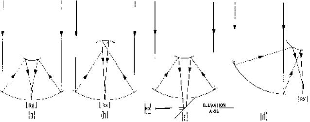
Figure 6: The geometry of (a) Cassegrain, (b) Gregorian, (c) Nasmyth and (d) offset Cassegrain systems (from RW4 ).

That the secondary reflector blocks the central parts in the main dish from reflecting the incoming radiation causes some interesting differences between the actual beam pattern from that of an unobstructed telescope. Modern designs seek to minimize blockage due to the support legs and subreflector.

Realistic filled aperture antennas (^′′single dishes^′′) will have a beam pattern different from a uniformly illuminated unblocked aperture. First the illumination of the reflector will not be uniform but has a taper by 10 dB or more at the edge of the reflector. The side-lobe level is strongly influenced by this taper: a larger taper lowers the sidelobe level. Second, the secondary reflector must be supported by three or four support legs, which will produce aperture blocking and thus affect the shape of the beam pattern. In particular feed leg blockage will cause deviations from circular symmetry. For altitude-azimuth telescopes these side lobes will change position on the sky with hour angle. This may be a serious defect, since these effects will be significant for maps of low intensity regions if the main lobe is near an intense source. The side lobe response can also dependent on the polarization of the incoming radiation.

A disadvantage of on-axis systems, regardless of focus, is that they are often more susceptible to instrumental frequency baselines, so-called baseline ripples across the receiver band than primary focus systems. Part of this ripple is caused by multiple reflections of noise from source or receiver in the antenna structure. Ripples can arise in the reciever, but these can be removed or compensated rather easily. Telescope baseline ripples are more difficult to eliminate: it is known that large amounts of blockage and larger feed sizes lead to large baseline ripples. The effect is discussed in somewhat more detail in Sect. 6.4. The influence of baseline ripples on measurements can be reduced to a limited extent by appropriate observing procedures. A possible solution is the construction of off-axis systems such as the GBT.

5.7 Antenna Tolerance Theory

It is convenient to distinguish several different kinds of phase errors in the current distribution across the aperture of a two-dimensional antenna.

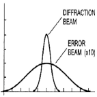
Figure 7: A sketch showing the relative widths of the main beam and the error beam (shown ten times actual size). The width of the main beam is determined by diffraction for the entire antenna, while that for the error beam is determined by scale size of the surface irregularities (from WH ).

If the correlation distance $d$ is of the same order of magnitude as the diameter of the reflector, part of the phase error can be treated as a systematic phase variation, either a linear error resulting only in a tilt of the main beam, or in a quadratic phase error which could be largely eliminated by refocussing. For $d\ll D$ the phase errors are almost independently distributed across the aperture, while for intermediate cases according to a good estimate for the expected value of the RMS phase error is given by:

$$\framebox{$\displaystyle\bar{\delta^{2}}=\left(\frac{4\pi\varepsilon}{\lambda}\right)^{2}\left[1-\exp\left\{-\frac{\Delta^{2}}{d^{2}}\right\}\right]$}\quad,$$ (64)

where $\Delta$ is the distance between two points in the aperture that are to be compared and $d$ is the correlation distance. The gain of the system now depends both on $\bar{\delta^{2}}$ and on $d$. In addition, there is a complicated dependence both on the grading of the illumination and on the manner in which $\delta$ is distributed across the aperture. The Ruze theory can be expressed in the following terms: the gain of a reflector with surface phase errors can be approximated by an expression

$$G(u)=\eta{\rm\,e}^{-\bar{\delta^{2}}}\left(\frac{\pi D}{\lambda}\right)^{2}\Lambda_{1}^{2}\left(\frac{\pi D\,u}{\lambda}\right)+(1-{\rm\,e}^{-\bar{\delta^{2}}})\left(\frac{2\pi d}{\lambda}\right)^{2}\Lambda_{1}^{2}\left(\frac{2\pi d\,u}{\lambda}\right)\thinspace,\kern-100.0pt$$

(65)

where
$\eta$ is the aperture efficiency, $u$ = $\sin\vartheta$, $\Lambda_{1}(u)$ = $\frac{2}{u}J_{1}(u)$ is the Lambda function, $D$ the diameter of the reflector, and $d$ the correlation distance of the phase errors.
From are now two contributions to the beam shape of the system. The first is that of a circular aperture with a diameter $D$, but whose response is reduced due to the random phase error $\delta$. The second term is the so-called error beam. This can be described as equal to the beam of a (circular) aperture with a diameter $2d$, its amplitude multiplied by

$$(1-e^{-{\bar{\delta}}^{2}})$$

The error beam contribution therefore will decrease to zero as $\bar{\delta}\rightarrow 0$.

The gain of a filled aperture antenna with phase irregularities $\delta$ cannot increase indefinitely with increasing frequency but reaches a maximum at $\lambda_{\rm m}=4\pi\varepsilon$, and this gain is a factor of 2.7 below that of an error-free antenna of identical dimensions. Then, if the frequency can be determined at which the gain of a given antenna attains its maximum value, the RMS phase error and the surface irregularities $\varepsilon$ can be measured electrically. Experience with many radio telescopes shows reasonably good agreement of such values for $\varepsilon$ with direct measurements, giving empirical support for the Ruze tolerance theory.

6 Single Dish Observational Methods

6.1 The Earth’s Atmosphere

For ground–based facilities, astronomical signals entering the receiver has been attenuated by the earth’s atmosphere. In addition to attenuation, the receiver noise is increased by atmospheric emission, the signal is refracted and there are changes in the path length. Usually these effects change slowly with time, but there can also be rapid changes such as scintillation and anomalous refraction. Thus propagation properties must be taken into account, if the astronomical measurements are to be correctly interpreted. In the mm/sub-mm ranges, tropospheric effects are especially important. The various constituents of the atmosphere absorb by different amounts. Because the atmosphere can be considered to be in LTE, these constituents are also radio emitters.

The total amount of precipitable water (usually measured in mm) above an altitude $h_{0}$ is an integral along the line-of-sight. Frequently, the amount of H₂O is determined by measurements carried out at 225 GHz combined with models of the atmosphere. For mm/sub-mm sites, measurements of the 183 GHz spectral line of water vapor (see Fig. 18) can be used to estimate the total amoount of H₂O in the atmosphere. For sea level sites, the 22.235 GHz line of water vapor is used for this purpose. The scale height $H_{\rm H_{2}O}\approx 2\,{\rm km}$, is considerably less than $H_{\rm air}\approx 8\,{\rm km}$ of dry air. For this reason, sites for submillimeter radio telescopes are usually mountain sites with elevations above $\approx 3000$ m.

The variation of the intensity of an extraterrestrial radio source due to propagation effects in the atmosphere is given by the standard relation for radiative transfer through a uniform medium (from Eq. 25).

$$\framebox{$\displaystyle T_{\rm B}(s)=T_{\rm B}(0)\,{\rm e}^{-\tau_{\nu}(s)}+T\,(1-\,{\rm e}^{-\tau_{\nu}(s)})$}\quad.$$ (66)

Here $s$ is the (geometric) path length along the line-of-sight with $s=0$ at the upper edge of the atmosphere and $s=s_{0}$ at the antenna. Both the (volume) absorption coefficient $\kappa$ and the gas temperature $T$ will vary with $s$, introducing the mass absorption coefficient $k_{\nu}$ by

$$\kappa_{\nu}=k_{\nu}\cdot\varrho\,,$$ (67)

where $\varrho$ is the gas density; this variation of $\kappa$ can mainly be traced to that of $\varrho$ as long as the gas mixture remains constant along the line-of-sight. This is a simplified relations. For a more realistic calculations, one must use a multi-layer model.

Because the variation of $\varrho$ with $s$ is so much larger that that of $T(s)$, a useful approximation can be obtained by introducing an effective temperature for the atmosphere

Refraction effects in the atmosphere depend on the real part of the (complex) index of refraction. Except for the anomalous dispersion near water vapor lines and oxygen lines, it is essentially independent of frequency. The average effect can be calculated; fine corrections are determined from pointing corrections.

A rapidly time variable effect is anomalous refraction (see RW4 ). If anomalous refraction is important, the apparent positions of radio sources appear to move away from their actual positions by up to 40^′′ for time periods of 30 seconds. This effect occurs more frequently in summer afternoons than during the night. Anomalous refraction is caused by small variations in the H₂O content, perhaps by single cells of moist air. In the mm and sub-mm range, there are measurements of rapidly time variable noise contributions, the so-called sky noise. This is produced by variations in the water vapor content in the telescope beam. It does not depend in an obvious way on the transmission of the atmosphere. This behavior is expected if the effects arise within a few km above the telescope and the cells have limited sizes. sky noise. small telescopes ($D<3$ m) than for large telescopes

6.2 Millimeter and Sub-mm Calibration Procedures

6.2.1 General

In radio astronomy, one usually follows a three step practical procedure: (1) the measurements must be corrected for atmospheric effects, (2) relative calibrations are made using secondary standards and (3) if needed, gain versus elevation curves for the antenna must be established. In the mm/sub-mm ranges, primary calibrators are, in many cases, planets or moons of planets; more common secondary calibrators are non-time-variable compact sources.

6.2.2 Calibration of mm and sub-mm Wavelength Heterodyne Systems

In the mm/sub-mm wavelength range, the atmosphere has a larger influence and can change rapidly, so one must make accurate corrections to obtain well calibrated data. In the mm range, most large telescopes are close to the limits caused by their surface accuracy, so that the power received in the error beam may be comparable to that received in the main beam. Thus, one must use a relevant value of beam efficiency. We give an analysis of the calibration procedure which is standard in spectral line mm astronomy following the presentations in DOWNES1989 . This calibration reference is referred to as the chopper wheel method. The procedure consists of: (1) the measurement of the receiver output when an ambient (room temperature) load is placed before the feed horn, and (2) the measurement of the receiver output, when the feed horn is directed toward cold sky at a certain elevation. For (1), the output of the receiver while measuring an ambient load, $T_{\rm amb}$, is $V_{\rm amb}$:

$$V_{\rm amb}=G\,(T_{\rm amb}+T_{\rm rx})\,.$$ (68)

For step (2), the load is removed; then the response to empty sky noise, $T_{\rm sky}$ and receiver cabin (or ground), $T_{\rm gr}$, is

$$V_{\rm sky}=G\,[F_{\rm eff}\,T_{\rm sky}+(1-F_{\rm eff})\,T_{\rm gr}+T_{\rm rx}]\,.$$ (69)

$F_{\rm eff}$ is referred to as the forward efficiency. This is basically the fraction of power in the forward beam of the feed. If we take the difference of $V_{\rm amb}$ and $V_{\rm sky}$, we have

$$V_{\rm cal}=V_{\rm amb}-V_{\rm sky}=G\,F_{\rm eff}\,T_{\rm amb}{\rm\,e}^{-\tau_{\nu}}\,,$$ (70)

where $\tau_{\nu}$ is the atmospheric absorption at the frequency of interest. The response to the signal received from the radio source, $T_{\rm A}$, through the earth’s atmosphere, is

$$\Delta V_{\rm sig}=G\,T_{\rm A}^{\prime}{\rm\,e}^{-\tau_{\nu}}$$

or

$$T_{\rm A}^{\prime}=\frac{\Delta V_{\rm sig}}{\Delta V_{\rm cal}}\,F_{\rm eff}\,T_{\rm amb}$$

where $T_{\rm A}^{\prime}$ is the antenna temperature of the source outside the earth’s atmosphere. We define

$$T_{\rm A}^{*}=\frac{T_{\rm A}^{\prime}}{F_{\rm eff}}=\frac{\Delta V_{\rm sig}}{\Delta V_{\rm cal}}\,T_{\rm amb}\,.$$ (71)

The quantity $T_{\rm A}^{*}$ is commonly referred to as the corrected antenna temperature, but it is really a forward beam brightness temperature. This is the $T_{\rm MB}$ of a source filling a large part of the sky, certainly more than 30^′.

For sources (small compared to 30^′), one must still correct for the telescope beam efficiency, which is commonly referred to as $B_{\rm eff}$. Then

$$T_{\rm MB}=\frac{F_{\rm eff}}{B_{\rm eff}}\,T_{\rm A}^{*}$$

for the IRAM 30 m telescope, $F_{\rm eff}\cong 0.9$ down to 1 mm wavelength, but $B_{\rm eff}$ varies with the wavelength. So at $\lambda=3$ mm, $B_{\rm eff}=0.65$, at 2 mm $B_{\rm eff}=0.6$ and at 1.3 mm $B_{\rm eff}=0.45$, for sources of diameter $<2\hbox{${}^{\prime}$}$. For an object of size 30^′, $B_{\rm eff}$ at all these wavelength is 0.65. As usual $T_{\rm MB}$ can be considered a black body with the temperature $T_{\rm MB}$, which just fills the beam. This analysis is the one used at IRAM.

In terms of our notation

$$\eta_{\rm MB}=\frac{\Omega_{\rm MB}}{\Omega_{\rm F}}=\frac{B_{\rm eff}}{F_{\rm eff}}\,,$$

An antenna pointing at an elevation $z$ to a position of empty sky will deliver an antenna temperature

$$T_{\rm A}(z)=T_{\rm rx}+T_{\rm atm}\,\eta_{\rm l}\,(1-{\rm\,e}^{-\tau_{0}X(z)})+T_{\rm amb}(1-\eta_{\rm l})\,,$$ (72)

where
$T_{\rm rx}$ : system noise temperature, $T_{\rm atm}$ : effective temperature of the atmosphere, $T_{\rm amb}$ : ambient temperature, $\eta_{\rm l}$ : feed efficiency (typically $\eta_{\rm l}=0.9$),
$\tau_{0}$ : zenith optical depth, $X(z)$ : air mass at zenith distance $z$.

These parameters can be determined by a series of calibration measurements. The efficiency $\eta_{\rm l}$ and the other parameters can be determined by a least squares fit of (72), that is a skydip giving $T_{\rm A}$ as a function of $X(z)$. Depending on the weather conditions these measurements have to be repeated at time intervals from 15 minutes to hours or so, to be able to detect variations in the atmospheric conditions. At some observatories a small separate instrument, a taumeter (a sky horn that measures the sky temperature at elevations 90^o, 60^o, 30^o and 20^o) is available to determine the opacity $\tau$ at 10 minute intervals.

For larger mm wavelength telescopes one cannot perform tipping measurement often. If a taumeter is not available one must use a more elaborate procedure. By measuring the response to a cold load, one can determine the receiver noise, and can obtain a good estimate of the noise from the atmosphere. Then, assuming a value of $T_{\rm atm}$ and $\eta_{\rm l}=F_{\rm eff}$, one can then determine $\tau=\tau_{0}\,X(z)$, and can use this to correct for atmospheric absorption.

To calibrate spectral lines, one frequently measures sources for which one has single sideband spectra. Finally observations often have to be corrected for yet another effect: the telescope efficiency usually depends on elevation. Usually the telescope surface is set optimally for some intermediate zenith distance $z\approx 40^{\circ}$. Both for $z\approx 0^{\circ}$ and $70^{\circ}$ the efficiency usually decreases somewhat.

6.2.3 Bolometer Calibrations

Since most bolometers are A. C. coupled (i. e. responds to differences), the D. C. response (i. e. responds to total power) to ^′′hot–cold^′′ or ^′′chopper wheel^′′ calibration methods are not used. Instead astronomical data are calibrated in two steps: (1) measurements of atmospheric emission to determine the opacities at the azimuth of the target source, and (2) the measurement of the response of a nearby source with a known flux density; immediately after this, a measurement of the target source is carried out.

6.2.4 Compact Sources

Usually the beam of radio telescopes are well characterized by Gaussians. As mentioned previously, Gaussians have the great advantage that the convolution of two Gaussians is another Gaussian. For Gaussians, the relation between the observed source size, $\theta_{\rm o}$, the beam size $\theta_{\rm b}$, and actual source size, $\theta_{\rm s}$, is given by:

$$\theta_{\rm o}^{2}=\theta_{\rm s}^{2}+\theta_{\rm b}^{2}\,.$$ (73)

This is a completely general relation, and is widely used to deconvolve source from beam sizes. Even when the source shapes are not well represented by Gaussians these are usually approximated by sums of Gaussians in order to have a convenient representation of the data. The accuracy of any determination of source size is limited by (73). A source whose size is less than 0.5 of the beam is so uncertain that one can only give as an upper limit of $0.5\,\theta_{\rm b}$.

If the (lossless) antenna (outside the earth’s atmosphere) is pointed at a source of known flux density $S_{\nu}$ with an angular diameter that is small compared to the telescope beam, a power $W_{\nu}{\rm\,d}\nu$ at the receiver input terminals

$$W_{\nu}\,{\rm\,d}\nu={\textstyle\frac{1}{2}}A_{\rm e}\,S_{\nu}{\rm\,d}\nu=k\,T_{\rm A}^{\prime}{\rm\,d}\nu$$

is available. Here $T_{\rm A}^{\prime}$ is the antenna temperature corrected for effect of the earth’s atmosphere. Thus

$$\framebox{$\displaystyle T_{\rm A}^{\prime}=\Gamma S_{\nu}$}$$ (74)

where $\Gamma$ is the sensitivity of the telescope measured in K Jy^-1. Introducing the aperture efficiency $\eta_{\rm A}$ according to (60) we find

$$\framebox{$\displaystyle\Gamma=\eta_{\rm A}\frac{\pi D^{2}}{8k}$}\quad.$$ (75)

Thus $\Gamma$ or $\eta_{\rm A}$ can be measured with the help of a calibrating source provided that the diameter $D$ and the noise power scale in the receiving system are known. In practical work the inverse of relation (74) is often used. Inserting numerical values we find

$$S_{\nu}=3520\,\frac{T_{\rm A}^{\prime}[{\rm K}]}{\eta_{\rm A}[{\rm D/m}]^{2}}\,.$$ (76)

The brightness temperature is defined as the Rayleigh-Jeans temperature of an equivalent black body which will give the same power per unit area per unit frequency interval per unit solid angle as the celestial source. Both $T_{\rm A}^{\prime}$ and T_MB are defined in the classical limit, and not through the Planck relation. However the brightness temperature scale has been corrected for antenna efficiency. The conversion from source flux density to source brightness temperature for sources with sizes small compared to the telescope beam is given by (Eq. 22): For sources small compared to the beam, the antenna and main beam brightness temperatures are related by the main beam efficiency, $\eta_{\rm B}$:

$$\eta_{\rm B}=\frac{T_{\rm A}^{\prime}}{T_{\rm MB}}\,.$$ (77)

The actual source brightness temperature, $T_{\rm s}$ is related to the main beam brightness temperature by:

$$T_{\rm s}=T_{\rm MB}\,\frac{(\theta_{\rm s}^{2}+\theta_{\rm b}^{2})}{\theta_{\rm s}^{2}}\,.$$ (78)

Where we have made the assumption that source and beam are Gaussian shaped. The actual brightness temperature is a property of the source. To obtain this, one must determine the actual source size. This is a science driver for high angular resolution (i. e. interferometry) measurements. Although the source may not be Gaussian shaped, one normally fits multiple Gaussians to obtain the effective source size.

6.2.5 Extended Sources

For sources extended with respect to the beam, the process is vastly more complex, because the antenna side lobes also receive power from the celestial source, and a simple relation using beam efficiency is not possible without detailed measurements of the antenna pattern. The error beam may be a very significant source of calibratoin errors, particularly if the measurements are carried out near the limit of telescope surface accuracy. In principle $\eta_{\rm MB}$ could be computed by numerical integration of $P_{\rm n}(\vartheta,\varphi)$ [cf. (Eq. 55) and (Eq. 56)], provided that $P_{\rm n}(\vartheta,\varphi)$ could be measured for large range of $\vartheta$ and $\varphi$. Unfortunately this is not possible since nearly all astronomical sources are too weak; measurements of bright astronomical objects with known diameters can be useful.

If we assume a source has a uniform brightness temperature over a certain solid angle $\Omega_{\rm s}$, then the telescope measures an antenna temperature given by (63) which, for a constant brightness temperature across the source, simplifies to

$$T_{\rm A}^{\prime}=\,\frac{\displaystyle\int\limits_{\rm source}P_{\rm n}(\vartheta,\varphi){\rm\,d}\Omega}{\displaystyle\int\limits_{4\pi}P_{\rm n}(\vartheta,\varphi){\rm\,d}\Omega}\,T_{\rm b}$$

or, introducing (55–57),

$$T_{\rm A}^{\prime}=\eta_{\rm B}\,\frac{\displaystyle\int\limits_{\rm source}P_{\rm n}(\vartheta,\varphi){\rm\,d}\Omega}{\displaystyle\parbox{22.76219pt}{${\displaystyle\int\atop{\!\!\scriptstyle\rm main\atop{\!\!\scriptstyle\rm lobe}}}$ }P_{\rm n}(\vartheta,\varphi){\rm\,d}\Omega}\,T_{\rm b}=\eta_{\rm B}f_{\rm BEAM}T_{\rm B}\,,$$ (79)

where $f_{\rm BEAM}$ is the beam filling factor. For gaussians

$$f_{\rm BEAM}=\frac{\theta_{\rm s}^{2}}{(\theta_{\rm s}^{2}+\theta_{\rm b}^{2})}$$

If the source diameter is of the same order of magnitude as the main beam the correction factor in (79) can be determined with high precision from measurements of the normalized power pattern and thus (79) gives a direct determination of $\eta_{\rm B}$, the beam efficiency. A convenient source with constant surface brightness in the long cm wavelength range is the moon whose diameter of $\cong 30\hbox{${}^{\prime}$}$ is of the same order of magnitude as the beams of most large radio telescopes and whose brightness temperature

$$T_{\rm b\;moon}\cong 225\,{\rm K}$$ (80)

is of convenient magnitude. In the mm and submillimeter range the observed Moon temperature changes with Moon phase. The planets form convenient thermal sources with known diameters that can be used for calibration purposes ALTENHOFF1 , SANDELL .

6.3 Continuum Observing Strategies

6.3.1 Point Sources

These measurements are the simplest, but in the sub-mm range the earth’s atmosphere is a large source of radiation. Compensation of transmission variations in the atmosphere is possible if double beam systems can be used. At higher frequencies, in the mm/sub-mm range, the rapid movement of the telescope beam (by small movements of the sub-reflector or a mirror in the path from receiver to antenna) over small angles, so-called ^′′wobbling^′′ is used to produce two beams on the sky from a single pixel. This is used at all large millimeter facilities. In the simplest system the individual telescope beams should be spaced by a distance of at least 3 FWHP beam widths, and the receiver should be switched between them. The separate beams can be implemented in different ways depending on the frequency and the technical facilities at the telescope.Observing procedures for a double beam system are usually as follows: the source is first centered on beam one, and the difference of the two beams is measured, optimally by wobbling the sub reflector. Then the source is centered on beam two, and again the difference is measured. This on–off method (better called on–on, because the source is always in one of the beams) is often arranged in a time symmetric fashion so that time variations of the sky noise and other instrumental effects can be eliminated.

Multi-beam bolometer systems are now the rule. With these, one can measure a fairly large region simultaneously. This allows a higher mapping speed, and also provides a method to better cancel sky noise due to weather. Such weather effects are referred to as ^′′coherent noise^′′. Some details of more recent data methods are given in e. g. MOTTE . Usually, a wobbler system is needed for such arrays, since the bolometer outputs are usually A. C.–coupled.

6.3.2 Imaging of Extended Continuum Sources

If extended areas are to be mapped, some kind of raster scan is employed: there must be reference positions at the beginning and the end of the scan. Usually the area is measured at least twice in orthogonal directions. After gridding, the differences of the images are least squares minimized to produce the best result. This procedure is called ^′′basket weaving^′′.

Extended emission regions can also be mapped using a double beam system, with the receiver input periodically switched between the first and second beam. In this procedure, there is some suppression of very extended emission. A simple summation along the scan direction has been used to reconstruct infrared images. More sophisticated schemes can recover most, but not all of the information MOTTE . Most telescopes therefore have wobbler switching in azimuth to cancel ground radiation. By measuring a source using scans in azimuth at different hour angles, and then combining the maps one can recover more information JOHNSTONE .

6.4 Additional Requirements
for Spectral Line Observations

In addition to the requirements placed on continuum receivers, there are three requirements specific to spectral line receiver systems.

6.4.1 Radial Velocity Settings

If the observed frequency of a line is compared to the known rest frequency, the relative radial velocity of the line emitting (or absorbing) source and the receiving system can be determined. But this velocity contains the motion of the source as well as that of the receiving system. Both are measured relative to some standard of rest. However, usually only the motion of the source is of interest. Thus the velocity of the receiving system must be determined. This velocity can be separated into several independent components: 1) Earth Rotation with a maximum velocity $v=0.46$ km s^-1 and 2) The Motion of the Center of the Earth relative to the barycenter of the Solar System is said to be reduced to the heliocentric system. Correction algorithms are available for observations of the earth relative to center of mass of the solar system. The resulting radial velocities are then as close to an inertial system. Results obtained by many independent investigations show that the solar system moves with a velocity given by the standard solar motion. This is the solar motion relative to the mode of the velocity of the stars in the solar neighborhood. Data from which the standard solar motion has been eliminated are said to refer to the local standard of rest (LSR).

6.4.2 Stability of the Frequency Bandpass

In addition to the stability of the total power of the receiver, one must also have a stable shape of the receiver bandpass. At millimeter and sub-mm wavelengths, it is possible that changes in the weather conditions between on-source and reference measurements may lead to serious baseline instabilites. If so, the time betwenn on-soruce and reference measurements must be shortened until stable conditions are reached. Such stability is easier to obtain if the bandwidth of the spectrometer is narrow compared to the bandwidth of those parts of the receiver in front of the spectrometer.

6.4.3 Instrumental Frequency Effects

The result of any observing procedure should result in a spectrum in which $T_{\rm A}(\nu)\to 0$ for $\nu$ outside the frequency range of the line. However, quite often this is not so because the signal response was not completely compensated for by a reference measurement, even if receiver stability is ideal. For larger bandwidths, there is an instrumental spectrum and a “baseline” must be subtracted from the difference spectrum. Often a linear function of frequency is sufficient, but sometimes some curvature is found, so that polynomials of second or higher order must be subtracted.

Often a sinusoidal or quasi-periodic baseline ripple is present because a small fraction of the signal is reflected off obstructions in the antenna. This reflected signal can form a standing wave pattern. A phase change of $2\pi$ radians will occur if either the distance, $d$, over which the signals are interfering is changed by $\lambda/2$ (where $\lambda$ is the wavelength) or if the frequency is changed by

$$\Delta\nu=\frac{c}{2\,d}\,.$$ (81)

There are several possible sources of reflected radiation: (1) the receiver that injects some noise power into the antenna, part of which is then reflected back; or (2) strong continuum radiation from sources or the atmosphere. In both cases the partial reflection of the radiation in the horn aperture is the main cause of the instrumental ^′′baseline ripples^′′. Both changes in the position of the telescope and small changes in the receiving equipment can cause large changes in the amplitude of the observed ripple. Sometimes the amplitude of baseline ripple can be reduced considerably by installing a cone at the apex of the telescope that scatters the radiation forming the standing wave pattern.

6.4.4 Spectral Line Observing Strategies

In radio astronomy spectral line radiation is almost always only a small fraction of the total power received; the signal sits on a large pedestal of wide band noise signals contributed by different sources: the system noise, spillover from the antenna and in some cases, a true background noise. To avoid the stability problems encountered in total power systems the signal of interest must be compared with another signal that contains the same total power and differs from the first only in that it contains no line radiation. To achieve this aim, mm/sub-mm spectral line observers usually make use of three observing modes that differ only in the way the comparison signal is produced.

1) Switching Against an Absorber Today this method is used only in exceptional circumstances such as for some studies of the 2.7 K cosmic microwave background.

2 ) Frequency Switching. For many sources, spectral line radiation is a narrow-band feature, that is, the emission is centered at $\nu_{0}$, present over a small frequency interval, $\Delta\nu$, with $\nu_{0}/\Delta\nu\approx 10^{-6}$. If all other effects vary very little over $\Delta\nu$, changing the frequency of a receiver by perhaps $10\,\Delta\nu$ produces a comparison signal with the line shifted. If other contributions hardly differ, the final spectrum is proportional to the difference of these two measurements. Such ^′′frequency switched^′′ measurements can be done with almost any rate. These produce a particularly good compensation for wide-band atmospheric instabilities. Such observations can be made for mm wave radiation even in poor weather conditions but functions best for lines having widths of less than a few MHz. If the spectral line is included in the analyzing band in both the signal and the reference phases, the effective integration time is doubled.

3) Position Switching and Wobbler Switching. The received signal ^′′on source^′′ is compared with another signal obtained at a nearby position in the sky. If the emission is rather extended and the atmospheric effects are large (for example in the case of galactic Carbon Monoxide emission), one may need to use two reference measurements, one at a higher, and the other at a lower elevation. A number of conditions must be fulfilled: (1) the receiver is stable so that any gain and bandpass changes occur only over time scales which are long compared to the time needed for position change, and (2) there is little line radiation at the comparison region. If so, this method is efficient and produces excellent line profiles. A variant of this method is wobbler switching. This is very useful for compact sources, especially in the mm and sub–mm range.

4) On the Fly Mapping. This very important observing method is an extension of method (3). In this procedure, one takes spectral line data at a rate of perhaps one spectrum or more per second. As with total power observing, usually one first takes a reference spectrum, and then takes data along a given direction. Then one changes the position of the telescope in the perpendicular direction, and repeats the procedure until the entire region is sampled. Because of the short integration times an entire image of perhaps $15\hbox{${}^{\prime}$}\times 15\hbox{${}^{\prime}$}$ taken with a $30\hbox{${}^{\prime\prime}$}$ beam could be finished in roughly 20 minutes. At each position, the S/N ratio may be low, but the procedure can be repeated. With each data transfer, the telescope position is read out. Even if there are absolute pointing errors, over this short time and small angle the relative positions where spectra were taken are accurate. The resulting accuracy is improved because the spectra are oversampled and weather conditions are more uniform over the region mapped. To produce the final image the individual spectra are placed on a grid and then averaged.

7 Interferometers and Aperture Synthesis

From diffraction theory (52), the angular resolution of a radio telescope is $\theta=k\,\lambda/D$, where $\theta$ is the angular resolution, $\lambda$ is the wavelength of the radiation received, $D$ is the diameter of the instrument and $k$ is a factor of order unity. For a given wavelength, to improve this angular resolution, the diameter $D$ must be increased.The largest mm/sub-mm antenna is the Large Millimeter Telescope (LMT), with a 50 meter diameter, and a short wavelength limit of 0.8 mm, so $\theta\cong 3^{\prime\prime}$. As shown by Michelson (JENKINS ), a resolving power $\theta\approx\lambda$/D can be obtained by coherently combining the ouput of two reflectors of diameter $d\ll D$ separated by a distance $D$.

An important extension of interferometry is aperture synthesis, that is, the production of high quality images of a source by combining a number of independent measurements in which the antenna spacings cover an equivalent aperture. In this chapter, we give an introduction to the principles of aperture synthesis. Vastly more detailed accounts with lots and lots of math are to be found in THOMPSON or DUTREY .

7.1 Two Element Interferometers

The basic principles can be understood from a consideration of Fig. 8. In panel (a) is the response of a single uniformly illuminated aperture of diameter $D$. In panels (b) and (c) we show the response of a two element interferometer consisting of two small antennas (diameter $d$) separated by a distance $D$ and $2D$, where $d\ll D$. The interferometer response is obtained from the multiplication of the outputs of the two antennas. The uniformly illuminated aperture has a dominant main beam of width $\theta=k\,\lambda/D$, accompanied by smaller secondary maxima, or sidelobes. There are two differences between the case of a single dish response compared to the case of an interferometer. First, for an interferometer, the nomenclature is different. Instead of ^′main beam and sidelobes^′ one speaks of ^′fringes^′. There is a central fringe (or ^′white light^′ fringe in the analogy with Young’s Two Slit experiment) and adjacent fringes. Second, we will show that with the multiplication of the outputs of two antennas, the fringes are centered about zero so that the total power output of each antenna is supressed. Since some of the information (i. e. total power) is not used, for a given spacing only source structure comparable to (or smaller than) a fringe is recorded fully. For the case of an interferometer composed of two small dishes (with dish diameter $d\ll D$) there is no prominent main beam and the sidelobe level does not markedly decrease with increasing angular offset from the axes of the antennas. Comparing the width of the fringes in panels (b) and (c) one finds that by doubling the separation $D$ of the antennas, the fringe width is halved. For the interferometer spacing (usually referred to as the baseline) $D$, in panel (b) the resolving power of the filled aperture is not greatly different from the single dish in panel (a), but the collecting area of this two element interferometer is smaller. For larger spacings, the interferometer angular resolution is greater.

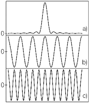
Figure 8: Power patterns for different antenna configurations. The horizontal axis in this figure is angle. Panel (a) shows that of a uniformly illuminated full aperture with a full width to half power (FWHP) of $k\,\lambda/D$, with $k\approx 1$ . In panel (b) we show the power pattern of a two element multiplying interferometer consisting of two antennas of diameter $d$ spaced by a distance $D$ where $d\ll D$. In panel (c) we show the power pattern of the interfermeter system described in (b) but now with a spacing $2D$.

If a uniform source is extended in angle by a positive and a negative fringe in Fig. 8 the response of the multiplied output is zero. For source structure smaller than a fringe, the response is not diminished. Thus by increasing $D$, finer and finer source structure is measured. Combining the outputs of independent data sets for spacings of $D$ and $2D$ shows that these select different structural components of the source. Finer source structure can be recorded if in addition, $D\,n$ antenna spacings are measured. Such a series measurements can be made by increasing the separation of two antennas whose outputs are coherently combined.

A general procedure, aperture synthesis, is now the standard method to obtain high quality, high angular resolution images. The first practical demonstration of aperture synthesis in radio astronomy was made by Ryle and his associates. Aperture synthesis allows us to reproduce the imaging properties of a large aperture by sampling the radiation field at individual positions within the area contained within the aperture. In analogy with the approach used by Michelson in the optical wavelength range, the advance in radio astronomy was to measure the mutual coherence function and to show that these results were sufficient to produce images. Using this approach, a remarkable improvement of the radio astronomical imaging was possible.

Electromagnetic waves induce the voltage $U_{1}$ at the output of antenna $A_{1}$

$$U_{1}\propto E{\rm\,e}^{\,{\rm\,i\,}\omega t}\,,$$ (82)

while at $A_{2}$ we obtain

$$U_{2}\propto E{\rm\,e}^{\,{\rm\,i\,}\omega\,(t-\tau)}\,,$$ (83)

where $E$ is the amplitude of the incoming plane wave, $\tau$ is the geometric delay caused by the relative orientation of the interferometer baseline $\vec{B}$ and the direction of the wave propagation. For simplicity, in (82) and (83) we have neglected receiver noise and instrumental phase. The outputs will be correlated. Today, all interferometers use direct correlation, since the goal is to measure the correlation accurately.

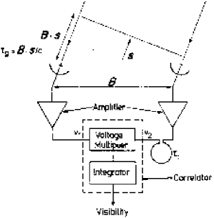
Figure 9: A schematic diagram of a two-element correlation interferometer. The antenna output voltages are $V_{1}$ and $V_{2}$; the instrumental delay is $\tau_{\rm i}$ and the geometric delay is $\tau_{\rm g}$ (from RW4 ).

In a correlation the signals are input to a multiplying device followed by an integrator. The output is proportional to

$$R(\tau)\propto\frac{E^{2}}{T}\int\limits_{0}^{T}{\rm\,e}^{\,{\rm\,i\,}\omega t}{\rm\,e}^{\,-{\rm\,i\,}\omega(t-\tau)}\,{\rm\,d}t\,.$$

If $T$ is a time much longer than the time of a single full oscillation, i.e., $T\gg 2\pi/\omega$ then the average over time $T$ will not differ much from the average over a single full period; that is

$$R(\tau) \propto \frac{\omega}{2\pi}E^{2}\int\limits_{0}^{2\pi/\omega}{\rm\,e}^{\,{\rm\,i\,}\omega\tau}\,{\rm\,d}t$$

$$\propto \frac{\omega}{2\pi}E^{2}{\rm\,e}^{\,{\rm\,i\,}\omega\tau}\int\limits_{0}^{2\pi/\omega}\,{\rm\,d}t\,,$$

resulting in

$$\framebox{$\displaystyle R(\tau)\propto{\textstyle\frac{1}{2}}E^{2}{\rm\,e}^{\,{\rm\,i\,}\omega\tau}$}\quad.$$ (84)

The output of the correlator $+$ integrator thus varies periodically with $\tau$, the delay time. If the orientation of interferometer baseline $\vec{B}$ and wave propagation direction $\vec{s}$ remain invariable, $\tau$ remains constant, so does $R(\tau)$. But since $\vec{s}$ is slowly changing due to the rotation of the earth, $\tau$ will vary, and we will measure interference fringes as a function of time.

In order to understand the response of interferometers in terms of measurable quantities, we consider a two-element system. The basic constituents are shown in Fig. 9. If the radio brightness distribution is given by $I_{\nu}(\vec{s})$, the power received per bandwidth ${\rm\,d}\nu$ from the source element ${\rm\,d}\Omega$ is $A(\vec{s})I_{\nu}(\vec{s}){\rm\,d}\Omega{\rm\,d}\nu$, where $A(\vec{s})$ is the effective collecting area in the direction $\vec{s}$; we will assume the same $A(\vec{s})$ for each of the antennas. The amplifiers are assumed to have constant gain and phase factors (neglected for simplicity).

The output of the correlator for radiation from the direction $\vec{s}$ (Fig. 9) is

$$r_{12}=A(\vec{s})\,I_{\nu}(\vec{s})\,{\rm\,e}^{{\rm\,i\,}\omega\tau}\,{\rm\,d}\Omega{\rm\,d}\nu$$ (85)

where $\tau$ is the difference between the geometrical and instrumental delays $\tau_{\rm g}$ and $\tau_{\rm i}$. If $\vec{B}$ is the baseline vector for the two antennas

$$\tau=\tau_{\rm g}-\tau_{\rm i}=\frac{1}{c}\,\vec{B}\cdot\vec{s}-\tau_{\rm i}$$ (86)

and the total response is obtained by integrating over the source $S$

$$\framebox{$\displaystyle R(\vec{B})=\parbox{22.76219pt}{$\vspace*{-2mm}{\displaystyle\int\!\!\int\atop{\!\!\!\!\!\scriptstyle\Omega}}$ }A(\vec{s})I_{\nu}(\vec{s})\exp\left[{\rm\,i\,}2\pi\nu\left(\frac{1}{c}\,\vec{B}\cdot\vec{s}-\tau_{\rm i}\right)\right]{\rm\,d}\Omega{\rm\,d}\nu$}\quad$$ (87)

This function $R(\vec{B})$, the Visibility Function is closely related to the mutual coherence function of the source, except for the power pattern $A(\vec{s})$ of the individual antennas. For parabolic antennas it is usually assumed that $A(\vec{s})=0$ outside the main beam area so that (87) is integrated only over this region. A one dimensional version of (87), with a baseline $B$, $\nu=\nu_{0}$ and $\tau_{i}=0$, is

$$R(B)=\int A(\theta)\,I_{\nu}(\theta)\exp\left[{\rm\,i\,}2\pi\nu_{0}\left(\frac{1}{c}\,B\cdot\theta\right)\right]{\rm\,d}\theta$$ (88)

Such a one dimensional relation is a very useful guide to understand interferometer responses.

7.1.1 Calibration

Two quantities that must be calibrated for continuum measurements are amplitude and phase. In addition, for spectral line measurements the instrument passband must also calibrated.

The amplitude scale is calibrated using methods that are similar to those used for single dish measurements. This consists of using the response of each antenna to determine the system noise of the receiver being used. In the centimeter range, the atmosphere plays a small role while in the millimeter and sub-mm wavelength ranges, the atmospheric effects must be accounted for. For phase measurements, a suitable point-like source with an accurately known position is required to determine the instrumental phase $2\pi\nu\tau_{i}$ in (87). For interferometers, the calibration sources are usually unresolved or point-like sources. Most often these are extragalactic time variable sources. To calibrate the response in units of flux density or brightness temperatures, these measurements must be referenced to a thermal calibrator.

The calibration of the instrument passband is carried out by an integration of an intense source to determine the channel-to-channel gains and offsets. The amplitude, phase and passband calibrations are carried out before the source measurements. The passband calibration is usually carried out once per observing session. The amplitude and phase calibrations are made more often. Their frequency depends on the stability of the electronics and weather. At millimeter wavelengths, the calibrations are usually made every few minutes, but may have to be made more often in worse weather or at shorter wavelengths. If weather demands that frequent measurements of calibrators are required, this is referred to as fast switching.

7.2 Responses of Interferometers

7.2.1 Finite Bandwidth

Eq. 87 can be used to estimate the effect of a finite bandwidth $\Delta\nu\,$. The geometric delay $\tau_{\rm g}=\frac{1}{c}\vec{B}\cdot\vec{s}\,$ is by definition independent of frequency, but the instrumental delay $\tau_{\rm i}\,$ may not be. Adjusting $\tau_{\rm i}\,$ the sum $\tau=\tau_{\rm g}-\tau_{\rm i}\,$ can be made equal to zero for the center of the band. Introducing the relative phase of a wave by

$$\varphi=\left[\frac{c\tau}{\lambda}\right]_{\rm fractional\;part}$$

we obtain

$$\varphi=\frac{1}{\lambda}\vec{B}\cdot\vec{s}+\varphi_{\rm i}\;,$$ (89)

where $\varphi_{\rm i}\,$ is the instrumental phase corresponding to the instrumental delay. This phase difference varies across the band of the interferometer $\Delta\nu\,$ by

$$\Delta\varphi=\frac{1}{\lambda}\vec{B}\cdot\vec{s}\,\frac{\Delta\nu}{\nu}.$$ (90)

The fringes will disappear when $\Delta\varphi\simeq 1\,$ radian. As can be seen the response is reduced if the frequency range, that is, the bandwidth, is large compared to the delay caused by the separation of the antennas. For large bandwidths, the loss of visibility can be minimized by adjusting the phase delay the time difference (see Fig. 9) is negligible. In effect, this is only possible if the exponential term in (87) is kept small. In practice, this is done by inserting a delay between the antennas so that $\frac{1}{c}\,\vec{B}\cdot\vec{s}$ equals $\tau_{\rm i}$. In the first interferometric systems this was done by switching lengths of cable into the system; currently this is accomplished by first digitizing the signal after conversion to an intermediate frequency, and then using digital shift registers. In analogy with the optical wavelength range, this adjustment of cable length is equivalent to centering the response on the central, or white light fringe in Young’s two-slit experiment.

The reduction of the response caused by finite bandwidth can be estimated by an integration of (87) over frequency. Taking $A(\vec{s})$ and $I_{\nu}(\vec{s})$ to be constants, and integrating over a range of frequencies $\Delta\nu=\nu_{1}-\nu_{2}$. Then the result is an additional factor, $\sin(\Delta\nu\tau)/\Delta\nu\tau\,$ in (87). This will reduce the interferometer response if $\Delta\varphi\sim 1$ . For typical bandwidths of 100 MHz, the offset from the zero delay must be $\ll 10^{-8}$ s. This adjustment of delays is referred to as fringe stopping. This causes the response of (87) to lose a component. To recover this input, an extra delay of a quarter wavelength relative to the input of the correlator is inserted, so that the sine and cosine response in (87) can be measured. In digital cross-correlators, (see Sect. 4.6), the sine and cosine components are obtained from the positive and negative delays. The component with even symmetry is the cosine component, while that with odd symmetry is the sine component.

7.2.2 Source Size and Minimum Spacing

Use 88 in the following. For an idealized source, of shape $I(\nu_{0})=I_{0}$ for $\theta\,<\,\theta_{0}$ and $I(\nu_{0})=0$ for $\theta\,>\,\theta_{0}$; we take the primary beamsize of each antenna to be much larger, and define the fringe width for a baseline $B$ $\theta_{b}$ to be $\frac{\lambda}{B}$, The result is

$$R(B)=A\,I_{0}\cdot\theta_{0}\,\exp\left[{\rm\,i\,}\pi\frac{\theta_{0}}{\theta_{b}}\right]\,\left[\frac{\sin{(\pi\theta_{0}/\theta_{b})}}{{(\pi\theta_{0}/\theta_{b})}}\right]$$ (91)

The first terms are normalization and phase factors. The important term, in the second set of brackets, is a $\sin{x}/x$ function. If $\theta_{0}>>\theta_{b}$, the interferometer response is reduced. This is sometimes refered to as the problem of “missing short spacings”.

7.2.3 Bandwidth and Beam Narrowing

In 7.2.1, we noted that on the white light fringe the compensation must reach a certain accuracy to prevent a reduction in the interferometer response. However for a finite primary antenna beamwidth, $A$, this cannot be the case over the entire beam. For two different wavelengths $\lambda_{l}$ and $\lambda_{s}$, there will be a phase difference

$$\Delta\phi=2\pi\,d\left[\frac{\sin{(\theta_{\rm offset})}}{\lambda_{s}}-\frac{\sin{(\theta_{\rm offset})}}{\lambda_{l}}\right]$$

converting the wavelengths to frequencies, and using $\sin{\theta}=\theta$, we have

$$\Delta\phi=2\pi\,\theta_{\rm offset}\,\frac{d}{c}\,\Delta\nu$$

With use of the relation $d=\frac{\lambda}{\theta_{b}}$, we have

$$\Delta\phi=2\pi\,\frac{\theta_{\rm offset}}{\theta_{b}}\,\frac{\Delta\nu}{\nu}$$ (92)

The effect in Eq. 92 is most important for continuum measurements made with large bandwidths. This effect can be reduced if the cross correlation is carried out using a series of contiguous IF sections. For each of these IF sections, an extra delay is introduced to center the response at the value which is appropriate for that wavelength before correlation.

7.3 Aperture Synthesis

Aperture Synthesis is a designation for methods used to derive the intensity distribution $I_{\nu}(\vec{s})$  of a part of the radio sky from the measured function $R(\vec{B})$. To accomplish this we must invert the integral equation (87). This involves Fourier transforms. For even simple images, a large number of computations are needed. Thus Aperture Synthesis and digital computing are intimately connected. In addition, a large number of approximations to be applied. We will outline the most important steps of this development without, however, claiming completeness.

For mm/sub-mm imaging, the relevant relation is:

$$\framebox{$\displaystyle I^{\prime}(x,y)=A(x,y)\,I(x,y)=\int\limits_{-\infty}^{\infty}V(u,v,0){\rm\,e}^{-{\rm\,i\,}2\pi(ux+vy)}{\rm\,d}u{\rm\,d}v$}\quad$$ (93)

where $I^{\prime}(x,y)$ is the intensity $I(x,y)$ modified by the primary beam shape $A(x,y)$. One can easily correct $I^{\prime}(x,y)$ by dividing by $A(x,y)$.

Important definitions are:

(1) Dynamic Range: The ratio of the maximum to the minimum intensity in an image. In images made with an interferometer array, it should be assumed tha the corrections for primary beam taper have been applied. If the minimum intensity is determined by the random noise in an image, the dynamic range is defined by the signal to noise ratio of the maximum feature in the image. The dynamic range is an indication of the ability to recognize low intensity features in the presence of intense features. If the minimum noise is determined by artefacts, i. e.noise in excess of the theoretical noise, the image can be improved by ^′image improvement techniques^′.

(2) Image Fidelity: Thisis defined by the agreement between the measured results and the actual (so-called ^′′true^′′) source structure. A quantitiave comparison would be

$$F=|(S-R)|/R$$

where $F$ is the fidelity, $R$ is the resulting image obtained from the measurement, and $S$ is the actual source structure.Of course one cannot have a priori knowledge of the correct source structure. In the case of simulations, $S$ is a source model, $R$ is the result of processing $S$ through $R$.

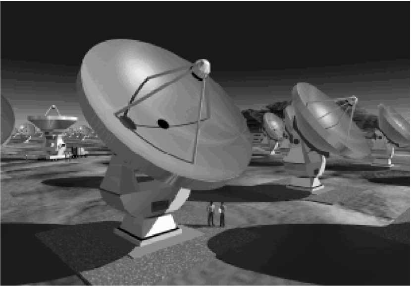
Figure 10: The most ambitious construction project in radio astronomy is the Atacama Large Millimeter Array (ALMA). ALMA will be built in north Chile on a 5 km high site. It will consist of at least fifty-four 12-m and twelve 7-m antennas, operating in 10 bands between wavelength 1cm and 0.3mm. The ALMA project is ambitious because of the superconducting receivers, the need for highly accurate antennas operating in the open, and the high altitude site. In addition, the data rates will be orders of magnitude higher than any existing astronomical facility. At the longest antenna spacing, and shortest wavelength, the angular resolution will be $\approx$5 milli arcseconds (courtesy European Southern Observatory).

7.3.1 Interferometric Observations

Usually measurements are carried out in 1 of 3 ways.

• In the first procedure, measurements of the source of interest and a calibrator are made. This is as in the case of single telescope position switching. Two significant differences with single dish measurements are that the interferometer measurement may have to extend over a wide range of hour angles to provide a better coverage of the $uv$ plane, and that instrumental phase must be determined also. One first measures a calibration source or reference source, which has a known position and size, to remove the effect of instrumental phases in the instrument and atmosphere and to calibrate the amplitudes of the sources in question. Sources and calibrators are usually observed alternately. The time variations caused by instrumental and weather effects must be slower than the time between measurements of source and calibrator. If, as is the case for mm/sub-mm wavelength measurements, weather is an important influence, one must switch frequently between target source and calibration source. In fast switching one might spend 10 seconds on a nearby calibrator, then a few minutes on-source. This method will reduce the amount of phase fluctuations, but also the amount time available for source measurements. For more rapid changes in the earth’s atmosphere, one can correct the phase using measurements of atmospheric water vapor, or changes in the system noise temperature of the individual receivers caused by atmospheric effects. The corrections for instrumental amplitudes and phases are assumed to be constant over the times when the source is observed. The ratio of amplitudes of source and calibrator are taken to be the normalized source amplitudes. Since the calibrators have known flux densities and positions, the flux densities and positions of the sources can be determined. The reference source should be as close to the on-source as possible, but must have a large enough intensity to guarantee a good signal-to-noise ratio after a short time. Frequently nearby calibrators are time variable over months, so a more distant calibrator with a known or fixed flux density is measured at the beginning or end of the session. This source is usually rather intense, so may also serve as a bandpass calibrator for spectral line measurements. The length of time spent on the off-source measurement is usually no more than few minutes.

• In the second procedure, the so-called snapshots, one makes a series of short observations (at different hour angles) of one source after another, and then repeats the measurements. For sensitivity reasons these are usually made in the radio continuum or intense maser lines. As in the first observing method, one intersperses measurements of a calibration source which has a known position and size to remove the effect of instrumental phases in the instrument and atmosphere and to calibrate the amplitudes of the sources in question. The images are affected by the shape of the synthesized beam of the interferometer system. If the size of the source to be imaged is comparable to the primary beam of the individual telescopes, the power pattern of the primary beams will have a large effect. This effect can be corrected easily.

• In the third procedure, one aims to produce a high-resolution image of a source where the goal is either high dynamic range or high sensitivity. The dynamic range is the ratio of the highest to the lowest brightness level of reliable detail in the image. This may depend on the signal-to-noise ratio for the data, but for centimeter aperture synthesis observations, spurious features in the image caused by the incomplete sampling of the $(u,v)$ plane are usually more important than the noise. Frequently one measures the source in a number of different interferometer configurations to better fill the $uv$ plane. These measurements are taken at different times and after calibration, the visibilities are entered into a common data set.

  An extension of this procedure may involve the measurement of adjacent regions of the sky. This is mosaicing. In a mosaic, the primary beams of the telescopes should overlap, ideally this would be at the half power point. In the simplest case, the images are formed separately and then combined to produce an image of the larger region.

  In order to eliminate the loss of source flux density due to missing short spacings, one must supplement the interferometer data with single dish measurements. The diameter of the single dish telescope should be larger than the shortest spacing between interferometer dishes. This single dish image must extend to the FWHP of the smallest of the interferometer antennas. When Fourier transformed and appropriately combined with the interferometer response, this data set has no missing flux density. Even in a data set containng single dish data, there are $``$missing spacings^′′. Improvements that can be applied to images produced from such data sets will be surveyed next.

7.3.2 Real Time Improvements of Visibility Functions

Ideally the relation between the measured $\widetilde{V_{ik}}$ visibility and the actual visibility $V_{ik}$ can be considered to be linear

$$\widetilde{V_{ik}}(t)=g_{i}(t)\,g^{*}_{k}(t)\,V_{ik}+\varepsilon_{ik}(t)\;.$$ (94)

Average values for the antenna gain factors $g_{k}$ and the noise term $\varepsilon_{ik}(t)$ are determined by measuring calibration sources as frequently as possible. Actual values for $g_{k}$ are then computed by linear interpolation. These methods make full use of the fact that the (complex) gain of the array is obtained by multiplication the gains of the individual antennas. If the array consists of $n$ such antennas, $n(n-1)/2$ visibilities can be measured simultaneously, but only $(n-1)$ independent gains $g_{k}$ are needed (for one antenna, one can arbitrarily set $g_{k}=1$ as a reference). In an array with many antennas, the number of antenna pairs greatly exceeds the number of antennas. For phase, one must determine $n$ phases.

Often these conditions can be introduced into the solution in the form of closure errors. Introducing the phases $\varphi,\theta$ and $\psi$ by
$$\begin{array}[]{rcl}\widetilde{V_{ik}}&=&|\widetilde{V_{ik}}|\,\exp\left\{{\rm\,i\,}\varphi_{ik}\right\}\,,\\ G_{ik}&=&|g_{i}|\,|g_{k}|\,\exp\left\{{\rm\,i\,}\theta_{i}\right\}\exp\left\{-{\rm\,i\,}\theta_{k}\right\}\,,\\ V_{ik}&=&|V_{ik}|\,\exp\left\{{\rm\,i\,}\psi_{ik}\right\}\,.\\ \end{array}$$ (95)
From (94) the visibility phase $\psi_{ik}$ on the baseline $ik$ will be related to the observed phase $\varphi_{ik}$ by

$$\varphi_{ik}=\psi_{ik}+\theta_{i}-\theta_{k}+\varepsilon_{ik}\,,$$ (96)

where $\varepsilon_{ik}$ is the phase noise. Then the closure phase $\Psi_{ikl}$ around a closed triangle of baseline $ik,kl,li$,

$$\Psi_{ikl}=\varphi_{ik}+\varphi_{kl}+\varphi_{li}=\psi_{ik}+\psi_{kl}+\psi_{li}+\varepsilon_{ik}+\varepsilon_{kl}+\varepsilon_{li}\,,$$ (97)

will be independent of the phase shifts $\theta$ introduced by the individual antennas and the time variations. With this procedure, on can minimize phase errors.

Closure amplitudes can also be formed. If four or more antennas are used simultaneously, then ratios, the so-called closure amplitudes, can be formed. These are independent of the antenna gain factors:

$$A_{klmn}=\frac{|V_{kl}||V_{mn}|}{|V_{km}||V_{ln}|}=\frac{|\Gamma_{kl}||\Gamma_{mn}|}{|\Gamma_{km}||\Gamma_{ln}|}\;.$$ (98)

Both phase and closure amplitudes can be used to improve the quality of the complex visibility function.

If each antenna introduces an unknown complex gain factor $g$ with amplitude and phase, the total number of unknown factors in the array can be reduced significantly by measuring closure phases and amplitudes. If four antennas are available, 50 % of the phase information and 33 % of the amplitude information can thus be recovered; in a 10 antenna configuration, these ratios are 80 % and 78 % respectively.

7.3.3 Multi-Antenna Array Calibrations

For two antenna interferometers, phase calibration can only be made pair-wise. This is referred to as ^′baseline based^′ solutions for the calibration. For a multi-antenna system, there are other and better methods. One can use sets of three antennas to determine the best phase solutions and then combine these to optimize the solution for each antenna. For amplitudes, one can combine sets of four antennas to determine the best amplitude solutions and then optimize this solution to determine the best solution. This process leads to ^′antenna based^′ solutions are used. Antenna based calibrations are used in most cases. These are determined by applying phase and amplitude closure for subsets of antennas and then making the best fit for a given antenna. It is important to note that because of (50) the output of an antenna can be amplified without seriously degrading the signal-to-noise ratio. For this reason, cross-correlations between a large number of antennas is possible in the radio and mm/sub-mm ranges. This is not the case in the optical or near-IR ranges.

7.4 Interferometer Sensitivity

The random noise limit to an interferometer system is calculated following the method used for a single telescopeRW4 . The RMS fluctuations in antenna temperature are

$$\Delta T_{\rm A}=\frac{M\,T_{\rm sys}}{\sqrt{t\,\Delta\nu}}\,,$$ (99)

where $M$ is a factor of order unity used to account for extra noise from analog to digital conversions, digital clipping etc. If we next apply the definition of flux density, ${S_{\nu}}$ in terms of antenna temperature for a two-element system, we find:

$$\Delta S_{\nu}=2\,k\,\frac{T_{\rm sys}{\rm\,e}^{\tau}}{A_{\rm e}\sqrt{2t\,\Delta\nu}}\,,$$ (100)

where $\tau$ is the atmospheric optical depth and $A_{\rm e}$ is the effective collecting area of a single telescope of diameter $D$. There is additional in this expression since a multiplying interferometer does not process all of the information (i. e. the total power) that the antennas receive. In this case, there is an additional factor of $\sqrt{2}$ compared to the noise in a single dish with an equivalent collecting area since there is information not collected by a multiplying interferometer. We denote the system noise corrected for atmospheric absorption by $T_{\rm sys}^{\prime}=T_{\rm sys}\exp{\tau}$, in order to simplify the following equations. For an array of $n$ identical telescopes, there are $N=n(n-1)/2$ simultaneous pair-wise correlations. Then the RMS variation in flux density is

$$\Delta S_{\nu}=\frac{2\,M\,k\,T_{\rm sys}^{\prime}}{A_{\rm e}\sqrt{2\,N\,t\,\Delta\nu}}\,.$$ (101)

This relation can be recast in the form of brightness temperature fluctuations using the Rayleigh-Jeans relation;

$$S=2\,k\,\frac{T_{\rm b}\,\Omega_{b}}{\lambda^{2}}\,.$$ (102)

Then the RMS brightness temperature, due to random noise, in aperture synthesis images is

$$\Delta T_{\rm b}=\frac{2\,M\,k\,\lambda^{2}\,T_{\rm sys}^{\prime}}{A_{\rm e}\Omega_{\rm b}\sqrt{2\,N\,t\,\Delta\nu}}\,.$$ (103)

For a Gaussian beam, $\Omega_{\rm mb}=1.133\,\theta^{2}$, so we can relate the RMS temperature fluctuations to observed properties of a synthesis image. The ALMA sensitivity calculator is to be found at

http://www.eso.org/sci/facilities/ALMA/observing/tools

At shorter wavelengths, the RMS temperature fluctuations are lower. Thus, for the same collecting area and system noise, if weather changes are unimportant, a millimeter image should be more sensitive than an image made at centimeter wavelengths. If the effective collecting area remains the same and for a larger main beam solid angle, temperature fluctuations will decrease. For this reason, smoothing an image will result in a lower RMS noise in an image. However, if smoothing is too extreme, this process effectively leads to a decrease in collecting area; then there will be no further improvement in sensitivity.

The temperature sensitivity (in Kelvins) for higher angular resolution is worse than for a single telescope with an equal collecting area. From the Rayleigh-Jeans relation, the sensitivity in Jansky (Jy) is fixed by the antenna collecting area and the receiver noise, so only the wavelength and the angular resolution can be varied. Thus, the increase in angular resolution is made at the expense of temperature sensitivity. All other effects being equal, at shorter wavelengths one gains in temperature sensitivity

Compared to single dishes, interferometers have the great advantage that uncertainties such as pointing and beam size depend fundamentally on timing. Such timing uncertainties can be made very small compared to all other uncertainties. In contrast, the single dish measurements are critically dependent on mechanical deformations of the telescope. In summary, the single dish results are easier to obtain, but source positions and sizes on arc second scales are difficult to estimate. The interferometer system has a much greater degree of complexity, but allows one to measure such fine details. The single dish system responds to the source irrespective of the relation of source to beam size; the correlation interferometer will not record source structures larger than a few fringes.

Aperture synthesis is based on sampling the visibility function $V(u,v)$ with separate antennas to provide samples in the $(u,v)$ plane. Many configurations are possible, but the goal is the densest possible coverage of the $(u,v)$ plane. If one calculates the RMS noise in a synthesis image obtained by simply Fourier transforming the $(u,v)$ data, one usually finds a noise level many times higher than that given by (103) or (101). There are various reasons for this. One cause is phase fluctuations due to atmospheric or instrumental influences such as LO instabilities. Another cause is due to incomplete sampling of the $(u,v)$ plane. This gives rise to instrumental features, such as stripe-like features in the final images. Yet another systematic effect is the presence of grating rings around more intense sources; these are analogous to high side lobes in single dish diffraction patterns. Over the past 20 years, it has been found that these effects can be substantially reduced by software techniques such as CLEAN and Maximum Entropy.

7.4.1 Post Real Time Improvements of Visibility Functions

Before applying specialized techniques, the data must be organized in a useful way without lowering the signal-to-noise ratios. To speed up computations for inverting (93) one uses the Cooley-Tukey fast Fourier transform algorithm. In order to use the FFT in its simplest version, the visibility function must be placed on a regular grid with sizes that are powers of two of the sampling interval. Since the observed data seldom lie on such regular grids, an interpolation scheme must be used. If the measured points are randomly distributed, this interpolation is best carried out using a convolution procedure.

If some of the spatial frequencies present in the intensity distribution are not present in the $(u,v)$ plane data, then changing the amplitude or phase of the corresponding visibilities will not have any effect on the reconstructed intensity distribution – these have been eliminated. The extent of this effect is shown by the ^′′dirty beam^′′.

Expressed mathematically, if $Z$ is an intensity distribution containing only the unmeasured spatial frequencies, and $P_{\rm D}$ is the dirty beam, then

$P_{\rm D}\otimes Z=0$.

Hence, if $I$ is a solution of the convolution equation (105) then so is $I+\alpha Z$ where $\alpha$ is any number. This shows that there is no unique solution to the problem.

The solution with visibilities $V=0$ for the unsampled spatial frequencies is usually called the principal solution, and it differs from the true intensity distribution by some unknown invisible or ghost distribution. It is the aim of image reconstruction to obtain reasonable approximations to these ghosts by using additional knowledge or plausible extrapolations, but there is no direct way to select the ^′′best^′′ or ^′′correct^′′ image from all possible images. The familiar linear deconvolution algorithms are not adequate and nonlinear techniques must be used.

The result obtained from the gridded $uv$ data can be Fourier transformed to obtain an image with a resolution corresponding to the size of the array. However, this may still contain artifacts caused by the details of the observing procedure, especially the limited coverage of the ($uv$) plane. Therefore the dynamic range of such so-called dirty maps is rather small. This can be improved by further data analysis, as will be described next.

If the calibrated visibility function $V(u,v)$ is known for the full $(u,v)$ plane both in amplitude and in phase, this can be used to determine the (modified) intensity distribution $I^{\prime}(x,y)$ by performing the Fourier transformation (93). However, in a realistic situation $V(u,v)$ is only sampled at discrete points within a radius $\cong u_{\rm max}$ along elliptical tracks, and in some regions of the $(u,v)$ plane, $V(u,v)$ is not measured at all.

We can weight the visibilities by a grading function, $g$. Then for a discrete number of visibilities, we have a version of (93) involving a summation, not an integral, to obtain an image via a discrete Fourier transform (DFT):

$$I_{\rm D}(x,y)=\sum_{k}g(u_{k},v_{k})V(u_{k},v_{k}){\rm\,e}^{-{\rm\,i\,}2\pi(u_{k}x+v_{k}y)}\,,$$ (104)

where $g(u,v)$ is a weighting function called the grading or apodisation. To a large extent $g(u,v)$ is arbitrary and can be used to change the effective beam shape and side lobe level. There are two widely used weighting functions: uniform and natural. Uniform weighting uses $g(u_{k},v_{k})=1$, while Natural weighting uses $g(u_{k},g_{k})=1/N_{\rm s}(k)$, where $N_{\rm s}(k)$ is the number of data points within a symmetric region of the $(u,v)$ plane. In a simple case $N_{\rm s}(k)$ would be a square centered on point $k$. Data which are naturally weighted result in lower angular resolution but give a better signal-to-noise ratio than uniform weighting. But these are only extreme cases. One can choose intermediate weighting schemes. These are often referred to as robust weighting (in the nomenclature of the AIPS data reduction package). Often the reconstructed image $I_{\rm D}$ may not be a particularly good representation of $I^{\prime}$, but these are related. In another form, (104) is

$$I_{\rm D}(x,y)=P_{\rm D}(x,y)\otimes I^{\prime}(x,y)\,,$$ (105)

where

$$P_{\rm D}=\sum_{k}g(u_{k},v_{k}){\rm\,e}^{-{\rm\,i\,}2\pi(u_{k}x+v_{k}y)}$$ (106)

is the response to a point source. This is the point spread function PSF for the dirty beam. Thus the dirty beam can be understood as a transfer function that distorts the image. (The dirty beam, $P_{\rm D}$, is produced by the Fourier transform of a point source in the regions sampled; this is the response of the interferometer system to a point source). That is, the dirty map $I_{\rm D}(x,y)$ contains only those spatial frequencies $(u_{k},v_{k})$ where the visibility function has been measured. The sum in (106) extends over the same positions $(u_{k},v_{k})$ as in (104), and the side lobe structure of the beam depends on the distribution of these points.

7.5 Advanced Image Improvement Methods

Digital computing is clearly a crucial part of synthesis array data processing. A large part of the advances in radio synthesis imaging during the last 15–20 years relies on the progress made in the field of image restoration. In the following we present a few schemes that are applied to improve radio images. However this is by no means an exhaustive collection.

7.5.1 Self-Calibration

Amplitude and phase errors scatter power across the image, giving the appearance of enhanced noise. Quite often this problem can be alleviated to an impressive extent by the method of self-calibration. This process can be applied if there is a sufficiently intense source in the field contained within the primary beam of the interferometer system. Basically, self-calibration is the equivalent of focusing on the source, analogous to using the focus of a camera to sharpen up an object in the field of view. One can restrict the self-calibration to an improvement of phase alone or to both phase and amplitude. However, self-calibration is carried in the $(u,v)$ plane. If properly used, this method leads to a great improvement in interferometer images of compact intense sources such as those of masering spectral lines. If this method is used on objects with low signal-to-noise ratios, this method may give very wrong results by concentrating random noise into one part of the interferometer image (see CORNWEL ).

In measurements of weak spectral lines, the self-calibration is carried out with a continuum source in the field. The corrections are then applied to the spectral line data. In the case of intense lines, one of the frequency channels containing the emission is used. If self-calibration is applied, the source position information is usually lost.

7.5.2 Applying CLEAN to the Dirty Map

CLEANing is the most commonly used technique to improve single radio interferometer images(HOGBOM ). The dirty map is a representation of the principal solution, but with shortcomings. In addition to its inherent low dynamic range, the dirty map often contains features such as negative intensity artifacts. These cannot be real. Another unsatisfactory aspect is that the principal solution is quite often rather unstable, in that it can change drastically when more visibility data are added. Instead of a principle solution that assumes $V=0$ for all unmeasured visibilities, values for $V$ should be adopted at these positions in the $(u,v)$ plane. These are obtained from some plausible model for the intensity distribution.

The CLEAN method approximates the actual but unknown intensity distribution $I(x,y)$ by the superposition of a finite number of point sources with positive intensity $A_{i}$ placed at positions $(x_{i},y_{i})$. It is the aim of CLEAN to determine the $A_{i}(x_{i},y_{i})$ such that

$$I^{\prime\prime}(x,y)=\sum_{i}A_{i}\,P_{\rm D}(x-x_{i},y-y_{i})+I_{\varepsilon}(x,y)\,$$ (107)

where $I^{\prime\prime}$ is the dirty map obtained from the inversion of the visibility function and $P_{\rm D}$ is the dirty beam (106). $I_{\varepsilon}(x,y)$ is the residual brightness distribution after decomposition. Approximation (107) is deemed successful if $I_{\varepsilon}$ is of the order of the noise in the measured intensities. This decomposition cannot be done analytically, rather an iterative technique has to be used.

The CLEAN algorithm is most commonly applied in the image plane. This is an iterative method which functions in the following fashion: First find the peak intensity of the dirty image, then subtract a fraction $\gamma$ with the shape of the dirty beam from the image. Then repeat this $n$ times. This loop gain $0<\gamma<1$ helps the iteration converge, and it is usually continued until the intensities of the remaining peaks are below some limit. Usually the resulting point source model is convolved with a clean beam of Gaussian shape with a FWHP similar to that of the dirty beam. Whether this algorithm produces a realistic image, and how trustworthy the resulting point source model really is, are unanswered questions.

7.5.3 Maximum Entropy Deconvolution Method (MEM)

The Maximun Entropy Deconvolution Method (MEM) is commonly used to produce a single optimal image from a set of separate but contiguous images GULL . The problem of how to select the $``$best^′′ image from many possible images which all agree with the measured visibilities is solved by MEM. Using MEM, those values of the interpolated visibilities are selected, so that the resulting image is consistent with all previous relevant data. In addition, the MEM image has maximum smoothness. This is obtained by maximizing the entropy of the image. One possible definition of entropy is given by

$${\cal H}=-\sum_{i}I_{i}\left[\ln\bigg{(}\frac{I_{i}}{M_{i}}\bigg{)}-1\right]\,,$$ (108)

where $I_{i}$ is the deconvolved intensity and $M_{i}$ is a reference image incorporating all $``$a priori^′′ knowledge. In the simplest case $M_{i}$ is the empty field $M_{i}={\rm const}>0$, or perhaps a lower angular resolution image.

Additional constraints might require that all measured visibilities should be reproduced exactly, but in the presence of noise such constraints are often incompatible with $I_{i}>0$ everywhere. Therefore the MEM image is usually constrained to fit the data such that

$$\chi^{2}=\sum\frac{|V_{i}-V_{i}^{\prime}|^{2}}{\sigma_{i}^{2}}$$ (109)

has the expected value, where $V_{i}$ is the measured visibility, $V_{i}^{\prime}$ is a visibility corresponding to the MEM image and $\sigma_{i}$ is the error of the measurement.

8 Continuum Emission from mm/sub-mm Sources

In the early days of mm/sub-mm wavelength astronomy receiver sensitivities restricted measurements to a few continuum sources. This has improved dramatically with the use of semiconductor bolometers pioneered by F. J. Low. Subsequently spectral lines of molecules such as CO, HCN and CS were found. These were rather intense, and this led to a blossoming of the field. Subsequently, spectral lines of neutral carbon and a line of ionized carbon were detected. We sketch continuum radiation mechanisms and then spectral line mechanisms that are specific to the mm/sub-mm wavelength range.

Radio sources can thus be classified into two categories: those which radiate by thermal mechanisms and the others, which radiate by nonthermal processes. In practice, non-thermal radiation can be explained by the synchrotron process. This is caused by relativistic electrons spiraling in a magnetic field (see SCHEUER for a delightful and instructive account). For optically thin synchrotron radiation, most sources have a flux density that varies as

$$\framebox{$\displaystyle S_{\nu}=S_{0}\,\left(\frac{\nu}{\nu_{0}}\right)^{-\alpha}$}$$ (110)

where $\alpha$ has a positive value. Synchrotron radiation often shows linear polarization, and in rare cases, shows circular polarization. The most prominent example of a synchrotron source with $\alpha=0$, i. e. a flat spectrum is Sgr A^∗. This source, at 8.5 kpc from the Sun, is considered to be the closest supermassive Black Hole. The variation of flux density with frequency may be an indication that the synchrotron emission is optically thick, and/or has a non-standard geometry (see, e. g. MARRONE ). Interferometry at 1.3 mm of Sgr A^∗ with baselines of up to a few 10³ km is ongoing. The imaging of Sgr A^∗ with astronomical unit linear resolution is of high interest. Measurements of synchrotron emission give only a very limited set of source parameters. When combined with other data, synchrotron measurements can be used to obtain source parameters (see RW5 ).

The most famous example of black body radiation is the 2.73 K cosmic microwave background, CMB. This source of radiation is fit by a Planck curve to better than 0.1 %. The difficulty in detecting it was not due to weak signals, but rather due to the fact that the radiation is present in all directions, so that scanning a telescope over the sky and taking differences will not lead to a detection. The actual discovery was gotten from measurements of the noise temperature from the sky, the receiver and the ground, compared to the temperature of a helium cooled load using Dicke switching. Studies of the CMB are conducted from satellites and balloons; these are directed at determinations of the polarization and deviations from the Black Body spectrum.

As an example of thermal radiation, we consider planets. These are black bodies with spectra that are an almost exact representation of the Rayleigh-Jeans law for various temperatures. For H ii regions such as Orion A the spectrum is not a simple black body, but explanation is fairly straightforward. If we consider the solution of the equation of radiation transfer (14) for an isothermal object without a background source

$$I_{\nu}=B_{\nu}(T)\,(1-{\rm\,e}^{-\tau_{\nu}})\,,$$

we find that $I_{\nu}<B_{\nu}$ if $\tau_{\nu}<1$; the frequency variation of $I_{\nu}$ depends on $\tau_{\nu}$ ALTENHOFF :

$$\framebox{$\displaystyle\tau_{\nu}=8.235\times 10^{-2}\left(\frac{T_{\rm e}}{\rm K}\right)^{-1.35}\left(\frac{\nu}{\rm GHz}\right)^{-2.1}\left(\frac{\rm EM}{\rm pc\,cm^{-6}}\right)\,a(\nu,T)$}$$ (111)

can be derived. The correction $a(\nu,T)$ is usually $\cong 1$. The term $EM$ is

$$EM=\int N_{e}^{2}{\rm\,d}l$$

with units cm^-6pc. This is a complex relation and was derived only after plowing through lots and lots of math. $N_{e}$ cannot be directly obtained from $EM$ because of clumping.

Figure 11: The spectrum of the star burst galaxy M82. The flux density scale must be multiplied by $10^{3}$. This galaxy is rather close to the Sun, but has a star formation rate that is much higher than for the Milky Way. The large featureless maximum is caused by dust radiation. On top of this are various molecular and atomic lines. The different curves represent M82 for the labelled redshifts. Although the emission decreases inversely with the square of the distance, this is compensated by the shift of dust radiation to lower frequencies. These effects allow one to detect an oject such as M82 to redshift $z=12$ with the Atacama Large Millimeter Array (ALMA). The ALMA receiver bands are indicated by numbers in the upper left side of this figure (P. Cox unpublished).

It appears that cold dust, with temperatures 10 K to 30 K, makes up much of the mass of dust and by implication traces cold interstellar gas, given a dust-to-gas ratio. Since the average size is thought to be $\sim$0.3$\mu$m, the wavelength of the radiation is much longer than the size of the emitter. For this reason, the efficiency of sub-mm radiation is rather low. Dust grains show linear polarization, which leads to the conclusion that grains are elongated and aligned by magnetic fields. The direction but not the strength of the magnetic field can be determined from dust polarization. The fractional polarization is rather small, so requires high sensitivity and care to keep instrumental effects smallENDRIK .

If we use the exact relation, we have

$$T_{\rm b}(\nu)=T_{0}\!\left(\frac{1}{{\rm exp}\{T_{0}/T_{\rm dust}\}-1}-\frac{1}{{\rm exp}\{T_{0}/2.7\}-1}\right)\!(1-{\rm\,e}^{-\tau_{\rm dust}})\,,$$ (112)

where $T_{0}=h\nu/k$. This is completely general; if we neglect the 2.7 K background,

$$T_{\rm dust}=T_{0}\left(\frac{1}{{\rm exp}\{T_{0}/T_{\rm dust}\}-1}\right)(1-{\rm\,e}^{-\tau_{\rm dust}})\,.$$ (113)

If $T_{\rm dust}\gg T_{0}$, we can simplify this expression, but the most important step is in making a quantitative connection between $\tau_{\rm dust}$ and $N_{\rm H_{2}}$. The relation between $\tau_{\rm dust}$ and the gas column density must be determined empirically. Unlike the planets, which have measured sizes, the radiation from dust grains depends on the surface area of the grains, which cannot be determined directly. If a relation between dust mass and $\tau$ can be determined, it is simple to convert to the total mass, since dust is generally accepted to be between 1/100 and 1/150 th of the total mass. All astronomical determinations are based on HILDEBRAND . One typical parameterized version is given by MEZGER : $\lambda>100\,{\rm\mbox{\greeksym{m}}m}$:

$$\tau_{\rm dust}=7\times 10^{-21}\,\frac{Z}{Z_{\odot}}\,b\,N_{\rm H}\,\lambda^{-2}$$ (114)

where $\lambda$ is the wavelength in mm, $N_{\rm H}$ is in units cm^-2, $Z$ is the metalicity as a ratio of that of the sun $Z_{\odot}$. The parameter $b$ is an adjustable factor used to take into account changes in grain sizes. Currently, it is believed that $b=1.9$ is appropriate for moderate density gas and $b=3.4$ for dense gas (but this is not certain). At long millimeter wavelengths, a number of observations have shown that the optical depth of such radiation is small. Then the observed temperature is

$$T=T_{\rm dust}\,\tau_{\rm dust}\,,$$ (115)

where the quantities on the right side are the dust temperature and optical depth. Then the flux density is

$$S=\frac{2\,k\,T}{\lambda^{2}}=2\,k\,T_{\rm dust}\lambda^{-2}\,\tau_{\rm dust}\Delta\Omega\,.$$ (116)

If the dust radiation is expressed in Jy, the source in FWHP sizes, $\theta$ in arc seconds, and the wavelength, $\lambda$ in mm, one has for the column density of hydrogen in all forms, $N_{\rm H}$, in the Rayleigh-Jeans approximation, the following relation:

If the dust radiation is expressed in mJy, the source FWHP size, $\theta$, in arc seconds, and the wavelength, $\lambda$ in mm, the column density of hydrogen in all forms, $N_{\rm H}$, in the Rayleigh-Jeans approximation, is:

$$N_{\rm H}=1.93\times 10^{24}\,\frac{S_{\nu}}{\theta^{2}}\,\frac{\lambda^{4}}{Z/Z_{\odot}\,b\,T_{\rm dust}}\,.$$ (117)

In the cm and mm wavelength range, the dust optical depth is small and increases as $\lambda^{-\beta}$ with $\beta$ values between 1 and 2; then flux density increases as $\lambda^{-3}$ to $\lambda^{-4}$.

Observationally, it has been determined that, in most cases, the dust optical depth increases with $\lambda^{-2}$; then flux density increases as $\lambda^{-4}$. Thus, dust emission will become more important at millimeter wavelengths and in the infrared. It might appear that Eq. 111 is more accurate than Eq.  117, because of the vast amount of math. However for a determination of $N_{e}$, source clumping introduces uncertainties.

9 Spectral Line Basics

In local thermodynamic equilibrium (LTE) the intensities of emitted and absorbed radiation are not independent but are related by Kirchhoff’s law (9). This applies to both continuous radiation and line radiation. The Einstein coefficients give a convenient means to describe the interaction of radiation with matter by the emission and absorption of photonsRYBICKI .These are:

[width=4.8cm,height=2.4cm]kap11f1.eps

Figure 12: Transitions between the states 1 and 2 and the Einstein probabilities

$$\framebox{$\displaystyle g_{1}\,B_{12}=g_{2}\,B_{21}$}$$ (118)

and

$$\framebox{$\displaystyle A_{21}=\frac{8\pi h\nu_{0}^{3}}{c^{3}}\,B_{21}$}\quad$$ (119)

9.1 Radiative Transfer with Einstein Coefficients

When the radiative transfer was considered in Sect. 2.1, the material properties were expressed as the emission coefficient $\varepsilon_{\nu}$ and the absorption coefficient $\kappa_{\nu}$. Both $\varepsilon_{\nu}$ and $\kappa_{\nu}$ are macroscopic parameters; for a physical theory these must to be related to atomic properties of the matter in the cavity. If line radiation is considered, the Einstein coefficients are very useful because these can be linked directly to the properties of the transition responsible for the spectral line. For radiative transfer $\varepsilon_{\nu}$ and $\kappa_{\nu}$ are needed, so we must investigate the relation between $\kappa_{\nu}$ and $A_{ik}$ and $B_{ik}$. This is best done by considering the possible change of intensity $I_{\nu}$ passing through a slab of material with thickness ${\rm\,d}s$ as in Sect. 2.1. Now we will use $A_{ik}$ and $B_{ik}$.

According to Einstein there are three different processes contributing to the intensity $I_{\nu}$. Each system making a transition from $E_{2}$ to $E_{1}$ contributes the energy $h\nu_{0}$ distributed over the full solid angle $4\pi$. Then the total amount of energy emitted spontaneously is

$${\rm\,d}E_{\rm e}(\nu)=h\nu_{0}\,N_{2}\,A_{21}\,\varphi_{\rm e}(\nu){\rm\,d}V\frac{{\rm\,d}\Omega}{4\pi}{\rm\,d}\nu{\rm\,d}t\,.$$ (120)

For the total energy absorbed we similarly obtain

$${\rm\,d}E_{\rm a}(\nu)=h\nu_{0}\,N_{1}\,B_{12}\,\frac{4\pi}{c}\,I_{\nu}\,\varphi_{\rm a}(\nu){\rm\,d}V\frac{{\rm\,d}\Omega}{4\pi}{\rm\,d}\nu{\rm\,d}t$$ (121)

and for the stimulated emission

$${\rm\,d}E_{\rm s}(\nu)=h\nu_{0}\,N_{2}\,B_{21}\,\frac{4\pi}{c}\,I_{\nu}\,\varphi_{\rm e}(\nu){\rm\,d}V\frac{{\rm\,d}\Omega}{4\pi}{\rm\,d}\nu{\rm\,d}t\,.$$ (122)

The line profiles $\varphi_{\rm a}(\nu)$ and $\varphi_{\rm e}(\nu)$ for absorbed and emitted radiation could be different, but in astrophysics it is usually permissible to put $\varphi_{\rm a}(\nu)=\varphi_{\rm e}(\nu)=\varphi(\nu)$. For the volume element we put ${\rm\,d}V={\rm\,d}\sigma{\rm\,d}s$, where ${\rm\,d}\sigma$ is the unit area perpendicular to the beam direction. For a stationary situation, we find

$${\rm\,d}E_{\rm e}(\nu)+{\rm\,d}E_{\rm s}(\nu)-{\rm\,d}E_{\rm a}(\nu)={\rm\,d}I_{\nu}{\rm\,d}\Omega{\rm\,d}\sigma{\rm\,d}\nu{\rm\,d}t$$

$$=\frac{h\nu_{0}}{4\pi}\left[N_{2}\,A_{21}+N_{2}\,B_{21}\,\frac{4\pi}{c}\,I_{\nu}-N_{1}\,B_{12}\,\frac{4\pi}{c}\,I_{\nu}\right]\varphi(\nu){\rm\,d}\Omega{\rm\,d}\sigma{\rm\,d}s{\rm\,d}\nu{\rm\,d}t\,.$$

The resulting equation of transfer with Einstein coefficients is

$$\framebox{$\displaystyle\frac{{\rm\,d}I_{\nu}}{{\rm\,d}s}=-\frac{h\nu_{0}}{c}\left(N_{1}\,B_{12}-N_{2}\,B_{21}\right)I_{\nu}\,\varphi(\nu)+\frac{h\nu_{0}}{4\pi}N_{2}\,A_{21}\,\varphi(\nu)$}\quad.$$ (123)

Comparing this with (8) we obtain agreement by putting

$$\framebox{$\displaystyle\kappa_{\nu}=\frac{h\nu_{0}}{c}\,N_{1}\,B_{12}\left(1-\frac{g_{1}N_{2}}{g_{2}N_{1}}\right)\varphi(\nu)$}$$ (124)

and

$$\framebox{$\displaystyle\varepsilon_{\nu}=\frac{h\nu_{0}}{4\pi}\,N_{2}\,A_{21}\,\varphi(\nu)$}\quad,$$ (125)

The factor in brackets in (124) is the correction for stimulated emission. In radio astronomy, where the stimulated emission almost completely cancels the effect of the true absorption, this is important. How this comes about is best seen if we investigate what becomes of (123–125) if LTE is assumed.

From (124) and (125) we find that

$$\frac{\varepsilon_{\nu}}{\kappa_{\nu}}=\frac{2h\nu^{3}}{c^{2}}\left(\frac{g_{2}N_{1}}{g_{1}N_{2}}-1\right)^{-1}\,.$$

But for LTE, according to (9), this should be equal to the Planck function, resulting in

$$\framebox{$\displaystyle\frac{N_{2}}{N_{1}}=\frac{g_{2}}{g_{1}}\exp\bigg{(}-\frac{h\nu_{0}}{k\,T}\bigg{)}$}\quad.$$ (126)

In LTE, the energy levels are populated according to the same Boltzmann distribution for the temperature $T$ that applied to full TE. Then the absorption coefficient becomes

$$\framebox{$\displaystyle\kappa_{\nu}=\frac{c^{2}}{8\pi}\frac{1}{\nu_{0}^{2}}\frac{g_{2}}{g_{1}}\,N_{1}\,A_{21}\left[1-\exp\left(-\frac{h\nu_{0}}{k\,T}\right)\right]\varphi(\nu)$}\quad,$$ (127)

where we have replaced the $B$ coefficient by the $A$ coefficient, using

$$B_{12}=\frac{g_{2}}{g_{1}}\,A_{21}\,\frac{c^{3}}{8\pi h\nu^{3}}\,.$$

9.2 Dipole Transition Probabilities

The simplest sources for electromagnetic radiation are oscillating dipoles. Radiating electric dipoles have already been treated classically, but it should also be possible to express these results in terms of the Einstein coefficients. There are two types of dipoles that can be treated by quite similar means: the electric and the magnetic dipole.

Electric Dipole. Consider an oscillating electric dipole

$$d(t)=e\,x(t)=e\,x_{0}\cos\omega t\,.$$ (128)

According to electromagnetic theory, this will radiate. The power emitted into a full $4\pi$ steradian is,

$$P(t)=\frac{2}{3}\frac{e^{2}\dot{v}(t)^{2}}{c^{3}}\,.$$ (129)

Expressing $x=d/e$ and $\dot{v}=\ddot{x}$, we obtain an average power, emitted over one period of oscillation of

$$\langle P\rangle=\frac{64\pi^{4}}{3\,c^{3}}\,\nu_{mn}^{4}\left(\frac{e\,x_{0}}{2}\right)^{2}\,.$$ (130)

This mean emitted power can also be expressed in terms of the Einstein $A$ coefficient:

$$\langle P\rangle=h\,\nu_{mn}\,A_{mn}\,.$$ (131)

Equating (130) and (131) we obtain

$$\framebox{$\displaystyle A_{mn}=\frac{64\pi^{4}}{3\,h\,c^{3}}\,\nu_{mn}^{3}\,|\mu_{mn}|^{2}$}\quad,$$ (132)

This was also cited in Section 2.3.1. where

$$\mu_{mn}=\frac{e\,x_{0}}{2}$$ (133)

is the mean electric dipole moment of the oscillator for this transition.

Expression (132) is applicable only to classical electric dipole oscillators, but is also valid for quantum systems.

9.3 Simple Solutions of the Rate Equation

In order to compute absorption or emission coefficients in (124) and (125), both the Einstein coefficients and the number densities $N_{i}$ and $N_{k}$ must be known. In the case of LTE, the ratio of $N_{2}$ to $N_{1}$ given by the Boltzmann function:

$$\frac{N_{2}}{N_{1}}=\frac{g_{2}}{g_{1}}\exp\left(-\displaystyle\frac{h\,\nu_{0}}{k\,T_{\rm K}}\right)\,,$$ (134)

If $C_{12}$ and $C_{21}$ are the collision probabilities per particle (in cm³ s^-1) for the transitions 1 $\to$ 2 and 2 $\to$ 1, respectively, $T_{\rm K}$ is the kinetic temperature. When $T_{\rm ex}$, $T_{\rm b}$ and $T_{\rm K}\gg h\nu/k$, and if we use for abbreviation

$$T_{0}=\frac{h\nu}{k}$$ (135)

we have

$$\framebox{$\displaystyle T_{\rm ex}=T_{\rm K}\frac{T_{\rm b}A_{21}+T_{0}C_{21}}{T_{\rm K}A_{21}+T_{0}C_{21}}$}$$ (136)

If radiation dominates the rate equation $(C_{21}\ll A_{21})$, then $T_{\rm ex}\to T_{\rm b}$. If on the other hand collisions dominate $(C_{21}\gg A_{21})$, then $T_{\rm ex}\to T_{\rm K}$. Since $C_{ik}$ increases with increasing $N$ collisions will dominate the distribution in high-density situations and the excitation temperature of the line will be equal to the kinetic temperature. In low-density situations $T_{\rm ex}\to T_{\rm b}$. The density when $A_{21}\approx C_{21}\approx N^{*}\langle\sigma\,v\rangle$ is called the critical density. The smaller $A_{21}$, the lower is $N^{*}$.

Radiative transfer with high optical depths can be dealt with using the Large Velocity Gradient (LVG) approximation. The LVG approximation is the simplest model for such transport. In this, it is assumed that the spherically symmetric cloud possesses large scale systematic motions so that the velocity is a function of distance from the center of the cloud, that is, $V=V_{0}(r/r_{0})$. Furthermore, the systematic velocity is much larger than the thermal line width. Then the photons emitted by a two level system at one position in the cloud can only interact with those that are nearby. Then the global problem of photon transport is reduced to a local problem. With LVG, one has a simple method to estimate the the effects of photon trapping in the If we neglect the 2.7 K background and use the relation T${}_{\rm 0}=h\,\nu/k$, we have

$$\frac{T}{T_{\rm 0}}=\frac{T_{\rm k}/T_{\rm 0}}{1+T_{\rm k}/T_{\rm 0}\,\ln\!\left[1+\displaystyle\frac{A_{ji}}{3C_{ji}\,\tau_{ij}}\Big{(}1-\exp{(-3\,\tau_{ij})}\Big{)}\right]}\,.$$ (137)

The term $(1-\exp{(-3\,\tau_{ij})})/\tau_{ij}$ is caused by ‘photon trapping’ in the cloud. If $\tau_{ij}\gg 1$, the case of interest, then $A_{ij}$ is replaced by $A_{ij}/\tau_{ij}$.

10 Line Radiation from Atoms

Most atomic transitions give rise to spectral lines at wavelengths in the infrared or shorter. With the exception of radio recombination lines, atomic radio lines are rare. The energy levels are described by the scheme ${}^{2S+1}L_{J}$. In this description, $S$ is the total spin quantum number, and $2S+1$ is the multiplicity of the line, that is the number of possible spin states. $L$ is the total orbital angular momentum of the system in question, and $J$ is the total angular momentum. For the lighter elements, the energy levels are best described using $LS$ coupling. This is constructed by vectorially summing the orbital momenta to obtain the total $\vec{L}$, then combining the spins of the individual electrons to obtain $\vec{S}$, and then vectorially combining $\vec{L}$ and $\vec{S}$ to obtain $\vec{J}$. If the nucleus has a total spin, $\vec{I}$, this can be vectorially combined with $\vec{J}$ to form $\vec{F}$. For an is olated system, all of these quantum numbers have a constant magnitude and also a constant projection in one direction. Usually the direction is arbitrarily chosen to be along the $z$ axis, and the projected quantum numbers are referred to as $M_{F}$, $M_{J}$, $M_{L}$ and $M_{S}$.

We give a list of the quantum assignments together with line frequencies, Einstein $A$ coefficients and critical densities in Table 1 of millimeter and sub-millimeter atomic lines.

The most studied mm/sub-mm atomic lines are those of neutral carbon at 492 and 809 GHz. These lines arise from molecular regions that the somewhat protected from the interstellar ultraviolet radiation. In less obscured regions, ionized carbon, ${\rm C}^{+}$ or C ii is present. This ion has a fine structure line at 157 mm and is expected to be a dominant cooling line in denser clouds. Although these lines might be considered as part of infrared astronomy, the heterodyne techniques have reached the 1.4 THz range (=200 $\mu$m) from the ground and will reach 150 $\mu$m with the Herschel satellite. The oxygen lines must be measured from high flying aircraft such as SOFIA or satellites. The following Table RW4 gives a few selected atomic transitions.

Table 1: Parameters of some atomic lines

Element and	$\displaystyle{\rm Transition}$	$\displaystyle\nu/{\rm GHz}$	$\displaystyle A_{ij}/{\rm s}^{-1}$	Critical	Notes
ionization				density
state				$n^{*}$
${\rm C}{\rm I}$	${}^{3}P_{1}-^{3}P_{0}$	492.16	$7.93\times 10^{-8}$	$5\times 10^{2}$	${\rm\scriptstyle b}$
${\rm C}{\rm I}$	${}^{3}P_{2}-^{3}P_{1}$	809.34	$2.65\times 10^{-7}$	$10^{4}$	${\rm\scriptstyle b}$
${\rm C}{\rm II}$	${}^{2}P_{3/2}-^{2}P_{1/2}$	1900.54	$2.4\times 10^{-6}$	$5\times 10^{3}$	${\rm\scriptstyle b}$
${\rm O}{\rm I}$	${}^{3}P_{0}-^{3}P_{1}$	2060.07	$1.7\times 10^{-5}$	$\sim 4\times 10^{5}$	${\rm\scriptstyle b}$
${\rm O}{\rm I}$	${}^{3}P_{1}-^{3}P_{2}$	4744.77	$8.95\times 10^{-5}$	$\sim 3\times 10^{6}$	${\rm\scriptstyle a,b}$
${\rm O}{\rm III}$	${}^{3}P_{1}-^{3}P_{0}$	3392.66	$2.6\times 10^{-5}$	$\sim 5\times 10^{2}$	${\rm\scriptstyle a}$
${\rm O}{\rm III}$	${}^{3}P_{2}-^{3}P_{1}$	5785.82	$9.8\times 10^{-5}$	$\sim 4\times 10^{3}$	${\rm\scriptstyle a}$
${\rm N}{\rm II}$	${}^{3}P_{1}-^{3}P_{0}$	1473.2	$2.1\times 10^{-6}$	$\sim 5\times 10^{1}$	${\rm\scriptstyle a}$
${\rm N}{\rm II}$	${}^{3}P_{2}-^{3}P_{1}$	2459.4	$7.5\times 10^{-6}$	$\sim 3\times 10^{2}$	${\rm\scriptstyle a}$
${\rm N}{\rm III}$	${}^{2}P_{3/2}-^{2}P_{1/2}$	5230.43	$4.8\times 10^{-5}$	$\sim 3\times 10^{3}$	${\rm\scriptstyle a,b}$

^a ions or electrons as collision partners
^b H₂ as a collision partner

11 Emission Nebulae, Radio Recombination Lines

The physical state of the interstellar medium varies greatly from one region to the next because the gas temperature depends on the local energy input. There exist large, cool cloud complexes in which both dust grains and many different molecular species are abundant. Often new stars are born in these dense clouds, and since they are sources of thermal energy the stars will heat the gas surrounding them. If the stellar surface temperature is sufficiently high, most of the energy will be emitted as photons with $\lambda<912$ Å. This radiation has sufficient energy to ionize hydrogen. Thus young, luminous stars embedded in gas clouds will be surrounded by emission regions in which the gas temperature and consequently the pressure will be much higher than in cooler clouds. Occasionally an ion will recombine with a free electron. Since the ionization rate is rather low, the time interval between two subsequent ionizations of the same atom will generally be much longer than the time for the electron to cascade to the ground state, and the cascading atom will emit recombination lines.

11.1 Rydberg Atoms

The behavior of Rydberg atoms in the interstellar medium can show complex excitation properties; such systems give an indication of the excitation effects one often finds with molecules MARKRECOMB . When ionized hydrogen recombines at some level with the principal quantum number $n>1$, the atom will emit recombination line emission on cascading down to the ground state. The radius of the $n^{\rm th}$ Bohr orbit is

$$a_{n}=\frac{\hbar^{2}}{Z^{2}\,m\,e^{2}}\,n^{2}\,,$$ (138)

and so for large principle quantum number $n$, the effective radius of the atom becomes exceedingly large. Systems in such states are generally called Rydberg atoms. Energy levels in these are quite closely spaced, and since pressure effects at large $n$ caused by atomic collision may become important, the different lines eventually will merge.

The frequency of the atomic lines of hydrogen-like atoms are given by the Rydberg formula

$$\nu_{ki} = Z^{2}R_{M}\left(\frac{1}{i^{2}}-\frac{1}{k^{2}}\right)\,,\quad i<k$$ (139)

where

$$R_{M} = \frac{R_{\infty}}{1+\displaystyle\frac{m}{M}}$$ (140)

if $m$ is the mass of the electron, $M$ that of the nucleus and $Z$ is the effective charge of the nucleus in units of the proton charge. For $n>100$ we always have $Z\approx 1$ and the spectra of all atoms are quite hydrogen-like, the only difference being a slightly changed value of the Rydberg constant.

Lines corresponding to the transitions $n+1\to n$ are most intense and are called $\alpha$ lines. Those for transitions $n+2\to n$ are $\beta$ lines; $n+3\to n$ transitions are $\gamma$ lines; etc. In the identification of a line both the element and the principle quantum number of the lower state are given: so H 91 $\alpha$ is the line corresponding to the transition $92\to 91$ of H while H 154 $\varepsilon$ corresponds to $158\to 154$ of H, Helium and Carbon (see Fig. 13).

Figure 13: Recombination lines in the H ii  region W 3 at 8.5 GHz. The most intense lines are H 91 $\alpha$, He 91 $\alpha$, C 91 $\alpha$, the total integration time, $t$, for this spectrum is 75 hours; even after this time, the RMS noise follows a theoretical dependence of $1/\sqrt{t}$ [from BALSER

All atoms with a single electron in a highly excited state are hydrogen-like. The radiative properties of these Rydberg atoms differ only by their different nuclear masses. The Einstein coefficients $A_{ik}$, the statistical weights $g_{i}$ and the departure coefficients $b_{i}$ are identical for all Rydberg atoms, if the electrons in the inner atomic shells are not involved. The frequencies of the recombination lines are slightly shifted by the reduced mass of the atom. If this frequency difference is expressed in terms of radial velocities this difference is independent of the quantum number for a given element.

The line width of interstellar radio recombination lines is governed by external effects; neither the intrinsic line width nor the fine structure of the atomic levels has observable consequences. In normal H ii  regions, evidence for broadening of the lines by inelastic collisions is found for $N\geq 130$, from the broad line wings. For $N<60$ the observed linewidth is fully explainable by Doppler broadening. The purely thermal Doppler broadening for hydrogen is:

$$\Delta V_{\frac{1}{2}}=0.21\,\sqrt{T_{\rm K}}\,.$$

The electrons have a velocity distribution that is described very closely by a Maxwellian velocity distribution; long range Coulomb forces eliminate any deviations with a relaxation time that is exceedingly short. This distribution is characterized by an electron temperature $T_{\rm e}$ and, due to the electrostatic forces, the protons should have a similar distribution with the same temperature. The spectral lines are observed to have Gaussian shapes. Thermal Doppler motions for $T_{\rm e}\cong 10^{4}$ K produce a line width of 21.4 km s^-1, however a width of $\sim 25$ km s^-1 to $\sim 30$ km s^-1 is observed. Therefore it is likely that nonthermal motions in the gas contribute to the broadening. These motions are usually referred to as microturbulence. If we include this effect, the half width of hydrogen is generalized to

$$\Delta V_{\frac{1}{2}}=\sqrt{0.04576\,T_{\rm e}+v_{\rm t}^{2}}\,.$$ (141)

11.2 LTE Line Intensities

From the correspondence principle, the data for high quantum numbers can be computed by using classical methods, and therefore we will use for $A_{ki}$ the expression (132) for the electric dipole. For the the dipole moment in the transition $n+1\to n$ we put

$$\mu_{n+1,n}=\frac{e\,a_{n}}{2}=\frac{h^{2}}{8\pi^{2}m\,e}\,n^{2}\,,$$

where $a_{n}=a_{0}\,n^{2}$ is the Bohr radius of hydrogen, and correspondingly

$$\nu_{n+1,n}=\frac{m\,e^{4}}{4\pi^{2}\,h^{3}\,n^{3}}\,.$$

Substituting this expression into (132) we obtain, for the limit of large $n$

$$A_{n+1,n}=\frac{64\pi^{6}\,m\,e^{10}}{3\,h^{6}\,c^{3}}\frac{1}{n^{5}}=\frac{5.36\times 10^{9}}{n^{5}}\,{\rm s}^{-1}\,.$$ (142)

We adopt a Gaussian line shape, $\varphi(\nu)$. Introducing the full line width $\Delta\nu$ at half intensity points, we obtain for the value of $\varphi$ at the line center We obtain for the optical depth in the center of a line emitted in a region with the emission measure for an $\alpha$ line
$$\framebox{$\begin{array}[]{rcl}\displaystyle{\rm EM}&=&\displaystyle\!\int\!N_{\rm e}(s)\,N_{\rm p}(s){\rm\,d}s=\!\int\!\displaystyle\left(\frac{N_{\rm e}(s)}{\rm cm^{-3}}\right)^{2}\!{\rm\,d}\left(\frac{s}{\rm pc}\right)\vspace*{4mm}\\ \displaystyle\tau_{\rm\,L}&=&\displaystyle\!1.92\times 10^{3}\!\left(\frac{T_{\rm e}}{\rm K}\right)^{-5/2}\!\!\left(\frac{\rm EM}{\rm cm^{-6}\,pc}\right)\!\left(\frac{\Delta\nu}{\rm kHz}\right)^{-1}\end{array}$}\!\quad\raisebox{-19.91692pt}{.}$$ (143) (144)
Here we have assumed that $N_{\rm p}(s)\approx N_{\rm e}(s)$ which should be reasonable due to the large abundance of H and He (= 0.1 H). We always find that $\tau_{\rm L}\ll 1$, and therefore that $T_{\rm L}=T_{\rm e}\,\tau_{\rm L}$, or

$$T_{\rm L}=1.92\times 10^{3}\left(\frac{T_{\rm e}}{\rm K}\right)^{-3/2}\left(\frac{\rm EM}{\rm cm^{-6}\,pc}\right)\left(\frac{\Delta\nu}{\rm kHz}\right)^{-1}.$$ (145)

For $\nu>$ 1 GHz we find that $\tau_{\rm c}<1$ for the continuum, so that we obtain on dividing (144) by (111) and using the Doppler relation

$$\kern-17.777pt\framebox{$\displaystyle\frac{T_{\rm L}}{T_{\rm c}}\left(\frac{\Delta v}{\rm km\,s^{-1}}\right)=\frac{6.985\times 10^{3}}{a(\nu,T_{\rm e})}\left[\frac{\nu}{\rm GHz}\right]^{1.1}\left[\frac{T_{\rm e}}{\rm K}\right]^{-1.15}\frac{1}{1+N({\rm He^{+}})/N({\rm H^{+}})}$}\ \ .\kern-100.0pt$$

in this expresssion, $a(\nu,T_{\rm e}\cong 1$, and $T_{\rm e}$ is the LTE electron temperature, denoted as $T_{\rm e}^{*}$ The last factor is due to the fact that both $N_{\rm H^{+}}$ and $N_{\rm He^{+}}$ contribute to $N_{\rm e}=N_{\rm H^{+}}+N_{\rm He^{+}}$. Typical values for the H ii  region Orion A are at 100 GHz are $\displaystyle{N({\rm H_{e}^{+}})}/{N({\rm H^{+}})}=0.08$, $\displaystyle{T_{\rm L}}/{T_{\rm C}}\approx 1$ and $\displaystyle\Delta V_{\frac{1}{2}}=25.7\,{\rm km\,s^{-1}}$ which give a $T_{\rm e}^{*}$ value of 8200 K. Equation (11.2) is valid only if both the line and continuum radiation are optically thin. This is the case for nearly all sources in the mm/sub-mm range. One possible exception is the extraordinary case of MWC 349 JESUS which shows time-variability and strong maser action in the mm/sub-mm range.

11.3 Non LTE Line Intensities

The departure coefficients, $b_{n}$, relate the true population of level, $N_{n}$, to the population under LTE conditions, $N_{n}^{\ast}$, by

$$N_{n}=b_{n}\,N_{n}^{\ast}\,.$$ (147)

For hydrogen and helium, the $b_{n}$ factors are always $<1$, since the $A$ coefficient for the lower state is larger and the atom is smaller so collisions are less effective. For states $i$ and $k$, with $k>i$ we have $b_{n}\to 1$ for LTE. For any pair of energy levels, the upper level is always overpopulated relative to the lower level. Since $h\nu\ll kT$ this overpopulation leads to a negative excitation temperature. This gives rise to recombination line masering. Usually the line optical depth is very small, but the background continuum could be amplified. In H ii regions, the dominant effect is a slightly lower line intensity which leads to a slight overestimate of the electron temperature of the H ii region.

12 Overview of Molecular Basics

We present the basic concepts needed to understand the radiation from molecules that are widespread in the Interstellar Medium (ISM) TOWNES ,KROTO . For linear molecules, examples are carbon monoxide, CO, SiO, N₂H⁺; for symmetric top molecules, these are ammonia, NH₃, CH₃CN and CH₃CCH and for asymmetric top molecules these are water vapor, H₂O, formaldehyde, H₂CO and H₂D⁺. Finally we present a short account of molecules with non-zero electronic angular momentum in the ground state, using OH as an example, and then present an account of methanol, CH₃OH which has hindered motion. In each section, we give relations between molecular energy levels, column densities and local densities. Although molecular line emission is complex, such measurements allow a determination of parameters in heavily obscured regions not accessible in the near-infrared or optical.

12.1 Basic Concepts

The structure and excitation of even the simplest molecules is vastly more complex than atoms. Given the complicated structure, the Schrödinger equation of the system will be correspondingly complex, involving positions and moments of all constituents, both the nuclei and the electrons. Because the motion of the nuclei is so slow, the electrons make many cycles while the nuclei move to their new positions. This separation of the nuclear and electronic motion in molecular quantum mechanics is called the Born-Oppenheimer approximation.

Transitions in a molecule can therefore be put into three different categories according to different energies, $W$:

• electronic transitions with typical energies of a few eV – that is lines in the visual or UV regions of the spectrum;

• vibrational transitions caused by oscillations of the relative positions of nuclei with respect to their equilibrium positions. Typical energies are $0.1-0.01$ eV, corresponding to lines in the infrared region of the spectrum;

• rotational transitions caused by the rotation of the nuclei with typical energies of $\cong 10^{-3}$ eV corresponding to lines in the cm and mm wavelength range.

$$W^{\rm tot}=W^{\rm el}+W^{\rm vib}+W^{\rm rot}\,.$$ (148)

$W^{\rm vib}$ and $W^{\rm rot}$ are the vibrational and rotational energies of the nuclei of the molecule and $W^{\rm el}$ is the energy of the electrons. Under this assumption, the Hamiltonian is a sum of $W^{\rm el}+W^{\rm vib}+W^{\rm rot}$. From quantum mechanics, the resulting wavefunction will be a product of the electronic, vibrational and rotational wavefunctions.

If we confine ourselves to the mm/sub-mm wavelength ranges, only transitions between different rotational levels and perhaps different vibrational levels (e. g., rotational transitions of SiO or HC₃N from vibrationally excited states) will be involved. This restriction results in a much simpler description of the molecular energy levels. Occasionally differences between geometrical arrangements of the nuclei result in a doubling of the energy levels. An example of such a case is the inversion doubling found for the Ammonia molecule.

12.2 Rotational Spectra of Diatomic Molecules

Because the effective radius of even a simple molecule is about $10^{5}$ times the radius of the nucleus of an atom, the moment of inertia $\Theta_{\rm e}$ of such a molecule is at least $10^{10}$ times that of an atom of the same mass. The kinetic energy of rotation is

$$H_{\rm rot}={\textstyle\frac{1}{2}}\,\Theta_{\rm e}\,\omega^{2}=\vec{J}^{2}/2\,\Theta_{\rm e}\,,$$ (149)

where $\vec{J}$ is the angular momentum. $\vec{J}$ is a quantity that cannot be neglected compared with the other internal energy states of the molecule, especially if the observations are made in the centimeter/millimeter/sub-mm wavelength ranges. (Note that $\vec{J}$ is not the same as the quantum number used in atomic physics.)

For a rigid molecule consisting of two nuclei A and B, the moment of inertia is

$$\Theta_{\rm e} = m_{\rm A}\,r_{\rm A}^{2}+m_{\rm B}\,r_{\rm B}^{2}=m\,r_{\rm e}^{2}$$ (150)

where

$$\vec{r}_{\rm e} = \vec{r}_{\rm A}-\vec{r}_{\rm B}$$ (151)

and

$$\displaystyle m = \frac{m_{\rm A}\,m_{\rm B}}{m_{\rm A}+m_{\rm B}}\,,$$ (152)

and

$$\vec{J} = \Theta_{\rm e}\,\vec{\omega}$$ (153)

is the angular momentum perpendicular to the line connecting the two nuclei. For molecules consisting of three or more nuclei, similar, more complicated expressions can be obtained. $\Theta_{\rm e}$ will depend on the relative orientation of the nuclei and will in general be a (three-axial) ellipsoid. In (153) values of $\Theta_{\rm e}$ appropriate for the direction of $\vec{\omega}$ will then have to be used.

This solution of the Schrödinger equation then results in the eigenvalues for the rotational energy

$$E_{\rm rot}=W(J)=\frac{\hbar^{2}}{2\,\Theta_{\rm e}}\,J(J+1)\,,$$ (154)

where $J$ is the quantum number of angular momentum, which has integer values

$$J=0,1,2,\dots\,.$$

Equation (154) is correct only for a molecule that is completely rigid; for a slightly elastic molecule, $r_{\rm e}$ will increase with the rotational energy due to centrifugal stretching. (There is also the additional complication that even in the ground vibrational state there is still a zero point vibration; this will be discussed after the concept of centrifugal stretching is presented.) For centrifugal stretching, the rotational energy is modified to first order as:

$$E_{\rm rot}=W(J)=\frac{\hbar^{2}}{2\,\Theta_{\rm e}}\,J(J+1)-hD\left[J(J+1)\right]^{2}\,.$$ (155)

Introducing the rotational constant

$$B_{\rm e}=\frac{\hbar}{4\pi\,\Theta_{\rm e}}$$ (156)

and the constant for centrifugal stretching $D$, the pure rotation spectrum for electric dipole transitions $\Delta J=+1$ (emission) or $\Delta J=-1$ (absorption) is given by the following expression:

$$\nu(J)=\frac{1}{h}\left[W(J+1)-W(J)\right]=2\,B_{\rm e}\,(J+1)-4D\,(J+1)^{3}\,.$$ (157)

Figure 14: A schematic plot of rotational energy levels for a rotor. The horizontal bars in the upper part represent the rotational energy levels for a rigid rotator (right part) and one deformed by centrifugal stretching with $D/B_{\rm e}=10^{-3}$ (left part). In fact, most molecules have $D/B_{\rm e}\approx 10^{-5}$. The resulting line frequencies, $\nu$, are shown in the lower part. The numbers next to $\nu$ refer to the $J$ values RW4 .

Since $D$ is positive, the observed line frequencies will be lower than those predicted on the basis of a perfectly rigid rotator. Typically, the size of $D$ is about 10^-5 of the magnitude of $B_{\rm e}$ for most molecules. In Fig. 14, we show a parameterized plot of the behavior of energy above ground and line frequency of a rigid rotor with and without the centrifugal distortion term. The function plotted vertically on the left, $E_{\rm rot}/B_{\rm e}$, is proportional to the energy above the molecular ground state. This function is given by

$$E_{\rm rot}/B_{\rm e}=2\pi\hbar\,J(J+1)-2\pi\hbar\,D/B_{\rm e}\left[J(J+1)\right]^{2}$$ (158)

while those on the right are given by the first term of (158) only. Directly below the energy level plots is a plot of the line frequencies for a number of transitions with quantum number $J$. The deviation between rigid rotor and actual frequencies becomes rapidly larger with increasing $J$, and in the sense that the actual frequencies are always lower than the frequencies predicted on the basis of a rigid rotor model. In Fig. 15 we show plots of the energies above ground state for a number of diatomic and triatomic linear molecules.

Figure 15: Rotational energy levels of the vibrational ground states of some linear molecules which are commonly found in the interstellar medium (Taken from RW5 ).

Allowed dipole radiative transitions will occur between different rotational states only if the molecule possesses a permanent electric dipole moment; that is, the molecule must be polar. Homonuclear diatomic molecules like H₂, N₂ or O₂ do not possess permanent electric dipole moments. Thus they cannot undergo allowed transitions. This is one reason why it was so difficult to detect these species.

For molecules with permanent dipole moments, a classical picture of molecular line radiation can be used to determine the angular distribution of the radiation. In the plane of rotation, the dipole moment can be viewed as an antenna, oscillating as the molecule rotates. Classically, the acceleration of positive and negative charges gives rise to radiation whose frequency is that of the rotation frequency. For a dipole transition the most intense radiation occurs in the plane of rotation of the molecule. In the quantum mechanical model, the angular momentum is quantized, so that the radiation is emitted at discrete frequencies. Dipole radiative transitions occur with a change in the angular momentum quantum number of one unit, that is, $\Delta J=\pm 1$. The parity of the initial and final states must be opposite for dipole radiation to occur.

12.3 Hyperfine Structure in Linear Molecules

The magnetic dipole or electric quadrupole of nuclei interact with electrons or other nuclei. These give rise to hyperfine structure in molecules such as HCN, HNC and HC₃N. For example, the ¹⁴N and Deuterium nuclei have spin $I=1$ and thus a nonzero quadrupole moment. The hyperfine splitting of energy levels depends on the position of the nucleus in the molecule; the effect is smaller for HNC than for HCN. In general, the effect is of order of a few MHz, and decreases with increasing $J$. For nuclei with magnetic dipole moments, such as ¹³C or ¹⁷O, the hyperfine splitting is smaller. In the case of hyperfine structure, the total quantum number $\vec{F}=\vec{J}+\vec{I}$ is conserved. Allowed transitions obey the selection rule $\Delta\vec{F}=\pm 1,0$ but not $\Delta\vec{F}=0{\stackrel{{\scriptstyle\textstyle\to}}{{\leftarrow}}}0$.

12.4 Vibrational Transitions

Figure 16: Vibrational energy levels, eigenstates (- - -) and probability densities (–) for a harmonic oscillators RW4 .

If any of the nuclei of a molecule suffers a displacement from its equilibrium distance $r_{\rm e}$, it will on release perform an oscillation about $r_{\rm e}$. The Schrödinger equation for this is

$$\left(\frac{p^{2}}{2m}+P(r)\right)\psi^{\rm vib}(x)=W^{\rm vib}\,\psi^{\rm vib}(x)\,,$$ (159)

where $x=r-r_{\rm e}$ and $P(r)$ is the potential function. If we have the simple harmonic approximation (Fig. 16) with the classical oscillation frequency

$$\omega=2\pi\nu=\sqrt{\frac{k}{m}}=a\,\sqrt{\frac{2D_{\rm e}}{m}}\,,$$ (160)

and (159) has the eigenvalue

$$W^{\rm vib} = W(v)=\hbar\,\omega\,(v+{\textstyle\frac{1}{2}})$$ (161)

with

$$v = 0,1,2,\dots\,.$$ (162)

The solutions $\psi^{\rm vib}(x)$ can be expressed with the help of Hermite polynomials. For the same rotational quantum numbers, lines arising from transitions in different vibrational states, in a harmonic potential, are separated by a constant frequency interval.

For large $x$, the accuracy of the harmonic motion approximation is no longer sufficient even an empirical expression, will have to be introduced into (159). The resulting differential equation can no longer be solved analytically, so numerical methods have to be used.

A molecule consisting of only two nuclei can vibrate only in one direction; it has only one vibrational mode. The situation is more complex for molecules with three or more nuclei. In this case, a multitude of various vibrational modes may exist, each of which will result in its own ladder of vibrational states, some of which may be degenerate. For a certain molecular vibrational state, there are many internal rotational states. Vibrational motions along the molecular axis can be and usually are hindered in the sense that these are subject to centrifugal forces, and thus must overcome an additional barrier.

It is possible to have transitions between rotational energy levels in a given vibrationally excited state. An example is the $J=1-0$ rotational transition of the SiO molecule from the $v=0,1$ and 2 levels. The dipole moment in a vibrational state is usually the same as in the ground state. The dipole moment for a purely vibrational transition in the case of diatomic molecules is usually about 0.1 Debye. A more complex example is the polyatomic linear molecule HC₃N, for which a number of transitions have been measured in the ISM.

12.5 Line Intensities of Linear Molecules

In this section, we will give the details needed to relate the observed line intensities to column densities of the species emitting the transition. In the Born-Oppenheimer approximation, the total energy can be written as a sum of the electronic, vibrational and rotational energies in (148). In the line spectrum of a molecule, transitions between electronic, vibrational and rotational states are possible. We will restrict the discussion to rotational transitions, and in a few cases to vibrational transitions.

Computations of molecular line intensities proceed following the principles outlined in conjunction with the Einstein coefficients. The radial part of molecular wavefunctions is extremely complex. For any molecular or atomic system, the spontaneous transition probability, in s^-1, for a transition between an upper, $u$, and lower, $l$, level is given by the Einstein $A$ coefficient $A_{ul}$. In the CGS system of units, $A_{ul}$ is given by (132). Inserting numerical values, we have:

$$A_{ul}=1.165\times 10^{-11}\,\nu^{3}|\mu_{ul}|^{2}\,.$$ (163)

The units of the line frequency $\nu$ are GHz, and the units of $\mu$ are Debyes (i.e., 1 Debye $=10^{-18}$ e.s.u.) Eq. 163 is a completely general relation for any transition. The expression $|\mu|^{2}$ contains a term which depends on the integral over the angular part of the wavefunctions of the final and initial states; the radial part of the wavefunctions is contained in the value of the dipole moment, $\mu$ (This is usually determined from laboratory measurements). For dipole transitions between two rotational levels of a linear molecule, $J{\stackrel{{\scriptstyle\textstyle\to}}{{\leftarrow}}}J+1$, there can be either absorption or emission. For the case of absorption, for a dipole moment $|\mu_{ul}|^{2}=|\mu_{J}|^{2}$, we have:

$$|\mu_{J}|^{2}=\mu^{2}\,\frac{J+1}{2J+1}\qquad{\rm for}\quad J\to J+1$$ (164)

while for emission, the expression is given by:

$$|\mu_{J}|^{2}=\mu^{2}\,\frac{J+1}{2J+3}\qquad{\rm for}\quad J+1\to J$$ (165)

where $\nu_{\rm r}$ is the spectral line frequency. Here, $\mu$ is the permanent electric dipole moment of the molecule.Table 2 contains parameters for a few species found in the interstellar medium.

Table 2: Parameters of the commonly observed short cm/mm molecular lines

$\displaystyle{\rm Chemical}^{\rm\scriptstyle a}$	Molecule	Transition	$\displaystyle\nu/{\rm GHz}$	$\displaystyle{\rm E_{u}/\rm K}^{\rm\scriptstyle b}$	$\displaystyle A_{ij}/{{\rm s}^{-1}}^{\rm\scriptstyle c}$
formula	name
${\rm H_{2}}{\rm O}$	ortho-water∗	$J_{{K_{a}}{K_{c}}}=6_{16}-5_{23}$	22.235253	640	1.9 $\times 10^{-9}$
${\rm N}{\rm H_{3}}$	para-ammonia	$(J,K)=(1,1)-(1,1)$	23.694506	23	1.7 $\times 10^{-7}$
${\rm N}{\rm H_{3}}$	para-ammonia	$(J,K)=(2,2)-(2,2)$	23.722634	64	2.2 $\times 10^{-7}$
${\rm N}{\rm H_{3}}$	ortho-ammonia	$(J,K)=(3,3)-(3,3)$	23.870130	122	2.5 $\times 10^{-7}$
${\rm Si}{\rm O}$	silicon monoxide∗	$J=1-0,v=2$	42.820587	3512	3.0 $\times 10^{-6}$
${\rm Si}{\rm O}$	silicon monoxide∗	$J=1-0,v=1$	43.122080	1770	3.0 $\times 10^{-6}$
${\rm Si}{\rm O}$	silicon monoxide	$J=1-0,v=0$	43.423858	2.1	3.0 $\times 10^{-6}$
${\rm C}{\rm S}$	carbon monosulfide	$J=1-0$	48.990964	2.4	1.8 $\times 10^{-6}$
${\rm D}{\rm C}{\rm O}^{+}$	deuterated formylium	$J=1-0$	72.039331	3.5	2.2 $\times 10^{-5}$
${\rm Si}{\rm O}$	silicon monoxide∗	$J=2-1,v=2$	85.640456	3516	2.0 $\times 10^{-5}$
${\rm Si}{\rm O}$	silicon monoxide∗	$J=2-1,v=1$	86.243442	1774	2.0 $\times 10^{-5}$
${\rm H}^{13}{\rm C}{\rm O}^{+}$	formylium	$J=1-0$	86.754294	4.2	3.9 $\times 10^{-5}$
${\rm Si}{\rm O}$	silicon monoxide	$J=2-1,v=0$	86.846998	6.2	2.0 $\times 10^{-5}$
${\rm H}{\rm C}{\rm N}$	hydrogen cyanide	$J=1-0,F=2-1$	88.631847	4.3	2.4 $\times 10^{-5}$
${\rm H}{\rm C}{\rm O}^{+}$	formylium	$J=1-0$	89.188518	4.3	4.2 $\times 10^{-5}$
${\rm H}{\rm N}{\rm C}$	hydrogen isocyanide	$J=1-0,F=2-1$	90.663574	4.3	2.7 $\times 10^{-5}$
${\rm N_{2}}{\rm H}^{+}$	diazenylium	$J=1-0$, $F_{1}=2-1$,
		$F=3-2$	93.173809	4.3	3.8 $\times 10^{-5}$
${\rm C}{\rm S}$	carbon monosulfide	$J=2-1$	97.980968	7.1	2.2 $\times 10^{-5}$
${\rm C}^{18}{\rm O}$	carbon monoxide	$J=1-0$	109.782182	5.3	6.5 $\times 10^{-8}$
${}^{13}{\rm C}{\rm O}$	carbon monoxide	$J=1-0$	110.201370	5.3	6.5 $\times 10^{-8}$
${\rm C}{\rm O}$	carbon monoxide	$J=1-0$	115.271203	5.5	7.4 $\times 10^{-8}$
${\rm H_{2}}^{13}{\rm C}{\rm O}$	ortho-formaldehyde	$J_{{K_{a}}{K_{c}}}=2_{12}-1_{11}$	137.449959	22	5.3 $\times 10^{-5}$
${\rm H_{2}}{\rm C}{\rm O}$	ortho-formaldehyde	$J_{{K_{a}}{K_{c}}}=2_{12}-1_{11}$	140.839518	22	5.3 $\times 10^{-5}$
${\rm C}{\rm S}$	carbon monosulfide	$J=3-2$	146.969049	14.2	6.1 $\times 10^{-5}$
${\rm C}^{18}{\rm O}$	carbon monoxide	$J=2-1$	219.560319	15.9	6.2 $\times 10^{-7}$
${}^{13}{\rm C}{\rm O}$	carbon monoxide	$J=2-1$	220.398714	15.9	6.2 $\times 10^{-7}$
${\rm C}{\rm O}$	carbon monoxide	$J=2-1$	230.538001	16.6	7.1 $\times 10^{-7}$
${\rm C}{\rm S}$	carbon monosulfide	$J=5-4$	244.935606	33.9	3.0 $\times 10^{-4}$
${\rm H}{\rm C}{\rm N}$	hydrogen cyanide	$J=3-2$	265.886432	25.5	8.5 $\times 10^{-4}$
${\rm H}{\rm C}{\rm O}^{+}$	formylium	$J=3-2$	267.557625	25.7	1.4 $\times 10^{-3}$
${\rm H}{\rm N}{\rm C}$	hydrogen isocyanide	$J=3-2$	271.981067	26.1	9.2 $\times 10^{-4}$

^a If isotope not explicitly given, this is the most abundant variety, i.e., ¹²C is C, ¹⁶O is O, ¹⁴N

is N, ²⁸Si is Si,³²S is S

^b Energy of upper level above ground, in Kelvin

^c Spontaneous transition rate, i.e., the Einstein $A$ coefficient

^∗ Always found to be a maser transition

^∗∗ Often found to be a maser transition

After inserting (165) into (163) we obtain the expression for dipole emission between two levels of a linear molecule:

$$\framebox{$\displaystyle A_{J}=1.165\times 10^{-11}\,\mu^{2}\,\nu^{3}\,\frac{J+1}{2J+3}\qquad{\rm for}\quad J+1\to J$}$$ (166)

where $A$ is in units of s^-1, $\mu_{J}$ is in Debyes (i. e. $10^{18}$ times e.s.u. values), and $\nu$ is in GHz. This expression is valid for a dipole transition in a linear molecule, from a level $J+1$ to $J$.

Inserting the expression for $A$ in (127), the general relation between line optical depth, column density in a level $l$ and excitation temperature, $T_{\rm ex}$, is:

$$\framebox{$\displaystyle N_{l}=93.5\,\frac{g_{l}\,\nu^{3}}{g_{u}\,A_{ul}}\frac{1}{\left[1-\exp(-4.80\times 10^{-2}\nu/T_{\rm ex})\right]}\int\tau{\rm\,d}v$}\quad$$ (167)

where the units for $\nu$ are GHz and the linewidths are in km s^-1. $n$ is the local density in units of cm^-3, and $N=n\,l$ is the column density, in cm^-2.

Although this expression appears simple, this is deceptive, since there is a dependence on $T_{\rm ex}$. The excitation process may cause $T_{\rm ex}$ to take on a wide range of values. If $T_{\rm ex}/\nu\gg 4.80\times 10^{-2}$ K, the expression becomes:

$$\framebox{$\displaystyle N_{l}=1.94\times 10^{3}\frac{g_{l}\,\nu^{2}\,T_{\rm ex}}{g_{u}\,A_{ul}}\int\tau{\rm\,d}v$}\quad.$$ (168)

Values for $T_{\rm ex}$ are difficult to obtain in the general case. Looking ahead a bit, for the $J=1\to 0$ and $J=2\to 1$ transitions, CO molecules are found to be almost always close to LTE, so it is possible to obtain estimates of $T_{\rm K}$ from (172). This result could be used in (168) if the transition is close to LTE. Expression (168) can be simplified even further if $\tau\ll 1$. Then, if the source fills the main beam (this is the usual assumption) the following relation holds:

$$T_{\rm ex}\,\tau\cong T_{\rm MB}$$ (169)

where the term $T_{\rm MB}$ represents the main beam brightness temperature. In the general case, we will use $T_{\rm B}$, which depends on source size. Inserting this in (168), we have:

$$\framebox{$\displaystyle N_{l}=1.94\times 10^{3}\frac{g_{l}\,\nu^{2}}{g_{u}\,A_{ul}\,}\int T_{\rm B}{\rm\,d}v$}\quad.$$ (170)

In this relation, $T_{\rm ex}$ appears nowhere. Thus, for an optically thin emission line, excitation plays no role in determining the column density in the energy levels giving rise to the transition. The units are as before; the column density, $N_{l}$, is an average over the telescope beam.

12.5.1 Total Column Densities of CO Under LTE Conditions

We apply the concepts developed in the last section to carbon monoxide, a simple molecule that is abundant in the ISM. Microwave radiation from this molecule is rather easily detectable because CO has a permanent dipole moment of $\mu=0.112$ Debye. CO is a diatomic molecule with a simple ladder of rotational levels spaced such that the lowest transitions are in the millimeter wavelength region. A first approximation of the abundance of the CO molecules can be obtained by a very standard LTE analysis of the CO line radiation; this is also fairly realistic since the excitation of low rotational transitions is usually close to LTE. Stable isotopes exist for both C and O and several isotopic species of CO have been measured in the interstellar medium; among these are ¹³C¹⁶O, ¹²C¹⁸O, ¹²C¹⁷O, ¹³C¹⁶O and ¹³C¹⁸O.

For the distribution of CO, we adopt the simplest geometry, that is, an isothermal slab which is much larger than the telescope beam. Then the solution (25) may be used. If we recall that a baseline is usually subtracted from the measured line profile, and that the 2.7 K microwave background radiation is present everywhere, the appropriate formula is

$$T_{\rm B}(\nu)=T_{0}\left(\frac{1}{{\rm\,e}^{T_{0}/T_{\rm ex}}-1}-\frac{1}{{\rm\,e}^{T_{0}/2.7}-1}\right)(1-{\rm\,e}^{-\tau_{\nu}})\,,$$ (171)

where $T_{\rm 0}=h\,\nu/k$. On the right side of (171) there are two unknown quantities: the excitation temperature of the line, $T_{\rm ex}$, and the optical depth, $\tau_{\nu}$. If $\tau_{\nu}$ is known it is possible to solve for the column density $N_{\rm CO}$ as in the case of the line $\lambda=21$ cm of H i. But in the case of CO we meet the difficulty that lines of the most abundant isotope ${}^{12}{\rm C}\,^{16}{\rm O}$ always seem to be optically thick. It is therefore not possible to derive information about the CO column density from this line without a model for the molecular clouds. Here we give an analysis based on the measurement of weaker isotope lines of CO. This procedure can be applied if the following assumptions are valid.

• All molecules along the line of sight possess a uniform excitation temperature in the $J=1\to 0$ transition.

• The different isotopic species have the same excitation temperatures. Usually the excitation temperature is taken to be the kinetic temperature of the gas, $T_{\rm K}$.

• The optical depth in the ${}^{12}{\rm C}\,^{16}{\rm O}$ $J=1\to 0$ line is large compared to unity.

• The optical depth in a rarer isotopomer transition, such as the ${}^{13}{\rm C}\,^{16}{\rm O}$ $J=1\to 0$ line is small compared to unity.

• The ¹³CO and CO lines are emitted from the same volume.

Given these assumptions, we have $T_{\rm ex}=T_{\rm K}=T$, where $T_{\rm K}$ is the kinetic temperature, which is the only parameter in the Maxwell-Boltzmann relation for the cloud in question. In the remainder of this section and in the following section we will use the expression $T$, since all temperatures are assumed to be equal. This is certainly not true in general. Usually, the molecular energy level populations are often characterized by at least one other temperature, $T_{\rm ex}$.

In general, the lines of ${}^{12}{\rm C}\,^{16}{\rm O}$ are optically thick. Then, in the absence of background continuum sources, the excitation temperature can be determined from the appropriate $T_{\rm B}^{12}$ of the optically thick $J=1-0$ line of ${}^{12}{\rm C}\,^{16}{\rm O}$ at 115.271 GHz:

$$\framebox{$\displaystyle T=5.5\Bigg{/}\ln\left(1+\frac{5.5}{T_{\rm B}^{12}+0.82}\right)$}\quad.$$ (172)

The optical depth of the ${}^{13}{\rm C}\,^{16}{\rm O}$ line at 110.201 GHz is obtained by solving (171) for

$$\framebox{$\displaystyle\tau_{0}^{13}=-\ln\left[1-\frac{T_{\rm B}^{13}}{5.3}\left\{\left[\exp\left(\frac{5.3}{T}\right)-1\right]^{-1}-0.16\right\}^{-1}\right]$}\quad.$$ (173)

Usually the total column density is the quantity of interest. To obtain this for CO, one must sum over all energy levels of the molecule. This can be carried out for the LTE case in a simple way. For non–LTE conditions, the calculation is considerably more complicated. For more complex situations, statistical equilibrium or LVG (137) models are needed. In this section, we concentrate on the case of CO populations in LTE.

For CO, there is no statistical weight factor due to spin degeneracy. In a level $J$, the degeneracy is $2J+1$. Then the fraction of the total population in a particular state, $J$, is given by:

$$N(J)/N({\rm total})=\frac{(2J+1)}{Z}\,\exp\left[-\frac{h\,B_{\rm e}J(J+1)}{kT}\right].$$ (174)

$Z$ is the sum over all states, or the Partition function. If vibrationally excited states are not populated, $Z$ can be expressed as:

$$Z=\sum_{J=0}^{\infty}\,(2J+1)\,\exp\left[-\frac{h\,B_{\rm e}\,J(J+1)}{k\,T}\right]\,.$$ (175)

The total population, $N({\rm total})$ is given by the measured column density for a specific level, $N(J)$, divided by the calculated fraction of the total population in this level:

$$N({\rm total})=N(J)\,\frac{Z}{(2J+1)}\,\exp\left[\frac{h\,B_{\rm e}\,J(J+1)}{k\,T}\right]\,.$$ (176)

This fraction is based on the assumption that all energy levels are populated under LTE conditions. For a temperature, $T$, the population will increase as $2J+1$, until the energy above the ground state becomes large compared to $T$. Then the negative exponential becomes the significant factor and the population will quickly decrease. If the temperature is large compared to the separation of energy levels, the sum can be approximated by an integral,

$$Z\approx\frac{k\,T}{h\,B_{\rm e}}\qquad{\rm for}\quad h\,B_{\rm e}\ll kT\;.$$ (177)

Here $B_{\rm e}$ is the rotation constant (156), and the molecular population is assumed to be characterized by a single temperature, $T$, so that the Boltzmann distribution can be applied. Applying (176) to the $J=0$ level, we can obtain the total column density of ¹³CO from a measurement of the $J=1\to 0$ line of CO and ¹³CO, using the partition function of CO, from (177), and (167):

$$\framebox{$\displaystyle N({\rm total})_{\rm CO}^{13}=3.0\times 10^{14}\frac{T\displaystyle\int\limits\tau^{13}(v){\rm\,d}v}{1-\exp\left\{-5.3/T\right\}}$}\quad.$$ (178)

It is often the case that in dense molecular clouds ¹³CO is optically thick. Then we should make use of an even rarer substitution, C¹⁸O. For the $J=1\to 0$ line of this substitution, the expression is exactly the same as (178). For the $J=2\to 1$ line, we obtain a similar expression, using (176):

$$\framebox{$\displaystyle N({\rm total})_{\rm CO}^{13}=1.5\times 10^{14}\frac{T\displaystyle\,\exp{\{5.3/T\}}\displaystyle\int\limits\tau^{13}(v){\rm\,d}v}{1-\exp\left\{-10.6/T\right\}}$}\quad.$$ (179)

In both (178) and (179), the beam averaged column density of carbon monoxide is in units of cm^-2 the line temperatures are in Kelvin, main beam brightness temperature and the velocities, $v$, are in km s^-1. If the value of $T\gg 10.6$ or $5.3$ K, the exponentials can be expanded to first order and then these relations become simpler.

In the limit of optically thin lines, integrals involving $\tau(v)$ are equal to the integrated line intensity $\int T_{\rm MB}(v){\rm\,d}v$, as mentioned before. However, there will be a dependence on $T_{\rm ex}$ in these relations because of the Partition function. The relation $T\,\tau(v)=T_{\rm MB}(v)$ is only approximately true. However, optical depth effects can be eliminated to some extent by using the approximation

$$T\int\limits_{-\infty}^{\infty}\tau(v){\rm\,d}v\cong\frac{\tau_{0}}{1-{\rm\,e}^{-\tau_{0}}}\,\int\limits_{-\infty}^{\infty}T_{\rm MB}(v){\rm\,d}v\,.$$ (180)

This formula is accurate to 15 % for $\tau_{0}<2$, and it always overestimates $N$ when $\tau_{0}>1$. The formulas (172), (173), (178) and (179) permit an evaluation of the column density $N_{\rm CO}^{13}$ only under the assumption of LTE.

The most extensive and complete survey in the $J=1-0$ line of ¹³COwas carried out by the Boston University FCRAO group JACKSON . This covers the inner part of the northern galaxy with full sampling; there are nearly $2\,\times\,10^{6}$ spectra.

For other linear molecules, the expressions for the dipole moments and the partition functions are similar to that for CO and the treatment is similar. There is one very important difference however. The simplicity in the treatment of the CO molecule arises because of the assumption of LTE or near-LTE condtions. This may not be the case for molecules such as HCN or CS since these species have dipole moments of order 2 to 3 Debye. Thus populations of high $J$ levels (which have faster spontaneous decay rates) may have populations lower than predicted by LTE calculations. Such populations are said to be subthermal, because the excitation temperature characterizing the populations would be $T_{\rm ex}<T_{\rm K}$.

12.6 Symmetric Top Molecules

12.6.1 Energy Levels

Symmetric and asymmetric top molecules are vastly more complex than linear molecules. The rotation of a rigid molecule with an arbitrary shape can be considered to be the superposition of three free rotations about the three principal axes of the inertial ellipsoid. Depending on the symmetry of the molecule these principal axes can all be different: in that case the molecule is an asymmetric top. If two principal axes are equal, the molecule is a symmetric top. If all three principal axes are equal, it is a spherical top. In order to compute the angular parts of the wavefunction, the proper Hamiltonian operator must be solved in the Schrödinger equation and the stationary state eigenvalues determined.

In general, for any rigid rotor asymmetric top molecule in a stable state, the total momentum $\vec{J}$ will remain constant with respect to both its absolute value and its direction. As is known from atomic physics, this means that both $(\vec{J})^{2}$ and the projection of $\vec{J}$ into an arbitrary but fixed direction, for example $J_{z}$, remain constant. If the molecule is in addition symmetric, the projection of $\vec{J}$ on the axis of symmetry will be constant also.

For the symmetric top molecule, $\vec{J}$ is inclined with respect to the axis of symmetry $z$. Then the figure axis $z$ will precess around the direction $\vec{J}$ forming a constant angle with it, and the molecule will simultaneously rotate around the $z$ axis with the constant angular momentum $J_{z}$. From the definition of a symmetric top, $\Theta_{x}=\Theta_{y}$. Taking $\Theta_{x}=\Theta_{y}=\Theta_{\perp}$ and $\Theta_{z}=\Theta_{\|}$, we obtain a Hamiltonian operator:

$$H=\frac{J_{x}^{2}+J_{y}^{2}}{2\,\Theta_{\perp}}+\frac{J_{z}^{2}}{2\,\Theta_{\|}}=\frac{\vec{J}^{2}}{2\,\Theta_{\perp}}+J_{z}^{2}\cdot\left(\frac{1}{2\,\Theta_{\|}}-\,\frac{1}{2\,\Theta_{\perp}}\right)\,.$$ (181)

Its eigenvalues are:

$$W(J,K)=J(J+1)\,\frac{\hbar^{2}}{2\,\Theta_{\perp}}+K^{2}\,\hbar^{2}\left(\frac{1}{2\,\Theta_{\|}}-\frac{1}{2\,\Theta_{\perp}}\right)$$ (182)

where $K^{2}$ is the eigenvalue from the operator $J_{z}^{2}$ and $J^{2}=J_{x}^{2}+J_{y}^{2}+J_{z}^{2}$ is the eigenvalue from the operator $J_{x}^{2}+J_{y}^{2}+J_{z}^{2}$.

The analysis of linear molecules is a subset of that for symmetric molecules. For linear molecules, $\Theta_{\|}\to 0$ so that $1/(2\,\Theta_{\|})\to\infty$. Then finite energies in (182) are possible only if $K=0$. For these cases the energies are given by (154). For symmetric top molecules each eigenvalue has a multiplicity of $2J+1$.

$$J=0,1,2,\dots\quad K=0,\pm 1,\pm 2,\dots\pm J\,.$$ (183)

From (182), the energy is independent of the sign of $K$, so levels with the same $J$ and absolute value of $K$ coincide. Then levels with $K>0$ are doubly degenerate.

It is usual to express $\displaystyle\frac{\hbar}{4\pi\,\Theta_{\perp}}$ as $B$, and $\displaystyle\frac{\hbar}{4\pi\,\Theta_{\|}}$ as $C$. The units of these rotational constants, $B$ and $C$ are usually either MHz or GHz. Then (182) becomes

$$W(J,K)/h=B\,J(J+1)+K^{2}\,(C-B)\,.$$ (184)

12.6.2 Spin Statistics

In the case of molecules containing identical nuclei, the exchange of such nuclei, for example by the rotation about an axis, has a spectacular effect on the selection rules. Usually there are no interactions between electron spin and rotational motion. Then the total wavefunction is the product of the spin and rotational wavefunctions. Under an interchange of fermions, the total wave function must be antisymmetric (these identical nuclei could be protons or have an uneven number of nucleons). The symmetry of the spin wavefunction of the molecule will depend on the relative orientation of the spins. If the spin wavefunction is symmetric, this is the ortho-modification of the molecule; if antisymmetric it is the para-modification. In thermal equilibrium in the ISM, collisions with the exchange of identical particles will change one modification into the other only very slowly, on time scales of $>10^{6}$ years. This could occur much more quickly on grain surfaces, or with charged particles. If the exchange is slow, the ortho and para modifications of a particular species behave like different molecules; a comparison of ortho and para populations might give an estimate of temperatures in the distant past, perhaps at the time of molecular formation.

For the H₂ molecule, the symmetry of the rotational wavefunction depends on the total angular momentum $J$ as $(-1)^{J}$. In the $J=0$ state the rotational wavefunction is symmetric. However, the total wavefunction must be antisymmetric since protons are fermions. Thus, the $J=0,2,4$, etc., rotational levels are para-H₂, while the $J=1,3,5$, etc., are ortho-H₂. Spectral lines can connect only one modification. In the case of H₂, dipole rotational transitions are not allowed, but quadrupole rotational transitions ($\Delta J=\pm 2$) are. Thus, the $28\,\mbox{\greeksym{m}}$m line of H₂ connects the $J=2$ and $J=0$ levels of para-H₂. Transitions between the ground and vibrational states are are also possible.

Finally, as a more complex example of the relation of identical nuclei, we consider the case of three identical nuclei. This is the case for NH₃, CH₃CN and CH₃C₂H. Exchanging two of the nuclei is equivalent to a rotation by $120^{\rm o}$. An exchange as was used for the case of two nuclei would not, in general, lead to a suitable symmetry. Instead combinations of spin states must be used. These lead to the result that the ortho to para ratio is two to one if the identical nuclei are protons. That is, NH₃, CH₃CN or CH₃C₂H the ortho form has $S(J,K)=2$, while the para form has $S(J,K)=1$. In summary, the division of molecules with identical nuclei into ortho and para species determines selection rules for radiative transitions and also rules the for collisions (see e. g. TOWNES ).

12.6.3 Hyperfine Structure

For symmetric top molecules, the simplest hyperfine spectra is found for the inversion doublet transitions of NH₃. Since both the upper and lower levels have the same quantum numbers $(J,K)$, there will be 5 groups of hyperfine components separated by a few MHz. Because of interactions between the spins of H nuclei there will be an additional splitting, within each group, of order a few kHz. In Table 15.1 we give the relative intensities of the NH₃ satellites for the case of low optical depth and LTE.

Table 3: Intensities of satellite groups relative to the Main Component (see RW4 ).

(J,K)	(1,1)	(2,2)	(3,3)	(4,4)	(5,5)	(6,6)	(2,1)
Iinner	0.295	0.0651	0.0300	0.0174	0.0117	0.0081	0.0651
Iouter	0.238	0.0628	0.0296	0.0173	0.0114	0.0081	0.0628

For a molecule such as OH, one of the electrons is unpaired. The interaction of the nuclear magnetic moment with the magnetic moment of an unpaired electron is described as magnetic hyperfine structure. This splits a specific line into a number of components. In the case of the OH molecule, this interaction gives rise to a hyperfine splitting of the energy levels, in addition to the much larger $\Lambda$ doubling. Together with the $\Lambda$ doublet splitting, this gives rise to a quartet of energy levels in the OH ground state. Transitions between these energy levels produces the four ground state lines of OH at 18 cm wavelength (see Fig. 21).

NH₃ is an example of an oblate symmetric top molecule commonly found in the ISM. A diagram of the lower energy levels of NH₃ are shown in Fig. 17. A prolate top molecule has a cigar-like shape. Then $A$ replaces $C$, and $A>B$. The energy-level diagrams for prolate symmetric top molecules found in the ISM, such as CH₃CCH and CH₃CN, follow this rule. However, since these molecules are much heavier than NH₃, the rotational transitions give rise to lines in the millimeter wavelength range.

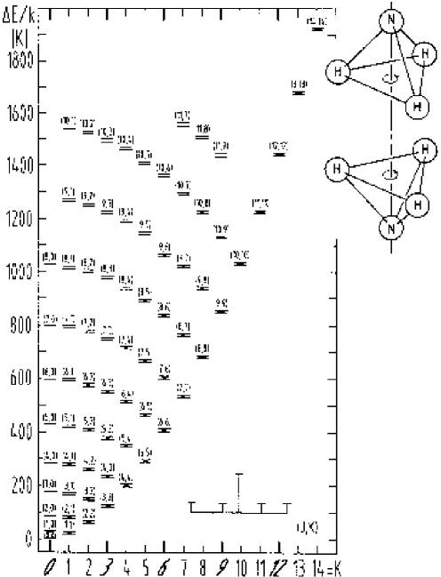
Figure 17: The energy-level diagram of the vibrational ground state of NH₃, a prolate symmetric top molecule. Ortho-NH₃ has $K=0,3,6,9,\cdots$, while para-NH₃ has all other $K$ values (see text). Rotational transitions with $\Delta J=1,\Delta K=0$, give rise to lines in the far IR. This molecule also has transitions with $\Delta J=0,\Delta K=0$ between inversion doublet levels. The interaction of the nuclear spin of ¹⁴N with the electrons causes quadrupole hyperfine structure. In the $\Delta J=0,\Delta K=0$ transitions, the line is split into 5 groups of components. A sketch of the structure of the groups of hyperfine components of the $(J,K)=(1,1)$ inversion doublet line is indicated in the lower right; the separation is of order of MHz. In the upper right is a sketch of the molecule before and after an inversion transition, which gives rise to a 1.3 cm photons RW4 .

Differences in the orientation of the nuclei can be of importance. If a reflection of all particles about the center of mass leads to a configuration which cannot be obtained by a rotation of the molecule, so these reflections represent two different states. For NH₃, we show this situation in the upper part of Fig. 17. Then there are two separate, degenerate states which exist for each value of $(J,K)$ for $J\geq 1$. (The $K=0$ ladder is an exception because of the Pauli principle.) These states are doubly degenerate as long as the potential barrier separating the two configurations is infinitely high. However, in molecules such as NH₃ the two configurations are separated only by a small potential barrier. This gives rise to a measurable splitting of the degenerate energy levels, which is referred to as inversion doubling. For NH₃, transitions between these inversion doublet levels are caused by the quantum mechanical tunneling of the nitrogen nucleus through the plane of the three protons. The wavefunctions of the two inversion doublet states have opposite parities, so that dipole transitions are possible. Thus dipole transitions can occur between states with the same $(J,K)$ quantum numbers. The splitting of the $(J,K)$ levels for NH₃ shown in Fig. 17 is exaggerated; the inversion transitions give rise to spectral lines in the wavelength range near 1 cm. For CH₃CCH or CH₃CN, the splitting caused by inversion doubling is very small since the barrier is much higher than for NH₃.

The direction of the dipole moment of symmetric top molecules is parallel to the $K$ axis. Spectral line radiation can be emitted only by a changing dipole moment. Since radiation will be emitted perpendicular to the direction of the dipole moment, there can be no radiation along the symmetry axis. Thus the $K$ quantum number cannot change in dipole radiation, so allowed dipole transitions cannot connect different $K$ ladders. The different $K$ ladders are connected by octopole radiative transitions which require $\Delta K=\pm 3$. These are very slow, however, and collisions are far more likely to cause an exchange of population between different $K$ ladders. This is used to estimate $T_{\rm K}$ from the ratio of populations of different $(J,K)$ states in symmetric top molecules.

12.6.4 Line Intensities and Column Densities

The extension of this analysis to symmetric top molecules is only slightly more complex. The dipole moment for an allowed transition between energy level $J+1,K$ and $J,K$ for a symmetric top such as CH₃CN or CH₃C₂H is

$$|\mu_{JK}|^{2}=\mu^{2}\,\frac{(J+1)^{2}-K^{2}}{(J+1)(2J+3)}\qquad{\rm for}\quad(J+1,K)\to(J,K)\,.$$ (185)

For these transitions, $J\geq K$ always.

For NH₃, the most commonly observed spectral lines are the inversion transitions at 1.3 cm between levels $(J,K)$ and $(J,K)$. The dipole moment is

$$|\mu_{JK}|^{2}=\mu^{2}\,\frac{K^{2}}{J(J+1)}\qquad{\rm for}\quad\Delta J=0,\,\Delta K=0\,.$$ (186)

When these relations are inserted in (163), the population of a specific level can be calculated following (167). If we follow the analysis used for CO, we can use the LTE assumption to obtain the entire population

$$N({\rm total})=N(J,K)\,\frac{Z}{(2J+1)\,S(J,K)}\,\exp\left[\frac{W(J,K)}{k\,T}\right]\,,$$ (187)

where $W$ is the energy of the level above the ground state, and the nuclear spin statistics are accounted for through the factor $S(J,K)$ for the energy level corresponding to the transition measured. For symmetric top molecules, we have, using the expression for the energy of the level in question (184),

$$N({\rm total})=\frac{Z\,N(J,K)}{(2J+1)\,S(J,K)}\exp\left[\frac{BJ(J+1)+(C-B)K^{2}}{k\,T}\right]\,.$$ (188)

For prolate tops, $A$ replaces $C$ in (188), and in (12.6.4) to (193). If we sum over all energy levels, we obtain $N$(total), the partition function, $Z$ in the following:

$$Z=\sum_{J=0}^{\infty}\sum_{K=0}^{K=J}\,(2J+1)\,S(J,K)\,\exp\left[-\frac{BJ(J+1)+(C-B)K^{2}}{k\,T}\right]\,.\kern-100.0pt$$

If the temperature is large compared to the spacing between energy levels, one can replace the sums by integrals, so that:

$$Z\approx\sqrt{\frac{\pi(k\,T)^{3}}{h^{3}\,B^{2}\,C}}\,.$$ (190)

If we assume that $h\nu\ll kT$, use CGS units for the physical constants, and GHz for the rotational constants $A$, $B$ and $C$, the partition function, $Z$, becomes

$$Z\approx 168.7\,\sqrt{\frac{T^{3}}{B^{2}\,C}}\,.$$ (191)

Substituting into (12.6.4), we have:

$$N({\rm total})=N(J,K)\,\frac{\displaystyle 168.7\,\sqrt{\frac{T^{3}}{B^{2}\,C}}}{(2J+1)\,S(J,K)}\,\exp\left[\frac{W(J,K)}{k\,T}\right]\,.$$ (192)

Here, $N(J,K)$ can be calculated from (167) or (168), using the appropriate expressions for the dipole moment, (186), in the Einstein $A$ coefficient relation, (163) and $W$ is the energy of the level above the ground state. In the ISM, ammonia inversion lines up to (J,K)=(18,18) have been detected WILNH3 .

We now consider a situation in which the NH₃ population is not thermalized. This is typically the case for dark dust clouds. We must use some concepts presented in the next few sections for this analysis. If $n$(H₂)$\sim 10^{4}$ cm^-3, and the infrared field intensity is small, a symmetric top molecule such as NH₃ can have a number of excitation temperatures. The excitation temperatures of the populations in doublet levels are usually between 2.7 K and $T_{\rm K}$. The rotational temperature, T_rot, which describes populations for metastable levels ($J=K$) in different $K$ ladders, is usually close to $T_{\rm K}$. This is because radiative transitions between states with a different K value are forbidden to first order. The excitation temperature which describes the populations with different $J$ values within a given $K$ ladder will be close to 2.7 K, since radiative decay with $\Delta$K=0, $\Delta$J=1 is allowed. Then the non–metastable energy levels, $(J>K)$, are not populated. In this case, $Z$ is simply given by the sum over the populations of metastable levels:

$$Z(J=K)$$ (193)

$$= \sum_{J=0}^{\infty}\,(2J+1)\,S(J,K=J)\,\exp\left[-\frac{BJ(J+1)+(C-B)J^{2}}{k\,T}\right]\,.$$

For the NH₃ molecule in dark dust clouds, where $T_{\rm K}=10$ K and $n$(H₂)$=10^{4}$ cm^-3, we can safely restrict the sum to the three lowest metastable levels:

$$Z(J=K)\approx N(0,0)+N(1,1)+N(2,2)+N(3,3)\,.$$ (194)

Substituting the values for NH₃ metastable levels:

$$Z(J=K)$$

$$\approx N(1,1)\left[\frac{1}{3}\exp\left(\frac{23.1}{k\,T}\right)+1+\frac{5}{3}\exp\left(-\frac{41.2}{k\,T}\right)+\frac{14}{3}\exp\left(-\frac{99.4}{k\,T}\right)\right]\,.\kern-100.0pt$$

For NH₃ we have given two extreme situations: in the first case, described by (12.6.4), is a low-density cloud for which only the few lowest metastable levels are populated. The second case is the LTE relation, given in (192). This represents a cloud in which the populations of the molecule in question are thermalized. More complex are those situations for which the populations of some of the levels are thermalized, and others not. Such a situation requires the use of a statistical equilibrium or an LVG model.

12.7 Asymmetric Top Molecules

12.7.1 Energy Levels

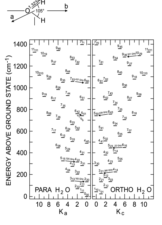
Figure 18: Energy level diagrams for ortho- and para-H₂O. This is an asymmetric top molecule, with the dipole moment along the $B$ axis, that is, the axis with an intermediate moment of inertia. Because of the two identical nuclei, the energy level diagram is split into ortho and para, that show almost no interaction under interstellar conditions. The transitions marked by arrows are well-known masers DELUC , RW4 .

For an asymmetric top molecule there are no internal molecular axes with a time-invariable component of angular momentum. So only the total angular momentum is conserved and we have only $J$ as a good quantum number. The moments of inertia about each axis are different; the rotational constants are referred to as $A,B$ and $C$, with $A>B>C$. The prolate symmetric top ($B=C$) or oblate symmetric top ($B=A$) molecules can be considered as the limiting cases. But neither the eigenstates nor the eigenvalues are easily expressed in explicit form. Each of the levels must be characterized by three quantum numbers. One choice is $J_{{K_{a}}{K_{c}}}$, where $J$ is the total angular momentum, $K_{a}$ is the component of $J$ along the $A$ axis and $K_{c}$ is the component along the $C$ axis. If the molecule is a prolate symmetric top, $J$ and $K_{a}$ are good quantum numbers; if the molecule were an oblate symmetric top, $J$ and $K_{c}$ would be good quantum numbers. Intermediate states are characterized by a superposition of the prolate and oblate descriptions. In Fig. 19, we show the energy level diagram for the lower levels of H₂CO, which is almost a prolate symmetric top molecule with the dipole moment along the $A$ axis. Since radiation must be emitted perpendicular to the direction of the dipole moment, for H₂CO there can be no radiation emitted along the $A$ axis, so the quantum number $K_{a}$ will not change in radiative transitions.

12.7.2 Spin Statistics and Selection Rules

The case of a planar molecule with two equivalent nuclei, such as H₂CO, shows is a striking illustration of these effects (see Fig. 19). The dipole moment lies along the $A$ axis. A rotation by $180^{\rm o}$ about this axis will change nothing in the molecule, but will exchange the two protons. Since the protons are fermions, this exchange must lead to an antisymmetric wavefunction. Then the symmetry of the spin wave function and the wave function describing the rotation about the $A$ axis must be antisymmetric. The rotational symmetry is $(-1)^{K_{a}}$. If the proton spins are parallel, that is ortho-H₂CO, then the wave function for $K_{a}$ must be anti-symmetric, or $K_{a}$ must take on an odd value. If the proton spins are anti-parallel, for para-H₂CO, $K_{a}$ must have an even value (Fig. 19). For ortho-H₂CO, the parallel spin case, there are three possible spin orientations. For para-H₂CO, there is only one possible orientation, so the ratio of ortho-to-para states is three. Such an effect is taken into account in partition functions (175) by spin degeneracy factors, which are denoted by the symbol $S(J,K)$. For ortho-H₂CO, $S(J,K)=3$, for para-H₂CO, $S(J,K)=1$. This concept will be applied in Sect. 12.7.3.

Allowed transitions can occur only between energy levels of either the ortho or the para species. For example, the 6 cm H₂CO line is emitted from the ortho-modification only (see Fig. 19). Another example is the interstellar H₂O maser line at $\lambda=1.35$ cm which arises from ortho-H₂O (see Fig. 18). The H₂O molecule is a more complex case since the dipole moment is along the $B$ axis. Then in a radiative transition, both $K_{a}$ and $K_{c}$ must change between the initial and final state.

12.7.3 Line Intensities and Column Densitiess

For asymmetric molecules the moments of inertia for the three axes are all different; there is no symmetry, so three quantum numbers are needed to define an energy level. The relation between energy above the ground state and quantum numbers is given in Appendix IV of TOWNES or in databases for specific molecules (see figure captions for references). The relation for the dipole moment of a specific transition is more complex; generalizing from (163), we have, for a spontaneous transition from a higher state, denoted by $u$ to a lower state, denoted by $l$:

$$A=1.165\times 10^{-11}\,\nu^{3}_{\rm x}\,\mu_{x}^{2}\,\frac{{\cal S}(u;l)}{2J^{\prime}+1}\,.$$ (196)

This involves a dipole moment in a direction $x$. As before, the units of $\nu$ are GHz, and the units of $\mu$ are Debyes (i. e., 1 Debye $=10^{-18}$ times the e.s.u. value). The value of the quantum number $J^{\prime}$ refers to the lower state. The expression for ${\cal S}(u;l)$, the line strength is an indication of the complexity of the physics of asymmetric top molecules. The expression ${\cal S}(u;l)$ is the angular part of the dipole moment between the initial and final state. The dipole moment can have a direction which is not along a single axis. In this case there are different values of the dipole moment along different molecular axes. In contrast, for symmetric top or linear molecules, there is a dipole moment for rotational transitions. Methods to evaluate transition probabilities for asymmetric molecules are discussed at length in TOWNES . There is a table of ${\cal S}(u;l)$ in their Appendix V. We give references for ${\cal S}(u;l)$ in our figure captions. From the expression for the Einstein $A$ coefficient, the column density in a given energy level can be related to the line intensity by (167). Following the procedures used for symmetric top molecules, we can use a relation similar to (12.6.4) to sum over all levels, using the appropriate energy, $W$, of the level $J_{K_{a}K_{c}}$ above the ground state and the factor $S(J_{K_{a}K_{c}})$ for spin statistics:

$$N({\rm total})=N(J_{K_{a}K_{c}})\,\frac{Z}{(2J+1)\,S(J_{K_{a}K_{c}})}\,\exp\left(\frac{W}{k\,T}\right)\,.$$ (197)

If the populations are in LTE, one can follow a process similar to that used to obtain (191). Then we obtain the appropriate expression for the partition function:

$$Z=168.7\,\sqrt{\frac{T^{3}}{A\,B\,C}}\,.$$ (198)

When combined with the Boltzmann expression for a molecule in a specific energy level, this gives a simple expression for the fraction of the population in a specific rotational state if LTE conditions apply:

$$N({\rm total})\approx N(J_{K_{a}K_{c}})\,\frac{168.7\,\displaystyle\sqrt{\frac{T^{3}}{A\,B\,C}}}{(2J+1)\,S(J_{K_{a}K_{c}})}\,\exp\left(\frac{W}{k\,T}\right)\,.$$ (199)

In this expression, $S(J_{K_{a}K_{c}})$ accounts for spin statistics for energy level $J_{K_{a}K_{c}}$, and $A$, $B$ and $C$ are the molecular rotational constants in GHz. $W$, the energy of the level above the ground state, and $T$, the temperature, are given in Kelvin. Given the total molecular column density and the value of $T$, the feasibility of detecting a specific line can be obtained when the appropriate $A$ coefficient value is inserted into (167) or (168).

As pointed out in connection with NH₃, $T$ need not be $T_{\rm K}$. In reality, a number of different values of $T$ may be needed to describe the populations. We will investigate the influence of excitation conditions on molecular populations and observed line intensities next.

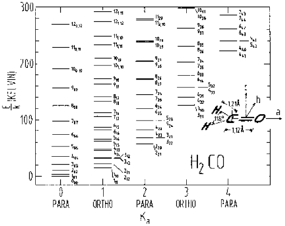
Figure 19: Energy-level diagram of formaldehyde, H₂CO. This is a planar asymmetric top, but the asymmetry is very small. The energy-level structure is typical of an almost prolate symmetric top molecule. In the lower right is a sketch of the structure of the molecule MANGUM

Two important interstellar molecules are H₂CO and H₂O. Here we summarize the dipole selection rules. Rotating the molecule about the axis along the direction of the dipole moment, we effectively exchange two identical particles. If these are fermions, under this exchange the total wavefunction must be antisymmetric. For H₂CO, in Sect. 12.6.2 we reviewed the spin statistics. Since the dipole moment is along the A axis, a dipole transition must involve a change in the quantum numbers along the B or C axes. From Fig. 19, the K_a=0 ladder is para-H₂CO, so to have a total wavefunction which is antisymmetric, one must have a space wavefunction which is symmetric. For a dipole transition, the parities of the initial and final states must have different parities. This is possible if the C quantum number changes. For H₂O, the dipole moment is along the B axis, from Fig. 18. In a dipole transition, the quantum number for the B direction will not change. For ortho-H₂O, the spin wavefunction is symmetric, so the symmetry of the space wavefunction must be antisymmetric. In general, this symmetry is determined by the product of K_a and K_c. For ortho-H₂O, this must be K_aK_c=(odd)(even), i.e. $oe$, or $eo$. For allowed transitions, one can have $oe-eo$ or $eo-oe$. For para-H₂O, the rule is $oo-ee$ or $ee-oo$. Clearly H₂S follows the selection rules for H₂O. These rules will be different for SO₂ since the exchanged particles are bosons. More exotic are D₂CO, ND₃ and D₂O.

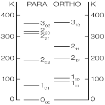
Figure 20: The few lowest energy levels of the H₂D⁺ molecule. This is a planar, triangular-shaped asymmetric top GERLICH .

The species H${}_{3}^{+}$ has the shape of a planar triangle. It is a key to ion-molecule chemistry, but has no rotational transitions because of its symmetry. The deuterium isotopomer, H₂D⁺ is an asymmetric top molecule with a permanent dipole moment. The spectral line from the 1₁₀-1₁₁ levels ortho species was found at 372.421 GHz. A far infrared absorption line from the 2₁₂-1₁₁ levels was also detected. We show an energy level diagram in Fig. 20. The doubly deuterated species, D₂H⁺,has been detected in the 1₁₀-1₀₁ line at 691.660 GHz from the para species (see VASTEL ).

12.8 Electronic Angular Momentum

In many respects the description of electronic angular momentum is similar to that of atomic fine structure as described by Russell-Saunders ($L\,S$) coupling. Each electronic state is designated by the symbol ${}^{2S+1}\Lambda_{\Omega}$, where $2S+1$ is the multiplicity of the state with $S$ the electron spin and $\Lambda$ is the projection of the electronic orbital angular momentum on the molecular axis in units of $\hbar$. The molecular state is described as $\Sigma,\Pi,\Delta$ etc., according to whether $\Lambda=0,1,2,\dots\;.$

$\Sigma$ is the projection of the electron spin angular momentum on the molecular axis in units of $\hbar$ (not to be confused with the symbol $\Sigma$, for $\Lambda=0$). Finally, $\Omega$ is the total electronic angular momentum. For the Hund coupling case A, $\Omega=|\Lambda+\Sigma|$ [see e. g. RW4 ].

Since the frequencies emitted or absorbed by a molecule in the optical range are due to electronic state changes, many of the complications found in optical spectra are not encountered when considering transitions in the cm and mm range. However the electronic state does affect the vibrational and rotational levels even in the radio range. For most molecules, the ground state has zero electronic angular momentum, that is, a singlet sigma, ${}^{1}\Sigma$ state. For a small number of molecules such as OH, CH, C₂H, or C₃H, this is not the case; these have ground state electronic angular momentum. Because of this fact, the rotational energy levels experience an additional energy-level splitting, which is $\Lambda$ doubling. This is a result of the interaction of the rotation and the angular momentum of the electronic state. This splitting causes the degenerate energy levels to separate. This splitting can be quite important for $\Pi$ states; for $\Delta$ and higher states it is usually negligible. The OH molecule is a prominent example for this effect. Semi-classically, the $\Lambda$ doubling of OH can be viewed as the difference in rotational energy of the (assumed rigid) diatomic molecule when the electronic wave function is oriented with orbitals in a lower or higher moment of inertia state. We show a sketch of this in the upper part of Fig. 21. Since the energy is directly proportional to the total angular momentum quantum number and inversely proportional to the moment of inertia, the molecule shown on the left has higher energy than the one shown on the right.

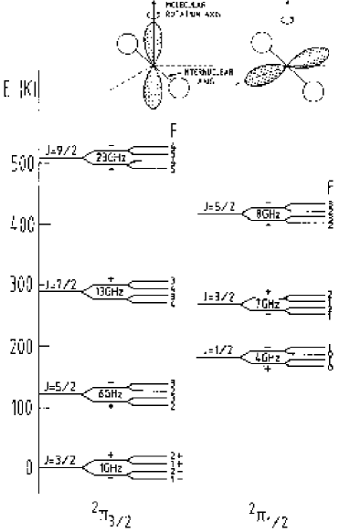
Figure 21: The lower energy levels of OH showing $\Lambda$-doubling. $F$ is the total angular momentum, including electron spin, while $J$ is the rotational angular momentum due to the nuclear motion. The quantum number $F$ includes hyperfine splitting of the energy levels. The parities of the states are also shown under the symbol $F$. The $\Lambda$ doubling causes a splitting of the $J$ states. In the sketch of the OH molecule, the shaded regions represent the electron orbits in the $\Lambda$ state. The two unshaded spheres represent the O and H nuclei. The configuration shown on the left has the higher energy RW4 .

There are also a few molecules for which the orbital angular momentum is zero, but the electron spins are parallel, so that the total spin is unity. These molecules have triplet sigma ${}^{3}\Sigma$ ground states. The most important astrophysical example is the SO molecule; another species with a triplet $\Sigma$ ground state is O₂. These energy levels are characterized by the quantum number, $N$, and the orbital angular momentum quantum number $J$. The most probable transitions are those within a ladder, with $\Delta J=\Delta N=\pm 1$, but there can be transitions across $N$ ladders. As with the OH molecule, some states of SO are very sensitive to magnetic fields. One could then use the Zeeman effect to determine the magnetic field strength. This may be difficult since a 1 $\mu$Gauss field will cause a line splitting of only about 1 Hz in linear polarization. Even so, measurements of the polarization of the $J_{N}=1_{0}-0_{1}$ line of SO (RW4 ) may allow additional determinations of interstellar magnetic fields.

12.8.1 Molecules with Hindered Motions

The most important hindered motion involve quantum mechanical tunneling; such motions cannot occur in classical mechanics because of energy considerations. A prime example of this phenomenon is the motion of the hydrogen atom attached to oxygen in CH₃OH, methanol. This H atom can move between 3 positions between the three H atoms in the CH₃ group. Another example is motion of the CH₃ group in CH₃COOH, methyl formate. These are dependent on the energy. At low energy these motions do not occur, while at larger energies are more important. For both methanol and methyl formate these motions allow a large number of transitions in the millimeter and sub-millimeter range.

The description of energy levels of methyl formate follows the standard nomenclature. For methanol, however, this is not the case, due to historical developments. These energy levels are labelled as $J_{k}$, where $K$ can take on both positive and negative values as in Fig.  22. There is a similar scheme for naming energy levels of A type methanol, as $A^{\pm}_{k}$. A and E type methanol are analogous to ortho and para species, in that these states are not normally coupled by collisions.

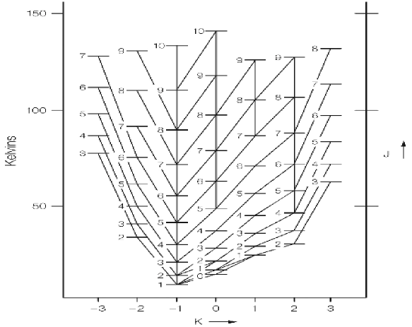
Figure 22: Energy-level diagram of E type methanol, CH₃OH. This is an asymmetric top. The energy-level structure is typical of an almost prolate symmetric top molecule. The lines connecting the levels show the spontaneous transitions with the largest A coefficients from eac level; where the two largest A coefficients are within a factor of 2, both transitions are shown RW5 .

Torsionally excited states of methanol have been found in the interstellar medium. These are analogous to transitions from vibrationally excited states to the ground state of a molecule. Another complexity is that because of its structure, there are two dipole moments, along either the c or the a axis

13 Astronomical Applications

In the following, methods to deterimine the parameters of molecular clouds are summarized

13.1 Kinetic Temperatures

A crucial input parameter for the LVG calculations is $T_{\rm K}$. Linewidths of thermally excited species provide a definite value for $T_{\rm K}$ if the turbulent velocity can be neglected. The relation is

$$T_{\rm k}=21.2\left({m/m}_{\rm H}\right)\,\left(\mbox{\greeksym{D}}{V}_{\rm t}\right)^{2}$$

where $m$ is the molecule, $m_{H}$ is the mass of hydrogen, and $\mbox{\greeksym{D}}{V}_{\rm t}$ is the FWHP thermal width. Such a relation has been applied to NH₃ lines (with success!) in quiescent dust clouds.

Historically, $T_{\rm K}$ was obtained at first from the peak intensities of rotational transitions of CO, which has a small spontaneous decay rate. From the ratio of CO to ¹³CO line intensities, $\tau({\rm CO})\gg 1$. After correcting for cloud size, from (172) $T_{\rm MB}$ and $T_{\rm ex}$ are directly related. In addition, the large optical depths reduce the critical density by a factor $\tau$, the line optical depth, so that for the $J=1\to 0$ line, the value of the critical density $n^{*}\approx 50$ cm^-3. Then, the level populations are determined by collisions, so the excitation temperature for the $J=1\to 0$ transition is $T_{\rm K}$. Usually, it is assumed that the beam filling factor is unity; for distant clouds or external galaxies, the filling factor is clearly less.

An alternative to CO measurements makes use of the fact that radiative transitions between different $K$ ladders in symmetric top molecules are forbidden. Then the populations of the different $K$ ladders are determined by collisions. Thus a method of determining $T_{\rm K}$ is to use the ratio of populations in different $K$ ladders of molecules such as NH₃ at 1.3 cm, or CH₃CCH and CH₃CNin the mm/sub-mm range. This is also approximately true for different $K_{a}$ ladders of H₂CO. Since ratios are involved, beam filling factors play no role. Even for extended clouds, $T_{\rm k}$ values from CO and NH₃ may not agree. This is because NH₃ is more easily dissociated so must arise from the cloud interior. Thus for a cloud heated externally, the $T_{\rm k}$ from CO data will be larger than that from NH₃.

For NH₃, the rotational transitions, $(J+1,K)\rightarrow(J,K)$, occur in the far infrared and have Einstein $A$ coefficients of order 1 s^-1; for inversion transitions, A values are $\sim 10^{-7}$ s^-1 (see, e. g., Table 2). These non metastable states require extremely high H₂ densities or intense far infrared fields to be populated. Thus NH₃ non metastable states ($J>K$) are not suitable for $T_{\rm K}$ determinations. Rather, one measures the inversion transitions in different metastable ($J=K$) levels. Populations cannot be transferred from one metastable state to another via allowed radiative transitions. This occurs via collisions, so the relative populations of metastable levels are directly related to $T_{\rm K}$. The column densities are obtained from the inversion transitions from different metastable states, and convert these to column densities using (167) to (170). If the NH₃ lines are optically thick, one can use the ratios of satellite components to main quadrupole hyperfine components, in most cases, to determine optical depths. A large number of $T_{\rm K}$ determinations have been made using NH₃ in dark dust clouds. Usually these involve the ($J,K$)=(1,1) and (2,2) inversion transitions.

13.2 Linewidths, Radial Motions and Intensity Distributions

From the spectra themselves, the linewidths, $\Delta{\rm V}_{1/2}$, and radial velocities, V_lsr, give an estimate of motions in the clouds. The $\Delta{\rm V}_{1/2}$  values are a combination of thermal and turbulent motions. Observations show that the widths are supersonic in most cases. In cold dense cores, motions barely exceed Doppler thermal values. Detailed measurements of lines with moderate to large optical depths show that the shapes are nearly Gaussian. However, simple models in which unsaturated line shapes are Gaussians would give flat topped shapes at high optical depths. This is not found. More realistic models of clouds are those in which shapes are determined by the relative motion of a large number of small condensations, or clumps, which emit optically thick line radiation. If the motions of such small clumps are balanced by gravity, one can apply the virial theorem. Images of isolated sources can be used for comparing with models. One example is the attempt to characterize the kinetic temperature and the H₂ density distributions from spectral line or thermal dust emission data.

13.3 Determinations of H₂ Densities

If a level is populated by collisions with H₂, the main collision partner, a first approximation to the H₂ density can be had if one sets the collision rate, $n({\rm H}_{2})\langle\sigma\,v\rangle$ equal to the $A$ coefficient. The brackets indicate an average over velocities of H₂, which are assumed to be Boltzmann distributed. The H₂ density for a given transition which will bring $T_{\rm ex}$ midway between the radiation temperature and $T_{\rm K}$ is referred to as the critical density, and is denoted by $n^{*}$. That is $n^{*}\langle\sigma\,v\rangle=A$. However, this can be at best only an approximate estimate. For reliable determination of H₂ densities n(H₂) one must measure at least two spectral lines of a given species, estimates of the kinetic temperature, collision rates, and a radiative transport model. One can assume that the lines are optically thin, and use a statistical equilibrium model, but the present approach is to apply the LVG model RW4 . Clearly, the more lines measured, the more reliable the result. For linear molecules such as CO or CS, it is not possible to separate kinetic temperature and density effects. For example, CO with $T_{\rm K}$=10K will have a J=2-1 line much weaker than the J=1-0 line no matter how high the density. However, if the plot of normalized CO column density versus energy above the ground state shows a turn over, that is a decrease in intensity, it is possible to find a unique combination of $T_{\rm K}$ and n(H₂).

13.4 Cloud Masses

13.4.1 Virial Masses

If we assume that only gravity is to be balanced by the motions in a cloud, then, for a uniform density cloud of radius $R$, in terms of the line of sight FWHP velocity, virial equilibrium requires:

$$\framebox{$\displaystyle\frac{M}{M_{\odot}}=250\left(\frac{\Delta v_{1/2}}{{\rm km\,s}^{-1}}\right)^{2}\left(\frac{R}{{\rm pc}}\right)$}\quad.$$ (200)

Once again very optically thick lines should not be used in determining masses using (200).

Another probe of such regions is thermal emission from dust (117). Given the dust temperature, such data allow one to derive H₂ abundances and cloud masses.

13.4.2 Masses from Measurements of CO and ¹³CO

CO is by far the most widespread molecule with easily measured transitions. The excitation of CO is close to LTE and the chemistry is thought to be ”well understood”, so measurements of CO and CO isotopomers (and dust emission measurments!) are the most important tool(s) for estimating masses of molecular clouds.

Even if all of the concepts presented in this section are valid, there may be uncertainties in the calculation of the column densities of CO. These arise from several sources which can be grouped under the general heading non-LTE effects. Perhaps most important is the uncertainty in the excitation temperature. While the ¹²CO emission might be thermalized even at densities $<100$ cm^-3, the less abundant isotopes may be sub-thermally excited, i.e., populations characterized by $T_{\rm ex}<T_{\rm K}$. (this can be explained using the LVG approximation (137)). Alternatively, if the cloud in question has no small scale structure, ¹³CO emission will arise primarily from the cloud interior, which may be either hotter or cooler than the surface; the optically thick ¹²CO emission may only reflect conditions in the cloud surface. Another effect is that, although $T_{\rm ex}$ may describe the population of the $J=0$ and $J=1$ states well, it may not for $J>1$. That is, the higher rotational levels might not be thermalized because their larger Einstein $A$ coefficients lead to a faster depopulation. This lack of information about the population of the upper states leads to an uncertainty in the partition function. Measurements of other transitions and use of LVG models allow better accuracy. For most cloud models, LTE gives overestimates of the true ¹³CO column densities by factors from 1 to 4 depending on the properties of the model and of the position in the cloud. Thus a factor of $\sim$ two uncertainties should be expected when using LTE models. The final step to obtain the H₂ column density is to assume a ratio of CO to H₂. This is generally taken to be 10^-4. In spite of all these uncertainties, one most often attempts to relate measurements of the CO column density to that of H₂; estimates made using lines of CO (and isotopomers) are probably the best method to obtain the H₂ column density and mass of molecular clouds.

An LVG treatment of the dependence of the total column density on the line intensity of the $J=2\to 1$ line shows that a simple relation is valid for $T_{\rm K}$ from 15 K to 80 K, and $n$(H₂) from $\sim 10^{3}$ to $\sim 10^{6}$ cm^-3. An assumption used in obtaining this relation is that the ratio of C¹⁸O to H₂ is $1.7\times 10^{-7}$, which corresponds to (C/H₂) $=10^{4}$, and (¹⁶O/¹⁸O) $=500$. The latter ratio is obtained from isotopic studies for molecular clouds near the Sun. Then we have

$$N_{\rm H_{2}}=2.65\times 10^{21}\,\int T_{\rm MB}({\rm C}^{18}{\rm O},J=2\to 1){\rm\,d}v\,.$$ (201)

The units of $v$ are km s^-1, of $T_{\rm MB}$(C¹⁸O, $J=2\to 1$) are Kelvin, and of $N_{\rm H_{2}}$ are cm^-2. This result can be used to determine cloud masses, if the distance to the cloud is known, by a summation over the cloud, position by position, to obtain the total number of H₂.

The total cloud masses obtained from the methods above, or similar methods, is sometimes referred to as the ’CO mass’; this terminology can be misleading, but is frequently found in the literature.

13.4.3 Masses from the X Factor

In large scale surveys of the CO $J=1\to 0$ line in our galaxy and external galaxies, it has been found, on the basis of a comparison of CO with ¹³CO  maps, that the CO integrated line intensities measure mass, even though this line is optically thick. The line shapes and intensity ratios along different lines of sight are remarkably similar for both ¹²CO and ¹³CO line radiation. This can be explained if the total emission depends primarily on the number of clouds. If so, ¹²CO line measurements can be used to obtain estimates of $N_{\rm CO}^{12}$. Observationally, in the disk of our galaxy, the ratio of these two quantities varies remarkably little for different regions of the sky.

This empirical approach has been followed up by a theoretical analysis. The basic assumption is that the clouds are virial objects, with self-gravity balancing the motions. If these clouds are thought to consist of a large number of clumps, each with the same temperature, but sub thermally excited (i. e., $T_{\rm ex}<T_{\rm K}$), then from an LVG analysis of the CO excitation, the peak intensity of the CO line will increase with $\sqrt{n({\rm H_{2}})}$, and the linewidth will also increase by the same factor, as can be seen from (200). The exact relation between the integrated intensity of the CO $J=1\to 0$ line and the column density of H₂ must be determined empirically. Such a relation has also been applied to other galaxies and the center of our galaxy. However, the environment, such as the ISRF, may be very different and this may have a large effect on the cloud properties. For the disk of our galaxy, a frequently used conversion factor is:

$$N_{\rm H_{2}} = X\int T_{\rm MB}({\rm CO},J=1\to 0){\rm\,d}v$$ (202)

$$= 2.3\times 10^{20}\int T_{\rm MB}({\rm CO},J=1\to 0){\rm\,d}v\,.$$

where $X=2.3\times 10^{20}$ and $N_{\rm H_{2}}$ is in units of cm^-2. By summing the intensities over the cloud, the mass in M_⊙ is obtained. Strictly speaking, this relation is only valid for whole clouds. The exact value of the conversion factor between CO integrated line intensity and mass, $X$, is a matter of some dispute.

13.5 Additional Topics

13.5.1 Freezing Out on Grain Surfaces

For H₂ densities $>10^{6}$ cm^-3, one might expect a freezing out of molecules onto grains for cold, dense regions. From a simplified theory for H₂ densities $>10^{6}$ cm^-3, the time for a molecule-grain collision is 3000 years, short compared to other time scales. Then CO and most other molecules might be condensed out of the gas phase, so that spectroscopic measurements cannot be used as a probe of very dense regions. Empirically N₂H⁺, NH₃ and H₂D⁺ appear to remain in the gas phase even at low kinetic temperatures and high densities.

13.5.2 Self Shielding of CO

As is well established, CO is dissociated by line radiation. Since the optical depth of CO is large, this isotopomer will be self-shielded. If there is no fine spatial structure, selective dissociation will cause the extent of ¹²CO to be greater than that of ¹³CO, which will be greater than the extent of C¹⁸O.

References

- (1) W.J. Altenhoff et al: Veroeff. Sternwarte Bonn, 59 (1960)
- (2) W.J. Altenhoff (1985): The Solar System: (Sub)mm continuum observations in ESO Conf & Workshop Proc No 22 ed by P. Shaver, K. Kjar, (European Southern Obs., Garching) p. 591
- (3) J. W. M. Baars: The Parabolic Reflector Antenna in Radio Astronomy and Communication Astrophysics Space Science Library (Springer, Berlin, Heidelberg, New York 2007)
- (4) D. S. Balser et al: Ap. J. 430, 667 (1994)
- (5) R. Bachiller, J. Cernicharo ed: Science with the Atacama Large Millimeter Array: A New Era for Astrophysics (Springer, Berlin Heidelberg New York 2008)
- (6) A. J. Baker, J. Glenn, A. I. Harris, J. G. Mangum, M. S. Yun, eds: From Z Machines to ALMA: (Sub)millimeter Spectroscopy of Galaxies Conf. Ser. 75 (Astron Soc of Pacific, San Francisco 2007)
- (7) R. N. Bracewell The Fourier Transform and its Application, 2nd ed. (McGraw Hill, New York 1986)
- (8) T. Cornwell, E. B. Fomalont: Self Calibration in Synthesis Imaging in Radio Astronomy, Conf Series vol 6, ed by R. Perley et al. (Publ. Astron.Soc. Pacific, San Francisco 1989) p. 185
- (9) F. J. DeLucia, P. Helminger, W. H. Kirchoff J: Phys Chem Ref Data 3, 21 (1972)
- (10) R. H. Dicke: Rev. Sci. Instrum. 17, 268 (1946)
- (11) D. Downes: Radio Telescopes: Basic Concepts in Diffraction-Limited Imaging with Very Large Telescopes, NATO ASI Series vol 274, ed by D. M. Alloin, J. M. Mariotti (Kluwer, Dordrecht 1989) p. 53
- (12) A. Dutrey ed: IRAM Millimeter Interferometry Summer School 2 (IRAM, Grenoble, France 2000)
- (13) E. Krügel: The Physics of Interstellar Dust (Inst. of Physics Press, Bristol UK 2002)
- (14) D. Gerlich F. Windisch, P. Hlavenka, R. Plasil, J. Glosik: Phil. Trans. R. Soc. A 364, 3007 (2006)
- (15) P. F. Goldsmith ed: Instrumentation and Techniques for Radio Astronomy (IEEE Press, New York 1988)
- (16) P. F. Goldsmith: Quasioptical Systems: Gaussian Beam Quasioptical Propagation and Applications (Wiley-IEEE Press, New York 1994)
- (17) J. M. Jackson et. al.: Ap. J. Suppl. 163, 145 (2006)
- (18) M. A. Gordon, R. L. Sorochenko: Radio Recombination Lines, Their Physics and Astronomical Applications, Astrophysics and Space Science Library 282, (Kluwer Academic Publications: Dordrecht 2002)
- (19) S. F. Gull, G. J. Daniell: Nature 272, 686 (1978)
- (20) L. Gurvits, S. Frey, S. Rawlings, eds: Radio Astronomy from Karl Jansky to Microjansky (EDP Sciences, Paris 2005)
- (21) E. Herbst: Chemical Society Reviews 30, 168 (2001)
- (22) R. Hildebrand: Quarterly J. Roy. Astron. Soc. 24, 267 (1983)
- (23) J. Högbom, J.: A. & A. Suppl. 15, 417 (1974)
- (24) W. S. Holland et al: MNRAS 303, 659 (1999)
- (25) F. A. Jenkins, H. E. White): Fundamentals of Optics, 4th ed. (McGraw-Hill, New York 2001) Chap. 13
- (26) D. R. Johnson, F. J. Lovas, W. H. Kirchoff: J. Phys. Chem Ref Data 1, 1011 (1972)
- (27) D. Johnstone et al: Ap. J. Supp.131, 505 (2000)
- (28) H. W. Kroto: Molecular Rotation Spectra (Dover, New York 1992)
- (29) J. Lequeux: The Interstellar Medium ( Springer Berlin, Heidelberg, New York 2004)
- (30) A. W. Love ed: Electromagnetic Horn Antennas (IEEE Press, New York 1976)
- (31) J. G. Mangum, A. Wootten: Ap. J. Suppl. 89, 123 (1993)
- (32) D. P. Marrone, J. M. Moran, J.-H. Zhao, R. Rao: Ap. J. 654, L57 (2007)
- (33) J. Martin-Pintado et al: A. & A. 286, 890 (1994)
- (34) P. G. Mezger, J. E. Wink, R. Zylka: A. & A. 228, 95 (1990)
- (35) F. Motte, S. Bontemps, N. Schneider, P. Schilke, K. M. Menten, D. Broguierè: A. & A. 476, 1243 (2006)
- (36) J. L. Pawsey, R. N. Bracewell: Radio Astronomy (Oxford University Press, Oxford 1954)
- (37) Reipurth, B., Jewett, D., Keil, K. eds: Protostars and Planets V (Univ of Arizona Press, Tucson 2007)
- (38) K. Rohlfs, T. L. Wilson: Tools of Radio Astronomy (Springer, Berlin, Heidelberg, New York 2004)
- (39) G. H. Rieke: Detection of Light: From Ultraviolet to the Submillimeter (Cambridge Univ. Press, Cambridge UK 2002)
- (40) G. B. Rybicki, A. P. Lightman: Radiative Processes in Astrophysics (Wiley, New York 1979)
- (41) G. Sandell: MNRAS 271, 75 (1994)
- (42) P. A. G. Scheuer: Radiation in Plasma Astrophysics, ed by P. A. Sturrock, Proc Int Sch Phys Enrico Fermi, 39, (Academic Press, New York 1967) p. 39
- (43) P. M. Solomon,, P. A. vanden Bout: Ann. Rev. A. & A. 43, 677 (2005)
- (44) L. Sparke, J. S. Gallagher III: Galaxies in the Universe: An Introduction (Cambridge Univ. Press, Cambridge UK 2000)
- (45) S. W. Stahler, F. Palla: The Formation of Stars (Wiley-VCH, New York 2005)
- (46) C. Thum, H. Wiesemeyer, G. Paubert, S. Navarro, D. Morris: PASP 120, 777 (2008)
- (47) A. G. G. M. Tielens: The Physics and Chemistry of the Interstellar Medium (Cambridge Univ. Press, Cambridge UK 2005)
- (48) A. R. Thompson, J. M. Moran, G. W. Swenson: Interferometry and Synthesis in Radio Astronomy 2nd ed. (Wiley, New York 2001)
- (49) C. H. Townes, A. H. Schawlow: Microwave Spectroscopy (Dover, New York 1975)
- (50) C. Vastel et al: ApJ645, 1198 (2006)
- (51) T. L. Wilson, S. Huettemeister: Tools of Radio Astronomy: Problems and Solutions (Springer, Berlin, Heidelberg, New York 2005)
- (52) T. L. Wilson, C. Henkel, S. Huettemeister: A& A 460, 533 (2006)
- (53) T. L. Wilson, K. Rohlfs, S. Huettemeister: Tools of Radio Astronomy (Springer, Berlin, Heidelberg, New York 2008)
Index
-
Absorption
- tropospheric §6.1
-
Amplifier
- transistor §4.4
- Angular momentum §12.2, §12.7.1
- Antenna
-
Antennas
- reciprocity §5