Abstract

We provide a new, independent, and analytic estimate of the lowest glueball mass, and we found it at 1661 MeV within a relativistic quantum-field model based on analytic confinement. The conventional mesons and the weak decay constants are described to extend the consideration. For the spectra of two-gluon and two-quark bound states we solve the ladder Bethe-Salpeter equation. By using a minimal set of model parameters (the quark masses, the coupling constant, and the confinement scale) we obtain numerical results which are in reasonable agreement with experimental evidence in the wide range of energy scale. The model serves a reasonable framework to describe simultaneously different sectors in low-energy particle physics.

PACS: 11.10.Lm, 11.10.St, 11.15.Tk, 12.38.Aw, 12.31Mk, 12.39Ki, 14.40.-n

1 Introduction

Confinement and dynamical symmetry breaking are two crucial features of QCD, although they correspond to different energy scales [1, 2]. Confinement is an explanation of the physics phenomenon that color charged particles are not observed; the quarks are confined with other quarks by the strong interaction to form bound states so that the net color is neutral. However, there is no analytic proof that QCD should be color confining and the reasons for quark confinement may be somewhat complicated. There exist different suggestions about the origin of confinement, some dating back to the early eighties (e.g., [3, 4]) and some more recent based on the Wilson loop techniques [5], string theory quantized in higher dimensions [6], and lattice Monte Carlo simulations (e.g., [7]), etc. It may be supposed that the confinement is not obligatory connected with the strong-coupling regime, but it may be induced by the nontrivial background fields. One of the earliest suggestion in this direction is the analytic confinement (AC) based on the assumption that the QCD vacuum is realized by the self-dual vacuum gluon fields which are stable versus local quantum fluctuations and related to the confinement and chiral symmetry breaking [3]. This vacuum gluon field could serve as the true minimum of the QCD effective potential [8]. Particularly, it has been shown that the vacuum of the quark-gluon system has the minimum at the nonzero self-dual homogenous background field with constant strength and the quark and gluon propagators in the background gluon field represent entire analytic functions on the complex momentum plan $p^{2}$ [9]. However, direct use of these propagators for low-energy particle physics problems encounters complex formulae and cumbersome calculations.

We are far from understanding how QCD works at longer distances. The well-established conventional perturbation theory cannot be used at low energy, where the most interesting and novel behavior is expected [10]. The calculations of hadron mass characteristics on the level of experimental data precision still remain among the unsolved problems in QCD due to some technical and conceptual difficulties related with the color confinement and spontaneous chiral symmetry breaking. In such a case, it is useful to investigate the corresponding low-energy effective theories instead of tackling the fundamental theory itself. Although lattice gauge theories are the way to describe effects in the strong-coupling regime, other methods can be applied for some problems not yet feasible with lattice techniques. So data interpretations and calculations of hadron characteristics are frequently carried out with the help of phenomenological models. Different nonperturbative approaches have been proposed to deal with the long distance properties of QCD, such as chiral perturbation theory [11], QCD sum rule [12], heavy quark effective theory [13], etc. Along outstanding advantages these approaches have obvious shortcomings. Particularly, rigorous lattice QCD simulations [14] suffer from lattice artifacts and uncertainties and cannot yet give a reliable result in the low-energy hadronization region. The coupled Schwinger-Dyson equation (SDE) is a continuum method without IR and UV cutoffs and describes successfully the QCD vacuum and the long distance properties of strong interactions such as confinement and chiral symmetry breaking (e.g., [15]). However, an infinite series of equations requires to make truncations which are gauge dependent. The Bethe-Salpeter equation (BSE) is an important tool for studying the relativistic two-particle bound state problem in a field theory framework [16]. The BS amplitude in Minkowski space is singular and therefore, it is usually solved in Euclidean space to find the binding energy. The solution of the BSE allows to obtain useful information about the understructure of the hadrons and thus serves a powerful test for the quark theory of the mesons. Numerical calculations indicate that the ladder BSE with phenomenological potential models can give satisfactory results (for a review, see [17]).

It represents a certain interest to combine the AC conception and the BSE method within a phenomenological model and to investigate some low-energy physics problems by using the path-integral approach. Particularly, it is shown that a “toy” model of interacting scalar “quarks” and “gluons” with AC could result in qualitatively reasonable description of the two- and three-particle bound states [18] and obtained analytic solutions to the ladder BSE lead to the Regge behaviors of meson spectra [19].

Below we consider a more realistic model introduced in [20] by taking into account the spin, color and flavor degrees of constituents. This model was further modified in [21], applied to leptonic decay constants in [22], and used to simultaneously compute meson masses and estimate the mass of the lowest-lying glueball in [23, 24]. Here the aim is to collect all necessary formulae, explain the method in detail, and show that the correct symmetry structure of the quark-gluon interaction in the confinement region reflected in simple forms of the quark and gluon propagators can result in quantitatively reasonable estimates of physical characteristics in low-energy particle physics. In doing so, we build a model describing hadrons as relativistic bound states of quarks and gluons and calculate with reasonable accuracy the hadron important characteristics such as the lowest glueball mass, mass spectra of conventional mesons, and the decay constants of light mesons.

The paper is organized as follows. In Sec. II we describe the main structure and specific features of the model. Analytic formulae for the meson spectra and weak decay constants are derived and numerical results on the vector and pseudoscalar meson masses and constants $f_{\pi}$ and $f_{K}$ are evaluated in Sec. III. The formation of a two-gluon bound state, the analytic expression for the lowest glueball mass and its numerical value are represented in Sec. IV.

2 The Model

Because of the complexity of QCD, it is often prudent to examine simpler systems exhibiting similar characteristics first. Consider a simple relativistic quantum-field model of quark-gluon interaction assuming that the AC takes place. The model Lagrangian reads [23]:

$${\cal L}=-{1\over 4}\left(F^{A}_{\mu\nu}-gf^{ABC}{\cal A}^{B}_{\mu}{\cal A}^{C}_{\nu}\right)^{2}+\sum_{f}\left(\bar{q}^{a}_{f}\left[\gamma_{\alpha}\partial^{\alpha}-m_{f}+g\Gamma^{\alpha}_{C}{\cal A}^{C}_{\alpha}\right]^{ab}q^{b}_{f}\right)\,,$$ (1)

where ${\cal A}^{C}_{\alpha}$ – gluon adjoint representation ($\alpha=\{1,...,4\}$); $F^{A}_{\mu\nu}=\partial^{\mu}{\cal A}_{\nu}^{A}-\partial^{\nu}{\cal A}_{\mu}^{A}$; $f^{ABC}$ – the $SU_{c}(3)$ group structure constant ($\{A,B,C\}=\{1,...,8\})$; $q_{f}^{a}$ – quark spinor of flavor $f$ with color $a=\{1,2,3\}$ and mass $m_{f}$; $g$ – the coupling strength, $\Gamma^{\alpha}_{C}=i\gamma_{\alpha}t^{C}$; and $t^{C}$ – the Gell-Mann matrices.

Consider the partition function

$$Z(g)=\int\!\!\!\int\!\!{\mathcal{D}}\bar{q}~{}{\mathcal{D}}q\int\!\!{\mathcal{D}}{\cal A}\exp\left\{-\int\!\!dx\,{\cal L}[\bar{q},q,{\cal A}]\right\}\,,\qquad Z(0)=1\,.$$ (2)

We allow that the coupling remains of order 1 (i.e., $\alpha_{s}=g^{2}/4\pi\sim 1$) in the hadronization region. Then, the consideration may be restricted within the ladder approximation sufficient to estimate the spectra of two-quark and two-gluon bound states with reasonable accuracy [21, 23]. The path integrals defining the leading-order contributions to the two-quark and two-gluon bound states read:

$$Z_{q\bar{q}}=\int\!\!\!\int\!\!{\mathcal{D}}\bar{q}{\mathcal{D}}q\exp\left\{-(\bar{q}S^{-1}q)+{g^{2}\over 2}\left\langle(\bar{q}\Gamma{\cal A}q)(\bar{q}\Gamma{\cal A}q)\right\rangle_{D}\right\}\,,$$ (3)

$$Z_{{\cal AA}}=\left\langle\exp\left\{-{g\over 2}\left(f{\cal A}{\cal A}F\right)\right\}\right\rangle_{D}\,,\qquad\langle(\bullet)\rangle_{D}\doteq\int\!\!{\mathcal{D}}{\cal A}~{}e^{-{1\over 2}({\cal A}D^{-1}{\cal A})}(\bullet)\,.$$ (4)

The Green’s functions in QCD are tightly connected to confinement and are ingredients for hadron phenomenology. The structure of the QCD vacuum is not well established and one may encounter difficulties by defining the explicit quark and gluon propagator at the confinement scale. Obviously, the conventional Dirac and Klein-Gordon forms of the propagators cannot adequately describe confined quarks and gluons in the hadronization region. Any widely accepted and rigorous analytic solutions to these propagators are still missing. Besides, the currents and vertices used to describe the connection of quarks (and gluons) within hadrons cannot be purely local. And, the matrix elements of hadron processes are integrated characteristics of the propagators and vertices. Therefore, taking into account the correct global symmetry properties and their breaking, also by introducing additional physical parameters, may be more important than the working out in detail (e.g., [25]).

Because of the complexity of explicit Green functions derived in [9], we examine simpler propagators exhibiting similar characteristics. Consider the following quark and gluon (in Feynman gauge) propagators:

$$\tilde{S}_{\pm}^{ab}(\hat{p})=~{}\delta^{ab}{i\hat{p}+m_{f}[1\pm\gamma_{5}~{}\omega(m_{f}/\Lambda)]\over\Lambda m_{f}}\exp\left\{-{p^{2}+m_{f}^{2}\over 2\Lambda^{2}}\right\}\,,$$

$$\tilde{D}_{\mu\nu}^{AB}(p)=\delta^{AB}{\delta_{\mu\nu}\over p^{2}}\exp\left(-{p^{2}/4\Lambda^{2}}\right)\,,$$ (5)

where $\hat{p}=p_{\mu}\gamma_{\mu}$ and $\omega(z)=(1+z^{2}/4)^{-1}$. The sign “$\pm$” in the quark propagator corresponds to the self- and antiself-dual modes of the background gluon fields. These propagators are entire analytic functions in Euclidean space and may serve simple and reasonable approximations to the explicit propagators obtained in [9]. Note, the interaction of the quark spin with the background gluon field generates a singular behavior $\tilde{S}_{\pm}(\hat{p})\sim 1/m_{f}$ in the massless limit $m_{f}\to 0$. This corresponds to the zero-mode solution (the lowest Landau level) of the massless Dirac equation in the presence of external gluon background field and generates a nontrivial quark condensate

$$\left\langle\bar{q}_{f}(0)q_{f}(0)\right\rangle=-\int\!{d^{4}p\over(2\pi)^{4}}{\rm Tr}\!\left[\tilde{S}_{\pm}(\hat{p})\right]=-{6\Lambda^{3}\over\pi^{2}}\exp\left\{-{m_{f}^{2}\over 2\Lambda^{2}}\right\}\neq 0$$

indicating the broken chiral symmetry as $m_{f}\to 0$. A mass splitting appears between vector and pseudoscalar mesons ($M_{V}>M_{P}$) consisting of the same quark content.

Our model has a minimal number of parameters, namely, the coupling constant $\alpha_{s}$, the scale of confinement $\Lambda$ and the quark masses $\{m_{ud},m_{s},m_{c},m_{b}\}$. Hereby, we do not make a distinction of the masses of lightest quarks, so $m_{u}=m_{d}=m_{ud}$.

Below we describe the main steps in our approach on the example of the quark-antiquark bound state [24].

We allocate the one-gluon exchange between colored biquark currents

$$L_{2}={g^{2}\over 2}\sum\limits_{f_{1}f_{2}}\int\!\!\!\int dx_{1}dx_{2}\left(\bar{q}_{f_{1}}(x_{1})i\gamma_{\mu}t^{A}q_{f_{1}}(x_{1})\right)D_{\mu\nu}^{AB}(x_{1},x_{2})\left(\bar{q}_{f_{2}}(x_{2})i\gamma_{\nu}t^{B}q_{f_{2}}(x_{2})\right).$$ (6)

The color-singlet combination is isolated:

$$(t^{A})^{ij}\delta^{AB}(t^{B})^{j^{\prime}i^{\prime}}={4\over 9}\delta^{ii^{\prime}}\delta^{jj^{\prime}}-{1\over 3}(t^{A})^{ii^{\prime}}(t^{A})^{jj^{\prime}}\,.$$

We perform a Fierz transformation

$$(i\gamma_{\mu})\delta^{\mu\nu}(i\gamma_{\nu})=\sum_{J}C_{J}\cdot O_{J}~{}O_{J}\,,\qquad J=\{S,P,V,A,T\}\,,$$

where $C_{J}=\{1,1,1/2,-1/2,0\}$ and $O_{J}=\{I,i\gamma_{5},i\gamma_{\mu},\gamma_{5}\gamma_{\mu},i[\gamma_{\mu},\gamma_{\nu}]/2\}$.

For systems consisting of quarks with different masses it is important to pass to the relative co-ordinates $(x,y)$ in the center-of-masses system:

$$x_{1}=x+\xi_{1}y,~{}~{}~{}~{}~{}x_{2}=x-\xi_{2}y,\qquad\xi_{i}={m_{f_{i}}\over m_{f_{1}}+m_{f_{2}}}\,,\qquad i=1,2\,.$$

Then, we rewrite (6)

$$L_{2}={2g^{2}\over 9}\sum\limits_{Jf_{1}f_{2}}C_{J}\int\!\!\!\int dxdy{\cal J}_{Jf_{1}f_{2}}(x,y)~{}D(y)~{}{\cal J}^{{\dagger}}_{Jf_{1}f_{2}}(x,y),$$ (7)

where

$${\cal J}_{Jf_{1}f_{2}}(x,y)=\left(\bar{q}_{f_{1}}(x+\xi_{1}y)~{}O_{J}~{}q_{f_{2}}(x-\xi_{2}y)\right)\,.$$

Introduce a system of orthonormalized functions $\{U_{Q}(x)\}$:

$$\int\!\!dx\,U_{Q}(x)~{}U_{Q^{\prime}}(x)=\delta^{QQ^{\prime}}\,,\qquad\sum_{Q}U_{Q}(z)\,U_{Q}(y)=\delta(z-y)\,.$$

Expand the biquark nonlocal current on the basis

$$D(y)~{}{\cal J}^{{\dagger}}_{Jf_{1}f_{2}}(x,y) =\sqrt{D(y)}\int dz~{}\delta(z-y)\sqrt{D(z)}~{}{\cal J}^{{\dagger}}_{Jf_{1}f_{2}}(x,z)$$

$$=\sum_{Q}\int dz~{}\sqrt{D(y)}U_{Q}(y)\cdot\sqrt{D(z)}U_{Q}(z)~{}{\cal J}^{{\dagger}}_{Jf_{1}f_{2}}(x,z)\,.$$

We define a vertice function $V_{QJ}(x,y)$

$$\bar{q}_{f_{1}}(x)~{}V_{QJ}(x,y)~{}q_{f_{2}}(x)\doteq{2\over 3}\sqrt{C_{J}}~{}\sqrt{D(y)}U_{Q}(y)\bar{q}_{f_{1}}(x+\xi_{1}y)~{}O_{J}~{}q_{f_{2}}(x-\xi_{2}y)$$

and a colorless biquark current localized at the center of masses:

$${\cal J}_{\cal N}(x)\doteq\int dy~{}\left(\bar{q}_{f_{1}}(x)~{}V_{QJ}(x,y)~{}q_{f_{2}}(x)\right)\,,\quad{\cal J}_{\cal N}^{{\dagger}}(x)={\cal J}_{\cal N}(x)\,,\quad{\cal N}=\{QJf_{1}f_{2}\}\,.$$

Then, (7) can be rewritten as follows:

$$L_{2}={g^{2}\over 2}\sum\limits_{{\cal N}}\int\!\!dx\,{\cal J}_{{\cal N}}(x){\cal J}_{{\cal N}}(x)\,.$$

We represent the exponential by using a Gaussian path integral

$$e^{{g^{2}\over 2}\sum\limits_{{\cal N}}({\cal J}_{{\cal N}}^{2})}=\left\langle e^{g(B_{{\cal N}}{\cal J}_{{\cal N}})}\right\rangle_{B}\,,\qquad\left\langle(\bullet)\right\rangle_{B}\doteq\int\prod\limits_{N}{\mathcal{D}}B_{N}~{}e^{-{1\over 2}(B_{{\cal N}}^{2})}(\bullet)\,,\qquad\left\langle 1\right\rangle_{B}=1$$

by introducing auxiliary meson fields $B_{\cal N}(x)$. Then,

$$Z_{q\bar{q}}=\left\langle\int\!\!\!\int\!\!{\mathcal{D}}\bar{q}{\mathcal{D}}q\exp\left\{-(\bar{q}S^{-1}q)+g(B_{{\cal N}}{\cal J}_{{\cal N}})\right\}\right\rangle_{B}\,.$$

Now we can take explicit path integration over quark variables and obtain

$$Z_{q\bar{q}}\rightarrow Z=\left\langle\exp\left\{{\rm Tr}\ln\left[1+g(B_{{\cal N}}V_{{\cal N}})S\right]\right\}\right\rangle_{B}\,,$$

where ${\rm Tr}\doteq{\rm Tr}_{c}{\rm Tr}_{\gamma}\sum_{\pm}$; ${\rm Tr}_{c}$ and ${\rm Tr}_{\gamma}$ are traces taken on color and spinor indices, correspondingly, while $\sum_{\pm}$ implies the sum over self-dual and antiself-dual modes.

3 Mesons

In particle accelerators, scientists see “jets” of many color-neutral particles in detectors instead of seeing the individual quarks. This process is commonly called hadronization and is one of the least understood processes in particle physics.

We introduce a hadronization ansatz and will identify $B_{\cal N}(x)$ fields with mesons carrying quantum numbers ${\cal N}$. We isolate all quadratic field configurations ($\sim B^{2}_{\cal N})$ in the “kinetic” term and rewrite the partition function for mesons [21]:

$$Z=\int{\prod\limits_{\cal N}{\mathcal{D}}B_{\cal N}\,\exp\left\{{-\frac{1}{2}\sum\limits_{{\cal NN^{\prime}}}(B_{\cal N}\,[\delta^{{\cal NN^{\prime}}}+\Pi_{{\cal NN^{\prime}}}]\,B_{{\cal N^{\prime}}})-W_{res}[B_{\cal N}]}\right\}}\,,$$ (8)

where the interaction between mesons is described by the residual part $W_{res}[B_{\cal N}]\sim 0(B_{\cal N}^{3})$.

The leading-order term of the polarization operator is

$$\Pi_{{\cal NN^{\prime}}}(z_{1}-z_{2})\doteq\int\!\!\!\int\!\!dxdy\,U_{\cal N}(x)\,\alpha_{s}\lambda(z_{1}-z_{2},x,y)\,U_{{\cal N^{\prime}}}(y)\,,$$ (9)

where the Fourier transform of the kernel reads

$$\alpha_{s}\lambda_{{JJ^{\prime}}}(p,x,y)=\alpha_{s}\int\!\!dz\,e^{ipz}\lambda_{JJ^{\prime}}(z,x,y)= {4g^{2}\sqrt{C_{J}\,C_{J^{\prime}}}\over 9}\sqrt{D(x)D(y)}\int\!\!{d^{4}k\over(2\pi)^{4}}~{}e^{-ik(x-y)}$$ (10)

$$\cdot{\rm Tr}\left[O_{J}\tilde{S}\left(\hat{k}+\xi_{1}\hat{p}\right)O_{J^{\prime}}\tilde{S}\left(\hat{k}-\xi_{2}\hat{p}\right)\right].$$

We diagonalize the polarization kernel on the orthonormal basis $\{U_{\cal N}\}$:

$$\int\!\!dy\lambda_{{JJ^{\prime}}}(p,x,y)\,U_{{\cal N}^{\prime}}(y)=\lambda_{{\cal N}}(-p^{2})\,U_{{\cal N}^{\prime}}(x)$$

or,

$$\int\!\!\!\int\!\!dxdyU_{{\cal N}}(x)\lambda_{{JJ^{\prime}}}(p,x,y)U_{{\cal N}^{\prime}}(y)=\delta^{{\cal NN}^{\prime}}~{}\lambda_{{\cal N}}(-p^{2})$$

that is equivalent to the solution of the corresponding ladder BSE.

In relativistic quantum-field theory a stable bound state of $n$ massive particles shows up as a pole in the S-matrix with a center of mass energy. Accordingly, the meson mass may be derived from the equation:

$$1+\alpha_{s}\lambda_{{\cal N}}(M_{{\cal N}}^{2})=0\,,\qquad-p^{2}=M_{\cal N}^{2}\,.$$ (11)

The following renormalization takes place:

$$(U_{\cal N}[1+\alpha_{s}\lambda_{\cal N}(-p^{2})]U_{\cal N}) =(U_{\cal N}[1+\alpha_{s}\lambda_{{\cal N}}(M_{{\cal N}}^{2})+\alpha_{s}\dot{\lambda}_{\cal N}(M_{\cal N}^{2})[p^{2}+M_{\cal N}^{2}]U_{\cal N})$$

$$=(U_{R}[p^{2}+M_{\cal N}^{2}]U_{R})\,,\qquad\dot{\lambda}_{\cal N}(z)\doteq{d\lambda_{\cal N}(z)\over dz}\,,$$

where the renormalized state function reads

$$U_{R}(x)=\sqrt{\alpha_{s}\dot{\lambda}_{\cal N}(M_{\cal N}^{2})}\cdot U_{\cal N}(x)\,.$$ (13)

The use of the path-integral technique leads to the following practical advantages over simply solving a BSE with one-boson exchange:

(i) the vacuum functional may be written in alternative representations, either through original variables of quarks and gluons or, in terms of bound states, i.e., we obtain so-called “quark-hadron duality”,

(ii) the BS kernel (10) is natively obtained in a symmetric form,

(iii) the normalization of the operators of bound states is performed in the most simple way by keeping the condition $\dot{\lambda}(M_{J})>0$ evident,

(iv) after renormalization (3) the partition function of the system of $B_{\cal N}$ fields takes the conventional form with a kinetic term and interaction parts.

3.1 Pseudoscalar and vector meson ground states

In the quark model $\left(q_{f_{1}}\bar{q}_{f_{2}}\right)$ bound states are classified in $J^{PC}$ multiplets. For a pair with spin $s=\{0,1\}$ and angular momentum $\ell$ the parity is $P=(-1)^{\ell+s}$ and the total spin is $|\ell-s|<J<|\ell+s|$. Below we consider the meson ground states ($\ell=0,n_{r}=0$), the pseudoscalar (${\mathbf{P}}:J^{PC}=0^{-+}$) and vector (${\mathbf{V}}:J^{PC}=1^{--}$) mesons, the most established sectors of hadron spectroscopy.

We should derive the meson masses from Eq. (11). The polarization kernel $\lambda_{{\cal N}}(-p^{2})$ is real and symmetric that allows us to find a simple variational solution to this problem. For the ground state we choose a trial function [21, 24]:

$$U(x,a)\sim\sqrt{D(x)}\cdot\exp\left\{-{a\Lambda^{2}x^{2}\over 4}\right\}\,,\qquad\int\!\!dx\left|U(x,a)\right|^{2}=1\,,\qquad a>0\,.$$ (14)

Substituting (14) into (11) the variational equation defining the masses of ${\mathbf{P}}$ and ${\mathbf{V}}$ mesons as follows:

$$1 = -\alpha_{s}\cdot\lambda_{J}(\Lambda,M_{J},m_{1},m_{2})$$ (15)

$$= {\alpha_{s}C_{J}\Lambda^{2}\over 3\pi m_{1}m_{2}}~{}\exp\left\{{M^{2}_{J}(\xi_{1}^{2}+\xi_{2}^{2})-m_{1}^{2}-m_{2}^{2}\over 2\Lambda^{2}}\right\}\max\limits_{1/4<a<1/2}\left\{\left[{(6a-1)(1-2a)\over a}\right]^{2}\right.$$

$$\!\!\!\!\!\cdot\exp\left[-{aM^{2}_{J}(\xi_{1}-\xi_{2})^{2}\over 2\Lambda^{2}}\right]\left[4a\rho_{J}+{M^{2}_{J}\over\Lambda^{2}}\left(\xi_{1}\xi_{2}+a(2-a\rho_{j})(\xi_{1}-\xi_{2})^{2}\right)\right.$$

$$\!\!\!\!\!\left.\left.+{m_{1}m_{2}\over\Lambda^{2}}\left[1+\chi_{J}~{}\omega\left({m_{1}}\right)\omega\left({m_{2}}\right)\right]\right]\right\}\,,$$

where $C_{J}=\{1,1/2\}$, $\rho_{J}=\{1,1/2\}$ and $\chi_{J}=\{1,-1\}$ for $J=\{P,V\}$.

Localization of the meson field at the center of masses of two quarks results in the following asymptotic properties. For mesons consisting of two very heavy quarks ($m_{1}=m_{2}=m\gg 1$) we solve (15) and obtain the correct asymptotic behavior

$$M_{J}^{2}=4m^{2}+\varepsilon_{J}\,,\qquad\varepsilon_{J}\doteq 4\ln\left({3\pi\over 32\,(7-4\sqrt{3})\,C_{J}\alpha_{s}}\right)\,.$$

Note, the next-to-leading value $\varepsilon_{J}$ does not depend on any masses. Moreover, $\varepsilon_{V}>\varepsilon_{P}$ because the corresponding Fierz coefficients obey $C_{P}=1>C_{V}=1/2$. The mass splitting $M_{V}>M_{P}$ remains for “heavy-heavy” quarkonia.

For a “heavy-light” quarkonium ($m_{1}\gg 1\,,~{}m_{2}\sim 1$) we estimate the mass

$$M_{J}^{2}=m_{1}^{2}-\epsilon_{J}\,,\qquad\epsilon_{J}\neq\epsilon_{J}(M_{J})\,.$$

3.2 Weak decay constants

An important quantity in the meson physics is the weak decay constant. The precise knowledge of its value provides great improvement in our understanding of various processes convolving meson decays. For the pseudoscalar mesons the weak decay constant $f_{P}$ is defined by the following current-meson duality:

$$if_{P}\,p_{\mu}=\langle 0|J_{A}(0)|U_{R}(p)\rangle\,,$$

where $J_{A}$ is the axial vector part of the weak current and $U_{R}(p)$ is the normalized vector of state.

We estimate

$$f_{P}\cdot p_{\mu} = {\sqrt{2}\,g\over 3}\int\!\!\!{dk\over(2\pi)^{4}}\int\!\!dx\,e^{-ikx}~{}U_{R}(x)\sqrt{D(x)}~{}{\rm Tr}\left[i\gamma_{5}\tilde{S}\left(\hat{k}+\xi_{1}\hat{p}\right)\,\gamma_{5}\gamma_{\mu}\tilde{S}\left(\hat{k}-\xi_{2}\hat{p}\right)\right]$$ (16)

$$= p_{\mu}\cdot{32\,\Lambda\,\alpha_{s}\,\sqrt{2\dot{\lambda}(M^{2}_{P})}\over 3\,\pi^{3/2}(m_{1}+m_{2})}{(1-2a_{P})(6a_{P}-1)\over(1+2a_{P})^{2}}\left[1+{a_{P}\over 1+2a_{P}}{(m_{1}-m_{2})^{2}\over m_{1}m_{2}}\right]$$

$$\!\!\!\!\!\cdot~{}\exp\left[{M^{2}_{J}(\xi_{1}^{2}+\xi_{2}^{2})-m_{1}^{2}-m_{2}^{2}\over 2}-{{a_{P}\over 1+2a_{P}}M^{2}_{P}(\xi_{1}-\xi_{2})^{2}}\right]\,,$$

where $a_{P}$ is the value of parameter $a$ calculated for the given meson with mass $M_{\mathbf{P}}$.

Particularly, for an “asymmetric” meson containing an infinitely heavy quark ($m_{1}\gg m_{2}\sim 1$) we obtain the correct asymptotic behavior

$$f_{P}\sim 1/\sqrt{m_{1}}$$

due to the localization of the meson field at the center of two quark masses.

3.3 Numerical results

To calculate the meson masses we need to fix the model parameters. We determine the quark mass $m_{ud}$ and the coupling constant $\alpha_{s}$ from equations:

$$1+\alpha_{s}\lambda_{P}(\Lambda,138{\rm\,MeV},m_{ud},m_{ud})=0\,,\qquad 1+\alpha_{s}\lambda_{V}(\Lambda,770,m_{ud},m_{ud})=0$$ (17)

by fitting the well-established mesons $\pi(138)$ and $\rho(770)$ at different values of $\Lambda$. The remaining constituent quark masses $m_{s},m_{c}$, and $m_{b}$ are determined by fitting the known mesons $K(495)$, $J/\Psi(3097)$, and $\Upsilon(9460)$ as follows:

$$1+\alpha_{s}\lambda_{P}(\Lambda,495,m_{ud},m_{s})=0\,,$$

$$1+\alpha_{s}\lambda_{V}(\Lambda,3097,m_{c},m_{c})=0\,,$$

$$1+\alpha_{s}\lambda_{V}(\Lambda,9460,m_{b},m_{b})=0\,.$$

The dependencies of the estimated constituent quark masses on $\Lambda$ are plotted in Fig. 1.

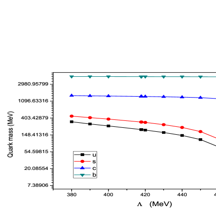
Figure 1: Solutions for constituent quark masses versa the confinement scale value $\Lambda$.

The sharp drop of all quark mass curves in Fig.1 may be shortly explained as follows. Note, two equations in Eqs. (17) mostly differ by meson masses in exponentials along different numerical factors $C_{J}$, $\rho_{J}$ and $\chi_{J}$. They have general solutions $\{m_{ud}\,,\alpha_{s}\}$ not for any $\Lambda$. Suppose, at fixed $\Lambda=\Lambda_{0}$ they are solvable. Then, for finite coupling $\alpha_{s}$ the solution $m_{ud}$ is obviously finite to obey both equations. However, for vanishing $\alpha_{s}\to 0$ the equations take the form

$$1\approx{\alpha_{s}\,C_{J}\over m_{ud}^{2}}\cdot const(\Lambda_{0},M_{J},\rho_{J})$$

and the solution for quark mass behaves $m_{ud}\sim\sqrt{\alpha_{s}}\to 0$. This picture is observed in Fig.1.

By using these quark masses and coupling constant we can estimate other meson masses in dependence on $\Lambda$ and some results are shown in Fig. 2.

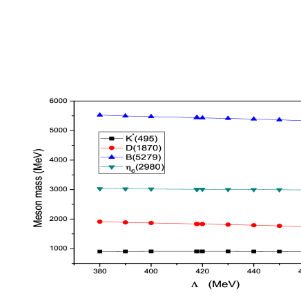
Figure 2: Solutions for some meson masses in dependence on the confinement scale value $\Lambda$.

To fix the value of parameter $\Lambda$ we calculate the weak decay constants $f_{\pi}$ and $f_{K}$ to compare with experimental data. Note, these constants considerably depend on $\Lambda$ (see Fig. 3) that allow us to fix it unambiguously at $\Lambda=416.4$ MeV.

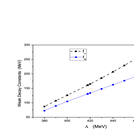
Figure 3: Weak decay constants depending on the confinement scale value $\Lambda$.

The final set of model parameters are fixed as follows:

$$\alpha_{s}=1.5023\,,\qquad\Lambda=416.4{\mbox{\rm~{}MeV}}\,,\qquad m_{ud}=206.9{\mbox{\rm~{}MeV}}\,,$$

$$m_{s}=323.6{\mbox{\rm~{}MeV}}\,,\qquad m_{c}=1453.8{\mbox{\rm~{}MeV}}\,,\qquad m_{b}=4698.9{\mbox{\rm~{}MeV}}\,.$$ (18)

With these parameters we have estimated the pseudoscalar and vector meson masses shown in Table 1 and compared with experimental data [26]. The relative error of our estimate does not exceed $3.5$ percent in the whole range of mass (from 0.14 GeV up to 9.5 GeV).

$J^{PC}=0^{-+}$	$M_{\mathbf{P}}$	$J^{PC}=0^{-+}$	$M_{\mathbf{P}}$	$J^{PC}=1^{--}$	$M_{\mathbf{V}}$	$J^{PC}=1^{--}$	$M_{\mathbf{V}}$
$\pi(138)$	138	$\eta_{c}(2979)$	3012	$\rho(770)$	770	$D^{*}_{s}(2112)$	2078
$K(495)$	495	$B(5279)$	5437	$\omega(782)$	785	$J/\Psi(3097)$	3097
$\eta(547)$	547	$B_{s}(5370)$	5551	$K^{*}(892)$	909	$B^{*}(5325)$	5464
$D(1870)$	1840	$B_{c}(6286)$	6522	$\Phi(1019)$	1022	$\Upsilon(9460)$	9460
$D_{s}(1970)$	1970	$\eta_{b}(9300)$	9434	$D^{*}(2010)$	1942

Table 1: Estimated spectrum of conventional mesons (in units of MeV).

There are mainly two schemes describing $\omega-\Phi$ and $\eta-\eta^{\prime}$ mixings [26]. The octet-singlet scheme uses the mixing angle $\theta$ between states $(u\bar{u}+d\bar{d}-2s\bar{s})/\sqrt{6}$ and $(u\bar{u}+d\bar{d}+s\bar{s})/\sqrt{3}$. We use the quark-flavor based mixing scheme between states $(u\bar{u}+d\bar{d})/\sqrt{2}$ and $s\bar{s}$ with mixing angle $\varphi$. These two schemes are equivalent to each other by $\theta=\varphi-\pi/2+\arctan(1/\sqrt{2})$ when the $SU(3)$ symmetry is perfect. Particularly, for “ideal” vector mixing the angle is $\varphi_{V}^{id}=90^{\circ}$ or $\theta_{V}^{id}=35.3^{\circ}$.

With fixed parameters (18) we calculate a relatively heavy mass $M_{V}(s\bar{s})=1064$ MeV of vector $s\bar{s}$ state. To obtain correct masses of $\omega(782)$ and $\Phi(1019)$ one needs a considerable mixing to the light quark-antiquark state with mixing angle $\varphi_{V}\simeq 73.2^{\circ}$ which differs significantly from the “ideal” value. By using the same parameters (18) we obtain a pseudoscalar $s\bar{s}$ state with mass $M_{P}(s\bar{s})=705$ MeV. We cannot describe the physical mass of $\eta^{\prime}(958)$ by any mixing to the light-quark pair and can only fit the correct mass $M_{P}(\eta)=547$ MeV at angle $\varphi_{P}\simeq 58.5^{\circ}$. Our model fails to describe simultaneously the $\eta-\eta^{\prime}$ mixing. This problem obviously deserves a separate consideration.

Note, the infrared behavior of effective (mass-dependent) QCD coupling $\alpha_{s}$ is not well defined and needs to be more specified [27, 28, 29]. In the region below the $\tau$-lepton mass ($M_{\tau}=1.777$ GeV) the strong-coupling value is expected between $\alpha_{s}(M_{\tau})\approx 0.34$ [26] and the infrared fix point $\alpha_{s}(0)=2.972$ [30]. Our parameter $\alpha_{s}=1.5023$ does not contradict this expectation because it is estimated to fit the $\pi$ meson mass, and so the corresponding energy scale is $\sim 140$ MeV. We keep this value for further calculations.

The weak decay constants of light mesons are well established data and many groups (MILC [31], NPLQCD [32], HPQCD [33], etc.) have these with accuracy at the 2 percent level. Therefore, these values are often used to test any model in QCD. By substituting optimal values of $\{m_{ud},m_{s},\alpha_{s},\Lambda\}$ (18) into (16) we calculate

$$f_{\pi}=128.8{~{}\mbox{\rm MeV}}\,,\qquad f_{K}=157.7{~{}\mbox{\rm MeV}}\,.$$

Our estimates are in agreement with the experimental data [34, 26]:

$$f_{\pi^{-}}^{PDG}=130.4\pm 0.04\pm 0.2\,{\rm MeV}\,,\qquad f_{K^{-}}^{PDG}=155.5\pm 0.2\pm 0.8\pm 0.2\,{\rm MeV}\,.$$ (19)

Our model represents a reasonable framework to describe the conventional mesons, and the parameters are fixed. Below we can consider two-gluon bound states.

4 Glueball Lowest State

Because of the confinement, gluons are not observed, they may only come in bound states called glueballs. Glueballs are the most unusual particles predicted by the QCD but not found experimentally yet [35]. There are predictions expecting non-$q\bar{q}$ scalar objects, like glueballs and multiquark states in the mass range $\sim 1500-1800{\mbox{\rm~{}MeV}}$ [36, 37]. Experimentally the closest scalar resonances to this energy range are the $f_{0}$(1500) and $f_{0}$(1710) [38]. Some references favor the $f_{0}$(1500) as the lightest scalar glueball [39], while others do so for the $f_{0}$(1710) [40, 41]. Recent scalar hadron $f_{0}$(1810) reported by the BES collaboration may also be a glueball candidate [42].

The study of glueballs currently deserves much interest from a theoretical point of view, either within the framework of effective models or lattice QCD. The glueball spectrum has been studied by using effective approaches like the QCD sum rules [43], Coulomb gauge QCD [44], and potential models (e.g., [45, 46]), etc. The potential models consider glueballs as bound states of two or more constituent gluons interacting via a phenomenological potential [45, 47, 48]. It should be noted that potential models have difficulties in reproducing all known lattice QCD data. Different string models are used for describing glueballs [49, 50], including combinations of string and potential approaches [46]. It has been shown that a proper inclusion of the helicity degrees of freedom can improve the compatibility between lattice QCD and potential models [51].

An important theoretical achievement in this field has been the prediction and computation of the glueball spectrum in lattice QCD simulations [52, 53]. Recent lattice calculations, QCD sum rules, ”tube” and constituent glue models predict that the lightest glueball has the quantum numbers of scalar ($J^{PC}=0^{++}$) and tensor ($2^{++}$) states [54]. Gluodynamics has been extensively investigated within quenched lattice QCD simulations and the lightest glueball is found a scalar object with a mass of $\simeq 1.66\pm 0.05$ GeV [55]. A use of much finer isotropic lattices resulted in a value 1.475 GeV [53]. Recently, an improved quenched lattice calculation of the glueball spectrum at the infinite volume and continuum limits based on much larger and finer lattices have been carried out and the scalar glueball mass is calculated to be $1710\pm 50\pm 80$ MeV [56].

Two-gluon bound states are the most studied purely gluonic systems in the literature, because when the spin-orbital interaction is ignored ($\ell=0$), only scalar and tensor states are allowed. Particularly, the lightest glueballs with positive charge parity can be successfully modeled by a two-gluon system in which the constituent gluons are massless helicity-one particles [57].

Below we consider a two-gluon scalar bound state. We isolate the color-singlet term in the bi-gluon current in $Z_{{\cal AA}}$ (4) by using the known relations

$$t^{C}_{ik}\,t^{C}_{jl}={N_{c}^{2}-1\over 2N_{c}^{2}}\delta^{il}\delta^{jk}-{1\over N_{c}}t^{C}_{il}t^{C}_{jk}\,,$$

$$f^{ABE}f^{A^{\prime}B^{\prime}E}={2\over 3}\left(\delta^{AA^{\prime}}\delta^{BB^{\prime}}-\delta^{AB^{\prime}}\delta^{BA^{\prime}}\right)+d^{AA^{\prime}E}d^{BB^{\prime}E}-d^{AB^{\prime}E}d^{BA^{\prime}E}\,.$$

The second-order matrix element containing a color-singlet two-gluon current reads [23]

$$L_{{\cal AA}}= {g^{2}\over 4\cdot 3}\int\!\!\!\int dxdy\left(J^{AA}_{\mu\mu^{\prime}}(x,y)J^{BB}_{\nu\nu^{\prime}}(x,y)-J^{AA}_{\mu\nu^{\prime}}(x,y)J^{BB}_{\nu\mu^{\prime}}(x,y)\right)$$

$$\cdot\left[\delta^{\nu\nu^{\prime}}W_{\mu\mu^{\prime}}(x,y)-\delta^{\mu\nu^{\prime}}W_{\nu\mu^{\prime}}(x,y)-\delta^{\nu\mu^{\prime}}W_{\mu\nu^{\prime}}(x,y)+\delta^{\mu\mu^{\prime}}W_{\nu\nu^{\prime}}(x,y)\right]\,,$$

where

$$J^{BC}_{\mu\nu}(x,y)\doteq{\cal A}^{B}_{\mu}(x){\cal A}^{C}_{\nu}(y)\,,$$

$$W_{\mu\nu}(x,y)\doteq{\partial\over\partial x_{\mu}}{\partial\over\partial y_{\nu}}D(x-y)=\delta^{\mu\nu}\,W(x-y)+\ldots\,,\qquad W(z)={1\over(2\pi)^{2}}\,e^{-z^{2}}\,.$$

This part consists of spin-zero (scalar) and spin-two (tensor) components. Below we consider the scalar component:

$$L_{{\cal AA}}^{S}= {g^{2}\over 3}\int\!\!\!\int dx_{1}dx_{2}J(x_{1},x_{2})W(x_{1}-x_{2})J(x_{1},x_{2})\,,\quad J(x_{1},x_{2})\doteq J^{BB}_{\mu\mu}(x_{1},x_{2})\,.$$

By introducing the relative coordinates ($x_{1}\doteq x+y/2\,,~{}~{}x_{2}\doteq x-y/2$) we rewrite

$$L_{{\cal AA}}^{S}= {g^{2}\over 3}\int\!\!\!\int\!\!dxdy\,J(x,y)W(y)J(x,y)\,.$$ (20)

One can see that the matrix element (20) is similar to (7) by the very construction. By omitting details of intermediate calculations (similar to those represented in the previous section) we rewrite the partition function in terms of auxiliary field $B(x)$ as follows:

$$Z_{{\cal AA}}\rightarrow Z_{G}=\int{\mathcal{D}}B\exp\left\{-{1\over 2}\left(B\,G^{-1}B\right)+L_{I}[B]\right\}\,,$$

where $L_{I}[B]\sim O(B^{3})$ and the BS kernel is

$$G^{-1}(x-y)=\delta(x-y)-{8\,g^{2}\over 3}\Pi(x-y)\,,$$

$$\Pi(z)\doteq\int\!\!\!\int\!\!dtds~{}U_{n}(t)\sqrt{W(t)}~{}D\left({t+s\over 2}+z\right)D\left({t+s\over 2}-z\right)\sqrt{W(s)}~{}U_{n}(s)\,.$$

The hadronization ansatz allows us to identify $B$ with scalar glueball field. To find the glueball mass we should diagonalize the Bethe-Salpeter kernel $\Pi(z)$. The glueball mass $M_{G}$ is defined from equation [24]:

$$1-{8\,g^{2}\over 3}\int\!dz\,e^{izp}~{}\Pi(z)=0\,,\qquad p^{2}=-M_{G}^{2}\,.$$ (21)

For the lightest ground-state scalar glueball choose a Gaussian wave function:

$$U(x)={2c\over\pi}~{}e^{-cx^{2}}\,,\qquad\int\!\!dx\,|U(x)|^{2}=1\,,\qquad c>0\,.$$

Then, we derive (21) as follows:

$$1={\alpha_{s}\over\alpha_{crit}}\exp\left\{{M_{G}^{2}\over 4\Lambda^{2}}\right\}\,,\qquad\alpha_{crit}\doteq{3\pi(3+2\sqrt{2})^{2}\over 4}\,.$$

The final analytic result for the lowest-state glueball mass reads

$$M_{G}=2\Lambda\left[\ln\left({\alpha_{crit}\over\alpha_{s}}\right)\right]^{1/2}\,.$$ (22)

The solution $M_{G}^{2}\geq 0$ exists for any $\alpha_{s}<\alpha_{crit}\approx 80.041$.

Note, the scalar glueball mass depends linearly on the confinement scale $\Lambda$ and the scaled mass $M_{G}/\Lambda$ depends only on coupling $\alpha_{s}$ (see Fig. 4). Particularly, if we take values $\Lambda\sim\Lambda_{QCD}\approx 360$ MeV and $\alpha_{s}\simeq\alpha_{s}(M_{\tau})=0.343$, then we estimate $M_{G}\approx 1710$ MeV.

However, our purpose is to describe simultaneously different sectors of low-energy particle physics. Accordingly, with values $\alpha_{s}=1.5023$ and $\Lambda=416.4{\rm\,MeV}$ determined by fitting the meson masses and weak decay constants, we calculate the scalar glueball mass as follows:

$$M_{G}=1661{\mbox{\rm~{}MeV}}\,.$$ (23)

Our estimate (23) is in reasonable agreement with other predictions expecting the lightest glueball located in the scalar channel in the mass range $\sim 1500-1800{\rm~{}MeV}$ [36, 43, 53, 58]. The often referred quenched QCD calculations predict $1750\pm 50\pm 80{\mbox{\rm~{}MeV}}$ for the mass of the lightest glueball [52]. The recent quenched lattice estimate with improved lattice spacing favors a scalar glueball mass $M_{G}=1710\pm 50\pm 58{\rm~{}MeV}$ [56].

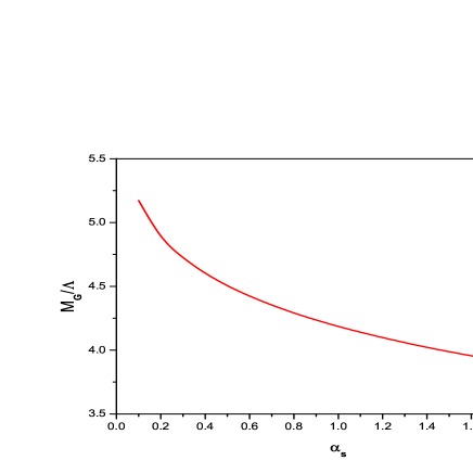
Figure 4: Evolution of the lowest-state glueball mass scaled to $\Lambda$ with the coupling $\alpha_{s}$.

Another important property of the scalar glueball is its size, the “radius” which should depend somehow on the glueball mass. We estimate the glueball size by using the “effective potential” $W(y)$ (20) connecting two scalar gluon currents. The glueball radius may be roughly estimated as follows

$$r_{G}\sim\sqrt{{\int\!d^{4}x~{}x^{2}~{}W(x)\over\int\!d^{4}x~{}W(x)}}={\sqrt{2}\over\Lambda}\approx{1\over 295~{}\mbox{\rm MeV}}\approx 0.67~{}\mbox{\rm fm}\,.$$ (24)

This means that the dominant forces responsible for binding gluons must be provided by medium-sized vacuum fluctuations of correlation length $\sim 0.7\,\mbox{\rm fm}$. Consequently, typical energy-momentum transfers inside a scalar glueball occur at the QCD scale $\sim 360$ MeV, rather than at the chiral symmetry breaking scale $\Lambda_{\chi}\sim 1$ GeV (or, $\sim 5\,{\rm fm}$).

From (22) and (24) we deduce that

$$r_{G}\cdot M_{G}=2\sqrt{2}\left[\ln\left({\alpha_{crit}\over\alpha_{s}}\right)\right]^{1/2}\approx 5.64\,.$$

This value may be compared with the prediction ($r_{G}\cdot M_{G}=4.16\pm 0.15$) of quenched QCD calculations [52, 56]. A study of the glueball properties at finite temperature using SU(3) lattice QCD at the quenched level with the anisotropic lattice imposes restrictions on the glueball parameters at zero temperature: $0.37\,{\rm fm}<r_{G}<0.57\,{\rm fm}$ and $M_{G}\simeq 1.49\,{\rm GeV}$ [59]. The nonprincipal differences of quenched lattice QCD data from our estimates may be explained by the presence of quarks (our parameters have been fixed by fitting two-quark bound states) in our model.

A method of analysis of correlation functions in QCD is to calculate the corresponding condensates. The value of the correlation function dictates the values of the condensates. We calculate the lowest nonvanishing gluon condensate in the leading-order (ladder) approximation:

$$g^{2}Tr\left\langle F_{\mu\nu}^{A}F^{\mu\nu}_{A}\right\rangle=8N_{c}\pi\alpha_{s}\Lambda^{4}\int\!\!d^{4}z\,W(z)=6\pi\alpha_{s}\Lambda^{4}\approx 0.8~{}GeV^{4}$$

which is the same order of magnitude with the reference value [60]

$$g^{2}Tr\left\langle G_{\mu\nu}G^{\mu\nu}\right\rangle\approx 0.5~{}GeV^{4}\,.$$

In conclusion, the suggested model in its simple form is far from real QCD. However, our aim is to demonstrate that global properties of the lowest glueball state and conventional mesons may be explained in a simple way in the framework of a simple relativistic quantum-field model of quark-gluon interaction based on analytic confinement. Our guess about the symmetry structure of the quark-gluon interaction in the confinement region has been tested and the use of simple forms of propagators has resulted in quantitatively reasonable estimates in different sectors of the low-energy particle physics. The consideration can be extended to other problems in hadron physics.

The author thanks G.V. Efimov, E. Klempt and V. Mathiew for valuable remarks and useful suggestions.

References

- [1] V. A. Miransky, ’Dynamical Symmetry Breaking in Quantum Field Theories’ (Word Scientific, 1993).
- [2] C. S. Fischer and R. Alkofer, hep-ph/0301094.
- [3] H. Leutwyler, Phys. Lett., 96B (1980) 154; Nucl. Phys. B179, 129 (1981).
- [4] M. Sting, Phys. Rev. D29, 2105 (1984).
- [5] T. C. Kraan and P. van Baal, Nucl. Phys. B533, 627 (1998).
- [6] R.Alkofer and J. Greensite, J. Phys. G34, s3 (2007).
- [7] F. Lenz, J. W. Negele and M. Thies, Phys. Rev. D69, 074009 (2004).
- [8] E. Elizalde and J.Soto, Nucl. Phys. B260, 136 (1985).
- [9] G.V. Efimov and S.N. Nedelko, Phys. Rev. D51, 176 (1995); Phys. Rev. D54, 4483 (1996); Ya.V. Burdanov and G.V.Efimov, Phys. Rev. D64, 014001 (2001).
- [10] M. Baldicchi and G.M. Prospri, arXiv:hep-ph/0310213 (2003).
- [11] J. Gasser and H. Leutwyler, Ann. Phys. 158, 142 (1984); Nucl. Phys. B250, 465 (1985).
- [12] M. A. Shifman, A. I. Vainshtein and V. I. Zakharov, Nucl. Phys. B147, 385 (1979).
- [13] M. Neubert, Phys. Rep. 245, 259 (1994).
- [14] R. Gupta, hep-lat/9807028.
- [15] C. D. Roberts, arXiv:0802.0217 [nucl-th]; C. D. Roberts and S. M. Schmidt, Prog. Part. Nucl. Phys. 45, s1 (2000).
- [16] E.E. Salpeter and H.A. Bethe, Phys. Rev. 84, 1232 (1951).
- [17] C. D. Roberts and A. G. Williams, Prog. Part. Nucl. Phys. 33, 477 (1994).
- [18] G.V. Efimov and G. Ganbold, Phys. Rev. D65, 054012 (2002).
- [19] G. Ganbold, AIP Conf. Proc. 717, 285 (2004); ibid 796, 127 (2005).
- [20] G. Ganbold, arXiv:hep-ph/0512287 (2005).
- [21] G. Ganbold, arXiv:hep-ph/0610399 (2006).
- [22] G. Ganbold, arXiv:hep-ph/0611277 (2006).
- [23] G. Ganbold, EConf C070910, 228 (2007).
- [24] G. Ganbold, PoS Confinement8, 085 (2008).
- [25] T. Feldman, Int. J. Mod. Phys. A15, 159 (2000).
- [26] Review of Particle Physics, C. Amsler et al., Phys. Lett. B667, 1 (2008).
- [27] D.V. Shirkov, Theor. Math. Phys. 132, 1309 (2002).
- [28] A.V. Nesterenko, Int. J. M. Phys. A18, 5475 (2003).
- [29] O. Kaszmarek and F. Zantow, Phys. Rev. D71, 114510 (2005).
- [30] C.S. Fischer and D. Zwanziger, Phys. Rev. D 72, 054005 (2005).
- [31] C. Bernard et al. [MILC Collaboration], PoS LAT2007, 090 (2007).
- [32] S. R. Beane et al. [NPQCD Collaboration], Phys. Rev. D75, 094501 (2007).
- [33] E. Follana et al. [HPQCD Collaboration], arXiv:0706.1726 [hep-lat] (2007).
- [34] C. Bernard et al., PoS LAT2005, 025 (2005).
- [35] E. Klempt and A. Zaitsev, Phys. Rep. 454, 1 (2007).
- [36] C. Amsler, N.A. Tornqvist, Phys. Rep. 389, 61 (2004).
- [37] D.V. Bugg, Phys. Rep. 397, 257 (2004).
- [38] W.-M. Yao et al., J. Phys. G33, 1 (2006).
- [39] D.V. Bugg, M.J. Peardon and B.S. Zou, Phys. Lett. B486, 49 (2000).
- [40] J. Sexton, A. Vaccarino and D. Weingarten, Phys. Rev. Lett. 75, 4563 (1995).
- [41] M.S. Chanowitz, Phys. Rev. Lett. 98, 149104 (2007).
- [42] M. Ablikim, et al. [BES Collaboration], Phys. Rev. Lett. 96, 162002 (2006).
- [43] S. Narison, Nucl. Phys. B509 (1998) 312; Nucl. Phys. A675, 54 (2000).
- [44] A.P. Szczepaniak and E.S. Swanson, Phys. Lett. B577, 61 (2003).
- [45] J.M. Cornwall and A. Soni, Phys. Lett. B120, 431 (1983).
- [46] F. Brau, C. Semay, and B. Silvestre-Brac, Phys. Rev. D70, 014017 (2004).
- [47] A.B. Kaidalov and Yu.A. Simonov, Phys. Lett. B636, 101 (2006).
- [48] V. Mathieu, C. Semay, and B. Silvestre-Brac, Phys. Rev. D74, 054002 (2006).
- [49] K. Yamada, S. Ishida, J. Otokozawa, N. Honzawa, Prog. Theor. Phys. 97, 813 (1997).
- [50] L.D. Soloviev, Theor. Math. Phys. 126, 203 (2001).
- [51] V. Mathieu, C. Semay, and F. Brau, Eur. Phys. J. A27, 225 (2006).
- [52] C.J. Morningstar and M. Peardon, Phys. Rev. D60, 034509 (1999).
- [53] H.B. Meyer and M.J. Teper, Phys. Lett. B605, 344 (2005).
- [54] W. Ochs, arXiv:hep-ph/0609207 (2006).
- [55] A. Vaccarino and D. Weingarten, Phys.Rev. D60, 114501 (1999).
- [56] Y. Chen et. al., Phys. Rev. D73, 014516 (2006).
- [57] V. Mathieu, F. Buisseret, and C. Semay, Phys. Rev. D77, 114022 (2008).
- [58] G.S. Bali, arXiv:hep-ph/0110254 (2001).
- [59] N. Ishii, H. Suganuma and H. Matsufuru, arXiv:hep-lat/0106004 (2001).
- [60] M.A. Shifman, University Minnesota, TRI-MINN-98/10-T; UMN-TH-1622-98 (1998).