Renormalization-group investigation of the $S=1$ random antiferromagnetic Heisenberg chain

Abstract

We introduce variants of the Ma-Dasgupta renormalization-group (RG) approach for random quantum spin chains, in which the energy-scale is reduced by decimation built on either perturbative or non-perturbative principles. In one non-perturbative version of the method, we require the exact invariance of the lowest gaps, while in a second class of perturbative Ma-Dasgupta techniques, different decimation rules are utilized. For the $S=1$ random antiferromagnetic Heisenberg chain, both type of methods provide the same type of disorder dependent phase diagram, which is in agreement with density-matrix renormalization-group (DMRG) calculations and previous studies.

PACS Nos.: 05.50.+q, 64.60.Ak, 68.35.Rh

1 Introduction

In recent years intensive research work has explored some curious properties of antiferromagnetic Heisenberg chains.[1, 2, 3, 4, 5, 6] The features of the pure systems are well-known after Haldane’s seminal work:[1] half-integer $S$ and integer $S$ chain show distinct behavior; gapless spectra, quasi-long-range order and gapped spectra, hidden topological order characterize them, respectively. In $S=1/2$ chain, Ma and Dasgupta introduced a RG technique,[4, 6] with which it was possible to point out that any small amount of disorder triggers the random-singlet phase (RSP) where spins in arbitrarily large distance are coupled in singlets. In $S=1$ chain,[7, 8, 9, 10, 11, 12, 13, 14, 15] only sufficiently large disorder is able to change the pure system properties.

The $S=1$ random antiferromagnetic Heisenberg chain (RAHC) was studied numerically with density-matrix renormalization-group (DMRG) [11, 21, 22, 23, 24, 25] and quantum Monte Carlo (QMC) technique,[13, 14, 15, 26] a considerable part of the findings was contributed by extended versions[7, 8, 9, 10] of the Ma-Dasgupta RG method that is based on a perturbative decimation step, which fails for higher-S RAHC for weak disorder, but asymptotically correct for strong disorder, therefore, it is known as strong-disorder RG (SDRG). The SDRG method has been applied in chains,[27, 28] ladders,[29] in two-, and three-dimensional systems,[30] for a review by Iglói and Monthus, see Ref. Ferenc.

In this paper, a non-perturbative RG technique is presented, which is inspired by the SDRG method[4, 5] and in which the lowest gaps play the central role, therefore it is termed as gap RG (GRG). The original SDRG is investigated: a simple argument is presented and justified, by using local and global aspects of disorder, to explain the success of the SDRG, which holds true in higher-$S$ chains.[33]

The structure of the paper is the following: in Section 2, the model and the failure of the SDRG decimation are described. The results of the GRG and the disorder-induced phases are described in Section 3. Different SDRG methods, the interpretation and justification of their correctness, are detailed in Section 4. The results are summarized and compared to earlier findings, in Section 5.

2 The random antiferromagnetic Heisenberg chain and the strong-disorder renormalization

We investigate the $S=1$ RAHC with Hamiltonian

$$H=\sum_{i=1}^{L-1}J_{i}\vec{S}_{i}\cdot\vec{S}_{i+1}.$$ (1)

The $J_{i}>0$ couplings follow a random distribution, the power-law distribution

$$p_{\delta}(J)=\delta^{-1}J^{-1+1/\delta}\ \ \ \ \ {\rm for}\ 0\leq J\leq 1\ \$$ (2)

where the $\delta$ parameter tunes the strength of disorder as $\delta^{2}=\rm var[\ln\it J]$; $\delta=0$, $\delta=1.0$, and $\delta\to\infty$ denote pure, uniform, and infinite randomness, respectively. This system has a relevance in solid state physics,[34] in quantum computations,[35] and serves as a testing ground for developing novel methods and theories.[16, 36]

In a given RAHC, the SDRG method eliminates iteratively the largest coupling with its four neighboring spins and replaces it by two spins with a new coupling, see Fig. 1, determined by perturbation theory for general $S$ as

Figure 1: The four-spin system with the largest coupling parameter $\Omega$ replaced by a two-spin system with coupling constant given in Eq.(3), in a usual SDRG decimation, or such $J^{\prime}$ which involves an identical first gap as that of the original four-spin subchains, in a GRG decimation.

$$J^{\prime}=\frac{2}{3}\frac{S(S+1)J_{1}J_{3}}{\Omega}\;.$$ (3)

The method works in $S=1/2$ RAHC where the new coupling $J^{\prime}=J_{1}J_{3}/2\Omega$ is smaller than any of the eliminated ones. For higher-$S$ RAHC the $(2/3)S(S+1)>1$, the new coupling can be larger than the decimated one: the method fails for weak disorder. In order to circumvent this problem, novel RG schemes were initiated[7, 8, 9, 10] that use a set of decimation steps and deal with a mixture chain of $S=1/2$ and $S=1$ spins. These RG schemes predict a transition from the pure system behavior to the RSP, which was tested with DMRG[11] and QMC.[26, 14] Saguia et al.[12] use a different strategy to tackle the problem, they keep the original SDRG decimation, if it works correctly, and replace it with a two-step perturbative decimation, if it fails. The method yields three phases: gapped/gapless Haldane phase (or nonsingular/singular Griffiths phases), and RSP.

3 Gap renormalization-group method

We briefly describe a non-perturbative RG method that has a similar iterative strategy as the SDRG: it eliminates the largest couplings, but the decimation rule is different, the new coupling is determined with the condition that the first gap is invariant, see Fig. 1. The system properties can be drawn from the first gap distribution and by analyzing the RG flows. The GRG works in higher-$S$ RAHC and in $S=1/2$ chain in its original form.[33] Preliminary results of GRG were published in Ref.Lajko2. In the following, more detailed investigations are presented.

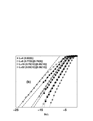
Figure 2: Integrated probability distribution of the first gaps at $\delta=0.5$ (a) and at $\delta=1.0$ (b) disorder. In terms of the slopes of the low-gap region, the agreement is obvious, although the GRG data (empty symbols) are shifted toward the low-gap region. DMRG data (filled symbols) are available up to $L=32$, the GRG data are plotted also up to this length. The estimated slopes are indicated in the legends (i.e., {DMRG slopes} and [GRG slopes]) and plotted with dashed lines.

3.1 The disorder-induced phases and finite-size corrections

We have investigated the $S=1$ RAHC by using the GRG technique and DMRG[21, 22, 23, 24, 25] method in parallel. We eliminated iteratively $L-4$ spins from the original $L$ by using the GRG method, the new couplings were always smaller than the eliminated ones, and the final four-spin system is diagonalized by the Lánczos method. On the other hand, genuine first gaps are calculated by using DMRG method.

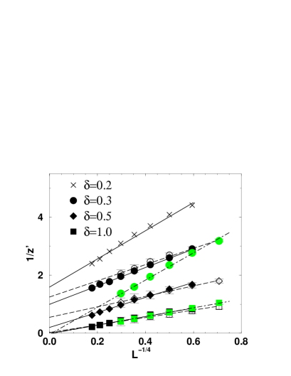
Figure 3: The $1/z^{\prime}$ exponent. Empty symbols (dashed lines) denote the GRG data (fitted straight lines). Full symbols (solid lines) denote the SDRG data. Opaque symbols (dot-dashed lines) denote the XX chain data. Error bars, if not indicated, are smaller than the symbols.

The basis number in DMRG calculations was so large (maximum $180$) that it did not influence the probability distribution.

The comparison was made for different strength of disorder, always a very good agreement was found between the original gap integrated probability distribution and the GRG data in the sense that the slopes of the low-gap tail from GRG and DMRG are the same, see in Fig. 2. In fact, this is the first time that RG results of $S=1$ RAHC are faced to genuine probability distributions.

The dynamical exponent $z$ can be determined via the scaling of the first gap probability densities (and integrated probability densities) in the low-gap region:

$$P(\ln\Delta)\sim\Delta^{1/z^{\prime}},$$ (4)

where $z^{\prime}$ is identical to the dynamical exponent $z$, if $z^{\prime}>1$, otherwise $z=1$. From the low-gap tail of the integrated probability distributions the slopes ($1/z^{\prime}$) in the log-log plot are extracted for different sizes and $\delta$ parameter, Fig. 3. In this parameter region, the following relation is conjectured and utilized in the figure

$$\frac{1}{z^{\prime}(\delta,L)}\approx\frac{1}{z^{\prime}(\delta,\infty)}+A(\delta)L^{-1/4}.$$ (5)

$1/z^{\prime}(\delta,\infty)$ helps to identify the phase diagram of the $S=1$ RAHC. At very weak disorder, up to $\delta_{1}=0.4(15)$, $z^{\prime}(\delta,\infty)$ is smaller than $1$ indicating the nonsingular Griffiths phase.[32] At intermediate disorder $0.4<\delta<1.0$, $z^{\prime}(\delta,\infty)$ has still finite value, singular Griffiths phase, while above $\delta_{c}=1.00(15)$ we have found $z^{\prime}=\infty$ in the large-$L$ limit indicating the appearance of RSP.

Figure 4: The phase diagram. $\delta=0$ denotes the pure system, $\delta_{1}$ the phase boundary between the nonsingular and singular Griffiths phases, $\delta_{c}$ the phase boundary between Griffiths phase and RSP.

We have performed SDRG also on XX chains and analyzed the gap distributions in the same size region. The XX chain is chosen because its decimation rule,[37] with 1 prefactor in Eq.(3), is the closest to the decimation rule of $S=1$ RAHC, with prefactor $4/3$. The slopes, extracted from the XX chain at $\delta=0.3$ and $\delta=1.0$ and plotted in Fig. 3, scale with effective exponent $-1/4$ and predict disappearing $1/z^{\prime}$, as it is expected,[6] and thus justify the assumption that these system sizes provide physically conclusive results in the large-$L$ limit.

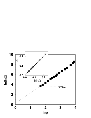
Figure 5: Analysis of the GRG flow at $\delta=1.0$. The $\psi$ exponent from the density of active spins is identified from the slope as $1/2$. Inset: The $\alpha$ parameter can be identified as $\alpha=-1/\ln\Omega$.

3.2 Gap renormalization flow in the RSP

In RSP during the RG treatment of a certain random chain, the ratio of the remaining spins that are not decimated out follows the scaling law[6]

$$\rho=\frac{1}{L}=\frac{1}{|\ln\Omega|^{1/\psi}}.$$ (6)

This relation describes the connection between the characteristic length scale of the system $L$ and the energy scale $\Omega$ via the $\psi=1/2$ exponent, a characteristic relation of RSP. The GRG method is applied on very large system sizes, $20$ million spins, results are plotted in Fig.5. The slope of the double logarithmic plot reveals the presence of RSP in the system at $\delta=1.0$ disorder.

The following aim is to show out that the scaling of the coupling distribution under GRG procedure follows the expected RSP behavior:[6]

$$P_{\Omega}(J)=\frac{\alpha}{\Omega}\left(\frac{\Omega}{J}\right)^{1-\alpha}$$ (7)

with $\alpha=-1/\ln\Omega$. Actually, the above type of scaling is found at $\delta=1.0$, see the inset in Fig.5 where $\alpha$, determined from the slope of the coupling distribution, is depicted as a function of $-1/\ln\Omega$. Both quantities, the coupling distribution and the fraction of undecimated spins follow the scaling that is characteristic of the RSP.

4 Results of the SDRG

In this section, different aspects of SDRG method are analyzed and discussed. Firstly, proper interpretation of the strong-disorder limit is presented that explains the reliability of SDRG method. Secondly, the scaling relations and the corresponding finite-size corrections of SDRG data are discussed. Finally, an unusual representation of the SDRG flows is established that has a very high accuracy.

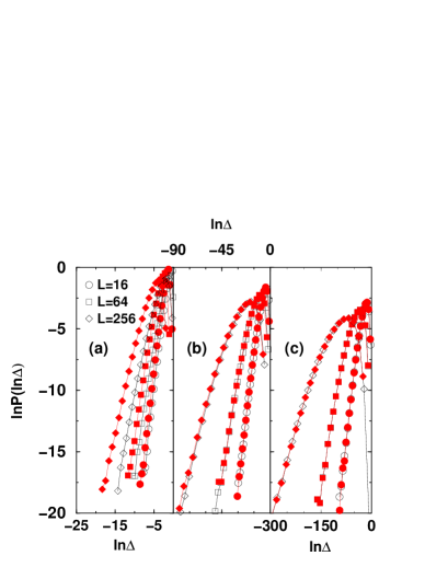
Figure 6: (Color online) The gap distributions generated by the original SDRG (empty symbols) and the modified SDRG (filled symbols) for $\delta=0.3,1.0,3.0$ disorder in (a), (b), and (c), respectively.

4.1 The low-gap region of the probability distributions

One has to clearly distinguish two different kinds of appearance of disorder: global and local appearances. On the one hand, the global disorder describes the statistical ensemble of couplings in the chains and it can be parameterized, in this work, with the $\delta$ parameter of the power-law distribution. On the other hand, the local disorder or subchain disorder characterizes only one particular four-spin subchain and it can be parameterized, for instance, with the value $\max(J_{1},J_{3})/\Omega$.

The SDRG can be correct in the proper strong-disorder limit: if the subchain disorder is strong everywhere in a chain that is already a sufficient condition. In certain chains the strong subchain or local disorder can be present generally at arbitrary location in the chain with some small probability that itself depends on the global disorder that describes the statistical ensemble of the couplings. These probably rare chains provide the smallest gaps to the gap distributions since in these chains repeatedly very small new couplings are replaced in the consecutive decimations resulting the smallest final couplings and gaps. Consequently, the low-gap regime of the results can be correct, in RG sense, at any given strength of global disorder, as they come via the correct decimation steps from those rare chains in which the subchain disorder is strong everywhere. This interpretation of the low-gap region is in accordance with the well-established scenario of rare region effects.[38, 39]

4.2 Comparison of the original and the modified SDRG

In order to make this feature more transparent, we present a systematic investigation and comparison of SDRG and modified SDRG results in the low-gap region of the probability distributions. The original SDRG method is straightforward, the modified SDRG applies the same decimation rule except in those cases in which the new coupling $J^{\prime}$ is larger than at least one of $J_{1}$ and $J_{3}$. In those decimation steps $cJ^{\prime}$, with $c\leq 1/[(2/3)S(S+1))]=3/4$, is used as a new coupling ensuring always smaller new coupling than the decimated ones. The two schemes are almost identical, the only difference is factor $c$ if the perturbative decimation fails.

This modified version of SDRG has a similar scenario as the RG method applied in Ref. Con. However, the modification is very simple here, just a rescaling of the coupling given by the original rule, whereas a two-step degenerate perturbative decimation isis applied in Ref.Con. Nevertheless, the heuristic argument used here to explain the success of SDRG applies also for the modified version SDRG in Ref. Con.

These two RG schemes, the original SDRG and the modified one have been applied to generate the gap distribution for several system sizes and strength of disorder. The two types of gap distributions are plotted in Fig. 6; the slopes of the low-gap regions are identical for fixed sizes and strengths of global disorder. The plotted results were generated with $c=2/3$ in the modified decimation steps, but several other values provided identical slopes in the low-gap region.

The slope of the low-gap region is apparently independent of those decimation steps where the original decimation rule fails in perturbative sense. The modified RG steps, by generating smaller coupling than the original one, shift the corresponding low-gap distributions towards the lower gaps, but the structure of this regime remains the same as in the original case. A similar relation of the GRG and DMRG results is observed in Fig. 2. For longer chains that involve more decimation steps, the shift between the two gap distributions is more enhanced, see Fig. 6. For sufficiently strong global disorder the modified decimation steps practically do not make change on the structure of the gap distributions, at least for smaller chain sizes, see Fig. 6(b) and (c) for $\delta=1.0$ and $\delta=3.0$ disorder, respectively.

4.3 Disorder-induced phase diagram

The original SDRG results were carefully analyzed and the estimates of $1/z^{\prime}$ were extracted for different system sizes and plotted in Fig.3 as a function of $L{{}^{-1/4}}$. These numerical values are in agreement with the results of GRG method. The estimates for the phase boundaries $\delta_{1}=0.29(6)$, $\delta_{c}=1.0(1)$ are in rather good agreement with other studies.

One has to notice, the finite-size corrections are smaller in the Griffiths phase than in the RSP, in terms of the dynamical exponent $z$, and are weakening deeper into Griffiths phase. The SDRG results are more reliable than the GRG results. Firstly, more random chains are averaged for SDRG, at least 80 million, and only 2 million for the GRG. Secondly, larger systems are analyzed for the SDRG ($L=1024$ and only $L=128$ for GRG). Even larger system sizes were tested, however for those sizes the convergence in the low-gap region was not satisfactory although intensive computations were performed on a Beowulf Linux cluster in order to have accurate gap distributions from GRG, SDRG, DMRG methods.

Figure 7: (a) Gap distribution generated by the original SD RG method at $\delta=0.5$. (b) Scaling collapse assuming Griffiths phase with scaling relation in Eq.(9) and $z=5.0$.

4.4 Scaling of the SDRG data

In the following, the scaling of the SDRG results in the $S=1$ RAHC are tested by the expected scaling laws[6] in the Griffiths phase and in the RSP that are shown out exactly, for instance, in the random transverse-field Ising spin chain, in the $S=1/2$ RAHC or in the random XX chain. In the Griffiths phase, the energy scale $\Omega$ is continously reducing during the RG, and the couplings follow the distribution

$$P(J,\Omega)dJ=\frac{1}{z}\left(\frac{J}{\Omega}\right)^{-1+1/z}\frac{dJ}{\Omega}.$$ (8)

Due to the relation of energy scale and the length of the system ( $\Omega\sim L^{-z}$) and by assuming that the RG process leaves the $z$ exponent unaltered, one can conclude easily Eq.(4) and the scaling law

$$P_{L}(\ln\Delta)=P(\ln(\Delta L^{z})).$$ (9)

In the RSP, where $z$ is infinity, one can set formally $z=-\ln\Delta\sim L^{\psi}$, Eq.(6) transforms into Eq.(7), and the corresponding scaling relation is

$$P_{L}(\ln\Delta)=L^{-\psi}P(\ln(\Delta)/L^{\psi}))$$ (10)

with $\psi=1/2$. These scaling laws were successfully utilized, for instance, in the random XX spin chains,[46] in the $S=1/2$ RAHC[41] and also in higher-dimensional systems,[30] but were never tested in the $S=1$ RAHC due to the known reasons.

On the one hand, these scaling laws assume that the investigated sizes are free of finite-size corrections. If this condition is not accomplished, and it is not accomplished in the $S=1$ RAHC, one can expect the appearance of finite-size corrections in addition to the above detailed leading behavior. On the other hand, Eq.(8) assumes the monotoniicc decrease of the energy scale $\Omega$ that is surely not rigorously true during the original SDRG in the $S=1$ RAHC, therefore Eq.(8) is surely not accurately true. However, Eq.(8) can be true in a looser sense, i.e., its consequences, Eq.(4), Eq.(6), Eq.(9) and Eq.(10), can be true since the extraction of these relations does not assume the rigorous accurateness of Eq.(8). The probability distribution in the low-gap region follows the expected behavior, Eq.(4), as shown in the earlier subsection. The scaling behavior in the Griffiths phase, Eq.(9), and in the RSP, Eq.(10), are investigated in the following paragraphs.

The SDRG gap distributions are plotted in Fig.7 for $\delta=0.5$ disorder. One can notice a systematic broadening in the distributions and systematic change in the slopes of the low-gap region with increasing systems sizes, which can be considered as a result of finite-size corrections. The presence of finite-size corrections is evident also from Fig. 3, where the estimated slopes are plotted. Due to these finite-size corrections the expected scaling collapse is not perfect, see Fig.7(b). It is to be emphasized that the values of the $z$ exponent in the scaling collapse are taken from the large-$L$ estimates in Fig.3 and they are not optimized for the scaling collapse itself. In order to have even better scaling collapse by using the same large-$L$ limit estimates of $z$ or to see a satisfying fit with an analytically estimated gap distributions,[40] one should study drastically larger systems sizes.

Figure 8: (a) Gap distribution generated by the original SDRG method at $\delta=1.0$. (b) The scaling collapse assuming RSP and the scaling relation in Eq.(10) with $\psi=1/2$, and with $\psi=1/3$ (c).

The scaling collapse is tested also in the RSP. The gap distributions of the original SDRG are clearly broadening with increasing system sizes, Fig. 8(a), the changes in the slopes are more pronounced than in Fig. 7, indicating broadening without limit and the presence of RSP. The scaling collapse is not perfect for the investigated sizes, although there is apparently a crossover phenomenon present: for larger sizes the collapse is almost perfect, see Fig.8(b).

In addition, the scaling collapse is examined with and exponent $\psi=1/3$ as this value of exponent was theoretically predicted in Ref. Monthus,Monthusa and numerically found in Ref. Lajko2 at the critical point, see Fig.8(c). It can be argued that the scaling collapse is far better with $\psi=1/2$ than with $\psi=1/3$. For $\psi=1/2$, the collapse is almost perfect in the large-gap region and there is a systematic improvement for larger sizes in the low-gap region. Very recently, $\psi=1/3$ was found with scaling investigation of DMRG results[32] at the same disorder for relatively small system sizes. The results presented here in Fig.8 imply that the $1/3$ value of exponent is only an effective value due to a crossover phenomenon. Since there is a uncertainty regarding the value of $\delta_{c}$, the scaling collapse of RSP was investigated at several different strength of disorder in the $\delta\sim 0.7-1.5$ region. In this region, the $1/2$ exponent gives always better scaling collapse than the $1/3$ exponent.

We think that the presence of crossover phenomena, discussed here in detail, associated with changing finite-size corrections is the explanation why the $S=1$ RAHC represents a very challenging problem often leading to controversial results regarding the location of phase boundaries, see Section 7.5. in Ref. Ferenc or Table II in Ref. Lajko2. This phenomenon is reported in detail in the $S=1/2$ RAHC in Ref. Rieger,Riegera,Riegerb, but also known in other quantum spin chains.[25]

To summarize the scaling collapse investigation, scaling collapse considerations should be carefully inspected as there are affected by finite-size effect, while the finite-size corrections allow a rather accurate estimates of different phases in terms of the slopes of the distributions in the low-gap regions.

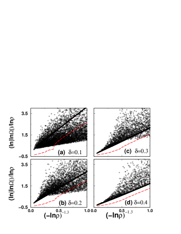
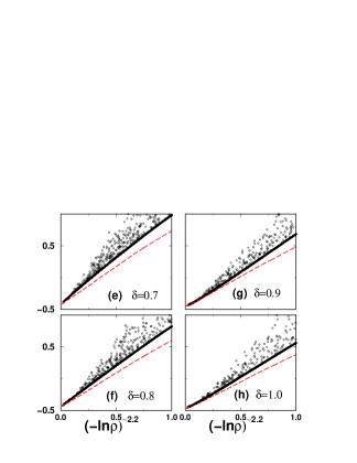
Figure 9: (Color online) Symbols denote the largest coupling applying the original SDRG method. Thick (red) staggered lines denote the same when the modified SDRG is used. Renormalization flows are depicted for $\delta=0.1,0.2,0.3,0.4,0.7,0.8,0.9,1.0$ in Fig. (a)-(h), respectively. The $-1.3$ and $-2.2$ exponents in the label of the horizontal axis are determined in a fitting procedure.

4.5 Analysis of SDRG flows and the $\psi$ exponent

SDRG and modified SDRG results were confronted also to relations in Eq.(6) and (7) with the same conclusion as it is plotted in Fig.5 at $\delta=1.0$ disorder, but unfortunately also in a region below this strength of disorder due to considerable errors. This indicates that probably other representations of RG flow are more proper to describe the phase diagram and the appearance of the RSP. It is found that the best quantity to be investigated is $\ln(|\ln\Omega|)/\ln\rho$ as a function of $\ln\rho$. From Eq. (6), it is evident that assuming the presence of RSP this product should tend to $-0.5$ in the small-$\rho$ limit.

The results of this investigation are plotted in Fig.9 for both the original and modified SDRG cases. The data are independent of the original length of the chain, which is 1 million in each plotted case, they are practically free of finite-size corrections and thus allow a very precise estimate on $\psi$.

For weak disorder, very large fluctuations dominate the data, Fig.9, which gradually decrease for stronger disorder. Around $\delta=0.2-0.4$ an envelope curve appears below the fluctuating data points that allows a straight line fit for small-$\rho$ estimate. With increasing disorder the small-$\rho$ estimates gradually reach the $-0.5$ value, at $\delta=\delta_{c}$, and remains there for stronger disorder. This representation provides a very accurate prediction: RSP appears at $\delta_{c}=1.00(3)$ disorder. Notice that the small-$\rho$ estimates gradually decrease to $-0.5$ and then with further increase of the strength of disorder they remain there, indicating clearly that the phase transition point is at $\delta_{c}=1.00(3)$ where $\psi_{c}=0.50(1)$ but $\psi=0.5$ also deep in the RSP.

5 Summary of the results and comparison to earlier findings

In this paper, a non-perturbative GRG scheme and different variants of the perturbative SDRG method give a coherent picture about the disorder-induced phase diagram of $S=1$ RAHC.

The GRG method provides an accountable phase diagram: for weak disorder, the system is in a Griffiths phase with a disorder-dependent dynamical exponent; for stronger disorder the systems reaches the RSP, at $\delta=\delta_{c}$, where the dynamical exponent is infinity. The Griffiths phase can be further divided, at $\delta=\delta_{1}$, into nonsingular and singular phases. GRG provides reasonable estimates on the phase boundaries by applying finite-size scaling analysis, see Fig.3, $\delta_{1}=0.40(15)$ and $\delta_{c}=1.00(15)$. From a theoretical point of view, the GRG scheme is well-established; from a numerical point of view, the data from GRG technique is well-justified.

The original and modified SDRG properly describe, in contrast to the earlier expectation, the features of the system and provide a high accuracy for the phase boundaries in the large-$L$ limit: $\delta_{1}=0.29(6)$ and $\delta_{c}=1.01(3)$, in quantitative agreement with the latest works. The exponent $\psi$ is shown out with different approaches and consistently found to be $0.5$ in the RSP and in the critical point.

The findings of this work are at least in qualitative agreement with all of the earlier studies. This agreement can be considered, beyond the direct DMRG test at smaller sizes, as indirect test of the SDRG method in the asymptotic regime.

Good quantitative agreement can be observed with the latest numerical investigations. The $\delta_{1}$ and $\delta_{c}$ phase boundaries, determined in this work, are very close to the values in Ref. Con,Todoa,Todob,Lajko2. Hida’s early but hidden estimate of $\delta_{c}$, see Fig.3 in Ref. Hida, is also close to $1.01(3)$ that is the best estimate for $\delta_{c}$ in this work. The phase boundary $\delta_{1}=0.29(6)$, deep in the Griffiths phase, well coincides with independent estimates: $\delta_{1}=0.23$ (the relation of the power-law and box distribution is detailed in Ref. Rieger) in Ref. Con and $\delta_{1}=0.45$ in Ref. Lajko2.

There is a group of studies that successfully describe the phases in the $S=1$ RAHC by decomposing the $S=1$ spins into $S=1/2$ spins in an SDRG scheme. The success of these well-established methods is not questioned by the success of the original SDRG method; however, with these earlier works only a qualitative agreement is found, because these works contribute only qualitative description of two phases RSP and a Griffiths phase[18] or they predict rather distinct phase boundaries: $\delta_{c}\sim 0.77$ is found in Ref. Monthus,Monthusa and $\delta_{c}\sim 1.5$ in Ref. Yanga.

One of the earliest extended SDRG study[7, 8] predicts distinct $\psi$ exponent in the critical point ($\psi_{c}=1/3$) and in the RSP ($\psi=0.5$). In the present work, a novel representation of the SDRG allows an accurate numerical determination of $\delta_{c}$ and $\psi$ exponent in the RSP as well as at the critical point, in both cases $\psi=0.50(3)$ is observed, which is supported also by scaling collapse of the gap distributions at and around $\delta_{c}=1.01(3)$. $\psi=0.5$ was found at $\delta=1.0$ also in a series of recent QMC and SDRG studies.[12, 14, 15, 26] Thus, the properties of the RSP at the critical point and for different strength of disorder seem to be coherent as it is indicated in Ref. Berg by means of QMC.

The success of the SDRG approach, the fact that the perturbatively incorrect decimation steps are not influencing the low-gap region of the gap distribution, is an important contribution to our understanding of SDRG procedure. Furthermore, these accurate results are not in contradiction with the conclusion of Ref. Boechat, i.e., that the SDRG is not suitable to describe physical quantities like the free energy. In this work, the study of the GRG and SDRG flows provide the physical conclusion from the asymptotical behavior of the low-gap region within a usual RG framework without explicite relevance on physical quantities like free energy. Actually, this is obvious in SDRG context, see Ref. Ferenc, Vojta or Juhasz,Juhasza,Heiko,Monthus3,Monthus3a.

It is very likely that some of these new findings can be used to study the features of higher-$S$ RAHC and also other systems.[33] It would be instructive to test in what extent the phase diagram for $S=1$ RAHC is reproducible by large scale QMC technique in terms of physical quantities that are inaccessible by SDRG. Moreover, similar phases in the $S=1/2$ ferromagnetic-antiferromagnetic alternating chain,[51, 52] ladders,[53, 54] and whether the extended versions of the SDRG, involving $S=1/2$ spins, can be numerically refined and can provide quantitatively consistent results that remain subject of further studies.

References

- [1] F. D. M. Haldane, Phys. Rev. Lett. 50, 1153 (1983).
- [2] I. Affleck, D. Gepner, H. J. Schultz, and Ziman T, J. Phys. A: Math. Gen. 22, 511 (1989).
- [3] K. Hallberg, X. Q. G. Wang, P. Horsch, and A. Moreo, Phys, Rev. Lett. 76, 4955 (1996).
- [4] S. K. Ma, C. Dasgupta, and C. K. Hu, Phys. Rev. Lett. 43, 1434 (1979).
- [5] C. Dasgupta and S. K. Ma, Phys. Rev. B 22, 1305 (1980).
- [6] D. S. Fisher, Phys. Rev. Lett. 69, 534 (1992); Phys. Rev. B 51, 6411 (1995).
- [7] C. Monthus, O. Golinelli, and Th. Jolicoeur, Phys. Rev. Lett. 79, 3254 (1997).
- [8] C. Monthus, O. Golinelli, and Th. Jolicoeur, Phys. Rev. B 58, 805 (1997).
- [9] R. A. Hyman and K. Yang, Phys. Rev. Lett. 78, 1783 (2000).
- [10] K. Yang and R. A. Hyman, Phys. Rev. Lett. 84, 2044 (2000).
- [11] K. Hida, Phys. Rev. Lett. 83, 3297 (1999).
- [12] A. Saguia, B. Boechat, and M. A. Continentino, Phys. Rev. Lett. 89, 117202 (2002).
- [13] S. Todo, K. Kato, and H. Takayama, Computer Simulation Studies in Condensed-Matter Physics XI. (ed. D. P. Landau and H.-B. Schüttler) (Springer-Verlag, Berlin, 1999).
- [14] S. Todo, K. Kato, and H. Takayama, J. Phys. Soc. Jpn. 69, Suppl. A 355 (2000).
- [15] T. Arakawa, S. Todo, and H. Takayama, J. Phys. Soc. Jpn. 74, 1127 (2005).
- [16] E. Carlon, P. Lajkó, H. Rieger, and F. Iglói, Phys. Rev. B 69, 144416 (2004).
- [17] A. Saguia, B. Boechat, and M. A. Continentino, Phys. Rev. B 68, 020403(R) (2003).
- [18] K. Damle, Phys. Rev. B 66, 104425 (2002).
- [19] K. Damle and D. A. Huse, Phys. Rev. Lett. 89, 277203 (2002).
- [20] G. Refael, S. Kehrein, and D. S. Fisher, Phys. Rev. B 66, 060402 (2002).
- [21] S. R. White, Phys. Rev. Lett. 69, 2863 (1992); Phys. Rev. B 48, 10345 (1993).
- [22] I. Peschel, X. Wang, A. Kaulke, and K. Hallberg, Density Matrix Renormalization: A New Method in Physics - Lecture Notes in Physics Vol. 528 (Springer, Berlin, 1999).
- [23] U. Schollwöck, Rev. Mod. Phys. 77, 259 (2005).
- [24] F. Iglói, R. Juhász, and P. Lajkó, Phys. Rev. Lett. 86, 1343 (2001).
- [25] E. Carlon, P. Lajkó, and F. Iglói, Phys. Rev. Lett. 87, 277201 (2001).
- [26] S. Bergkvist, P. Henelius, and A. Rosengren, Phys. Rev. B 66, 134407 (2002).
- [27] Y-C. Lin, N. Kawashima, F. Iglói, and H. Rieger, Prog. Theor. Phys. (Suppl.) 138, 479 (2000).
- [28] D. Karevski, Y-C. Lin, H. Rieger, N. Kawashima, and F. Iglói, Eur. Phys. J. B 20, 267 (2001).
- [29] R. Mélin, Y-C. Lin, P. Lajkó, H. Rieger, and F. Iglói F, Phys. Rev. B 65, 104415 (2002).
- [30] Y-C. Lin, R. Mélin, H. Rieger, and F. Iglói, Phys. Rev. B 68, 024424 (2002).
- [31] F. Iglói, C. Monthus, Phys. Rep. 412, 277 (2005).
- [32] P. Lajkó, E. Carlon, F. Iglói, and H. Rieger, Phys. Rev. B 72, 094205 (2005.)
- [33] P. Lajkó, F. Iglói, and H. Rieger, Unpublished
- [34] P. Fazekas, Lecture Notes on Electron Correlation and Magnetism Series in Modern Condensed Matter Physics Vol.5 (World Scientific, Singapore, 1999)
- [35] M. Christandl, N. Data, A. Ekert, and A. J. Landahl, Phys. Rev. Lett. 92, 187902 (2004).
- [36] G. Fáth, Ö. Legeza, P. Lajkó, and F. Iglói, Phys. Rev. B 73, 214447 (2006).
- [37] D. S. Fisher, Phys. Rev. B 50, 3799 (1994).
- [38] F. Iglói, R. Juhász, and H. Rieger, Phys. Rev. B 61, 11552 (2000).
- [39] T. Vojta, J. Phys. A 39, R143 (2006).
- [40] R. Juhász, Y-C. Lin, and F. Iglói, Phys. Rev. B 73, 224206 (2006).
- [41] Y-C. Lin, H. Rieger, and F. Iglói, J. Phys. Soc. Jpn. 73, 1602 (2004).
- [42] N. Laflorencie and H. Rieger, Phys. Rev. Lett. 91, 229701 (2003).
- [43] N. Laflorencie and H. Rieger, Eur. Phys. J. B 40, 201 (2004).
- [44] N. Laflorencie, H. Rieger, A. W. Sandvik, and P. Henelius, Phys. Rev. B 70, 054430 (2004).
- [45] A. Saguia, B. Boechat, and M. A. Continentino, Phys. Rev. B 63, 052414 (2001).
- [46] R. Juhász, L. Santen, and F. Iglói, Phys. Rev. Lett. 94, 010601 (2005).
- [47] R. Juhász, L. Santen, and F. Iglói, Phys. Rev. E 72, 046129 (2005).
- [48] G. Schehr and H. Rieger, Phys. Rev. Lett. 96, 227201 (2006).
- [49] D. S. Fisher, P. Le Doussal, and C. Monthus, Phys. Rev. Lett. 80, 3539 (1998).
- [50] P. Le Doussal, C. Monthus, and D. S. Fisher, Phys. Rev. E 59, 4795 (1999).
- [51] K. Hida, J. Phys. Soc. Jpn 66, 3237 (1997); J. Phys. Soc. Jpn. 72, 688 (2002).
- [52] T. Nakamura, Phys. Rev. B 71, 144401 (2005).
- [53] M. Arlego, W. Brenig, D. C. Cabra, F. Heidrich-Meisner, A. Honecker, and G. Rossini, Phys. Rev. B 70, 014436 (2004).
- [54] Ö. Legeza, G. Fáth, J. Sólyom, Phys. Rev. B 55, 291 (1997).