Detecting and Switching Magnetization of Stoner Nanograin in Non-local Spin Valve

Abstract

The magnetization detection and switching of an ultrasmall Stoner nanograin in a non-local spin valve (NLSV) device is studied theoretically. With the help of the rate equations, a unified description can be presented on the same footing for the NLSV signal that reads out the magnetization, and for the switching process. The setup can be viewed as that the grain is connected to two non-magnetic leads via sequential tunneling. In one lead, the chemical potentials for spin-up and -down electrons are split due to the spin injection in the NLSV. This splitting (or the spin bias) is crucial to the NLSV signal and the critical condition to the magnetization switching. By using the standard spin diffusion equation and parameters from recent NLSV device, the magnitude of the spin bias is estimated, and found large enough to drive the magnetization switching of the cobalt nanograin reported in earlier experiments. A microscopic interpretation of NLSV signal in the sequential tunneling regime is thereby raised, which show properties due to the ultrasmall size of the grain. The dynamics at the reversal point shows that there may be a spin-polarized current instead of the anticipated pure spin current flowing during the reversal due to the electron accumulation in the floating lead used for the readout of NLSV signal.

I Introduction

Current-induced magnetization reversal had attracted considerable interest due to its fundamental significance in understanding interplay between magnetism and electricity as well as potential applications in magnetic memories.Slonczewski (1996); Berger (1996); Tsoi et al. (1998); Myers et al. (1999); Sun (1999); Katine et al. (2000); Jiang et al. (2004) As the scale of the ferromagnetic nanograins goes down to only several nanometers,Guéron et al. (1999); Deshmukh et al. (2001); Jamet et al. (2001); Thirion et al. (2003) many theoreticalInoue and Brataas (2004); Braun et al. (2004); Wetzels et al. (2005); Jalil and Tan (2005); Waintal and Parcollet (2005); Parcollet and Waintal (2006); Fernández-Rossier and Aguado (2007); Wang and Sun (2007); Lu and Shen (2008); Lu et al. (2009) and experimental works Chen et al. (2006); Krause et al. (2007); Wang et al. (2008); Garzon et al. (2008) were inspired to address the current-induced magnetization reversal in these small structures. By far, most studied setups were multi-layer or nanopillar structures with vertical geometries, in which spins are always carried along the flowing of charge current. Usually, the critical current density as high as $10^{6}-10^{9}$ A/cm² is required to induce a reversal.Ralph and Stiles (2008) Considering such high density of current flowing through each nanograin, when a huge amount of nanograins are integrated in large scale, spurious effects such as Joule heat, current-induced magnetic field, and noise are not ignorable.

A possible solution is to use pure spin current, in which the same amount of spin-up and -down currents flow along opposite directions, yielding no net electric current. By far, one of the most promising designs to realize considerable pure spin current is the non-local spin valve (NLSV) devicesJohnson and Silsbee (1985); Filip et al. (2000); Jedema et al. (2001); Valenzuela and Tinkham (2004); Ji et al. (2004); Beckmann et al. (2004); Kimura et al. (2004); Garzon et al. (2005) with lateral geometry.Brataas et al. (2006) Recently, a NLSV was reported to reversibly switch the magnetization of a ferromagnetic particle.Kimura et al. (2006); Yang et al. (2008) As shown in Fig. 1(a), a typical NLSV includes a bigger fixed and a smaller free ferromagnets (denoted by the shadow areas) embedded on the left and right sides, usually referred as injector and detector, respectively. By driving a current $I_{c}$ through regions (2), (1), and (3), spins can be injected from injector (1) to produce a nonequilibrium spin accumulation in nonmagnetic region (4). This spin accumulation exhibits as a splitting of chemical potentials for spin-up and -down electrons (spin bias or spin voltage), as shown in Figs. 3(a) and 3(b). While the spin-polarized current flows only in the loop formed by regions (2), (1) and (3), the nonequilibrium spin accumulation in region (4) diffuses to the right accompanied by a pure spin current flowing toward the detector. In this way, net charge current is prevented from flowing directly into the grain. In the response of $I_{c}$, the magnetization of the detector can be read out by measuring the voltage difference $\Delta V$ between (5) and (6), referred to as the NLSV voltage, which is usually estimated by the spin diffusion equation.van Son et al. (1987); Valet and Fert (1993); Hershfield and Zhao (1997); Jedema et al. (2003); Takahashi and Maekawa (2003) By applying $I_{c}$ exceeding a critical value, the magnetization of the detector can be switched reversibly.Kimura et al. (2006); Yang et al. (2008) This process is usually described by Landau-Lifshitz-Gilbert (LLG) equation.Sun (2000)

By far, the detectors are films of size of 100 - 1000 nm. Considering commercial charge devices already work well at these scales, the ultimate goal of utilizing pure spin degree of freedom is to replace the charge devices at only several nanometers. Besides, because the LLG equation pre-assume the magnitude and polarization of currents that flow through the grain as input parameters, the counteraction of the detector on the currents is not taken into account. As a result, important information could be missing, e.g., whether the pure spin current is still a pure spin current after flowing into the detector.

In this work, we study a NLSV device, in which the usual film detector is replaced with one or multiple well-separated cobalt nanograins embedded in insulator, as those in Ref. Deshmukh et al., 2001. The nanograin is much smaller in size ($\sim 10^{3}$ atoms) than the films and at much lower temperatures ($\sim 20$ mK). Such small nanograin can be viewed as a Stoner particle whose ferromagnetism comes from the exchange interactions between itinerant electrons inside it, and thereby can be manipulated by exchanging angular momenta with the electrons that tunnel through it.Waintal and Brouwer (2003); Waintal and Parcollet (2005) The grain is modeled as coupled to two non-magnetic leads via quantum tunneling. In one lead, the chemical potentials for the spin-up and -down electrons are split, due to the spin injection in the NLSV. The small size of the nanograin allows us to model the NLSV signal and the magnetization switching within one set of rate equations. Besides, the previous knowledge of the Co nanograin from experimentsGuéron et al. (1999); Deshmukh et al. (2001); Jamet et al. (2001); Thirion et al. (2003) and theoriesCanali and MacDonald (2000); Kleff et al. (2001) allows us to perform a realistic evaluation.

This work focuses on two aspects: (i) the possibility of the detection and switching is evaluated using the parameters extracted from the previous NLSVKimura et al. (2006); Yang et al. (2008) and Co grainGuéron et al. (1999); Deshmukh et al. (2001); Jamet et al. (2001); Thirion et al. (2003) experiments. (ii) Such small grain is subjected to strong Coulomb and magnetic blockades,Waintal and Parcollet (2005) how these blockades determine the critical conditions for the reversal, e.g., the critical driving current $I_{c}$, the gate voltage $V_{g}$, and the spin bias $V_{s}$.

We find that: (i) The numerical evaluations using realistic parameters from the recent NLSVKimura et al. (2006); Yang et al. (2008) and the cobalt grain experimentsGuéron et al. (1999)Deshmukh et al. (2001); Jamet et al. (2001); Thirion et al. (2003) show that it is possible to employ the NLSV device to detect and switch the magnetization of a ferromagnetic nanograin under the present experimental conditions. (ii) Under $I_{c}$, the NLSV signal can also be detected in the sequential tunneling regime to read out the magnetization of the grain, and interpreted from a microscopic view. Interestingly, if the majority band of the grain is favored to participate in the electron transport, the sign of the NLSV signal turns out to be just opposite to that if the the minority band is preferred to conduct electrons. In the presence of an angle $\theta$ between the easy axis of the grain and the spin-quantization direction of the lead, the NLSV signal is proportional to $\cos\theta$ and vanishes when $\theta=\pi/2$. (iii) Under $I_{c}$ exceeding a critical value, the magnetization of the grain can be switched reversibly. The critical current $I_{c}$ required for the magnetization switching is determined by the gate voltage $V_{g}$ and the spin bias $V_{s}$ at which both the Coulomb and magnetic blockades in the grain are lifted. By choosing suitable gate voltage, the critical $V_{s}$ needed for switching can be minimized to $\sim 2K_{N}$, where $K_{N}$ is the volume-independent anisotropy of the grain. Besides, the transient current during the magnetization reversal may be a spin-polarized current instead of the anticipated pure spin current, due to the electron accumulation or drainage in the floating lead used for the NLSV measurement. A possible solution is to remove the floating lead.

The paper is organized as follows. In Sec. II, the model and theoretical formalisms are introduced. In Sec. III, the microscopic NLSV signal in the sequential tunneling regime is described in detail. In Sec. IV, the magnetization switching under large injection current $I_{c}$ is presented. Finally, a summary is given in Sec. V.

II Model and theoretical Formalisms

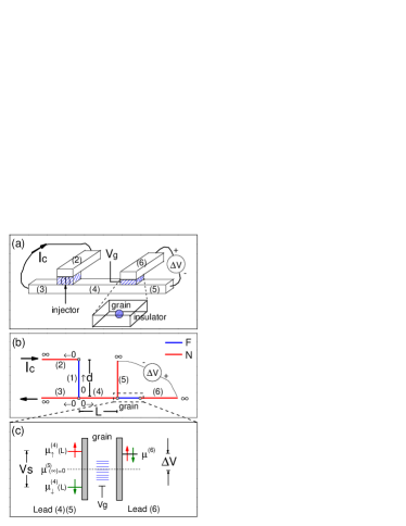
Figure 1: (a) The schematic of our non-local spin valve (NLSV) device. It can be viewed as a combination of the setups employed in Ref. Yang et al., 2008 and Ref. Deshmukh et al., 2001. (b) The device is separated into 7 regions. (1) is a fixed ferromagnetic injector of thickness $d$. The ferromagnetic grain on the right is to be manipulated and detected. The distance between (1) and the grain is $L$. “ $0\rightarrow$ ” in each region defines the local origin and positive direction of coordinate. (c) The grain and its nearby regions is modeled as a Stoner particle coupled to two non-magnetic lead via tunneling through two barriers. Driven by the spin-polarized current $I_{c}$, spins injected from (1) accumulate and induce a splitting ($V_{s}$) of the spin-up and down chemical potentials [$\mu_{\uparrow/\downarrow}^{(4)}(L)$] at the (4)/(5)/grain interface. $V_{g}$ is the gate voltage applied to the insulator [see Fig. 1(a)] surrounding the grain, much like the technique in Ref. Deshmukh et al., 2001. In this way, it can be used to tune the energy levels inside the grain with respect to chemical potentials of (4), (5), and (6) capacitively, while without inducing direct current between the gate and the grain. $\Delta V$ measures the voltage between (5) and (6), and is defined as the NLSV voltage. $\mu^{(5)}(\infty)$ is the chemical potential at the voltmeter side of regions (5), and is set as the energy zero point throughout the paper.

II.1 General survey of our setup

The device we study is shown in Fig. 1(a), which can be divided into 7 regions, “(1)-(6)” and “grain”, as shown in Fig. 1(b). The different regions of the device are separated into three parts, and modeled by different formalisms, depending on their sizes and positions:

(i) the first part consists of regions (1)-(5). Their sizes are comparable to their spin diffusion lengthes, thus the spin transport in these regions are governed by the spin diffusion equations.van Son et al. (1987); Valet and Fert (1993); Hershfield and Zhao (1997); Jedema et al. (2003); Takahashi and Maekawa (2003) The magnetization of injector (1) is assumed to be fixed.

(ii) the second part is the smaller ( approximately several nm) grain, which is described as a Stoner particle,Canali and MacDonald (2000); Kleff et al. (2001) coupled via sequential tunneling to two nonmagnetic leads. For convenience, we call them lead (4,5) and lead (6), respectively. Lead (4,5) and lead (6) are defined as where regions (4) and (5) and region (6) connect the grain, respectively. We assume that there is no direct tunneling between lead (4,5) and lead (6), i.e., the only possible connection between them is via the grain.

(iii) The third part is floating region (6). Because of the voltmeter, it is an open circuit between regions (4) and (5) and region (6), i.e., at steady state, there is no current flowing from regions (4) and (5) across the grain to (6), due to a voltage difference between (6) and (5). Throughout the paper, we define the chemical potential $\mu^{(5)}(\infty)$ at the voltmeter side of region (5) as the energy zero point. The chemical potential of region (6) is denoted as $\mu^{(6)}$. The difference between $\mu^{(6)}$ and $\mu^{(5)}(\infty)$ is denoted as $\Delta V\equiv\mu^{(6)}-\mu^{(5)}(\infty)$, where $\Delta V$ is the NLSV voltage. $\Delta V$ will be determined through self-consistent calculation.

In a word, our model can be viewed as a combination of the setup used in two kinds of experiments, i.e., the NLSVYang et al. (2008) and the transport through ferromagnetic nanograins. Guéron et al. (1999); Deshmukh et al. (2001) Besides:

(i) Different from usual ferromagnetic nanograins setups,Guéron et al. (1999); Deshmukh et al. (2001) the chemical potentials for spin-up and -down electrons $\mu_{\uparrow/\downarrow}^{(4)}(L)$ are split at the (4)/(5)/grain interface, as shown in Fig. 1(c). The splitting is called the spin bias, and denoted as $V_{s}$.Wang et al. (2004); Sun et al. (2008); Lu and Shen (2008); Lu et al. (2009); Xing et al. (2008); Stefanucci et al. (2008) This spin bias is induced by the spins injected from region (1) to region (4). Later in Secs. III and IV.1, we will see that $V_{s}$ is crucial to the detection of NLSV signal and the magnetization reversal, thus we will first evaluate its magnitude in the following subsection.

(ii) Different for usual NLSVs,Kimura et al. (2006); Yang et al. (2008) The ultrasmall size of the grain allows the NLSV signal, the magnetization reversal dynamics, and the interaction between the currents and the grain to be described within one set of rate equations Eq. (12).

For a better understanding of our setup, the calculation steps of the magnetization and the NLSV signal as functions of $I_{c}$ is presented in Fig. 2. This section is organized as follows. In Sec. II.2, $V_{s}$ will be estimated with realistic experimental parameters. In Sec. II.3, the description of the grain will be introduced. In Sec. II.4, the transport between the grain and its leads will be described by the rate equations. The details of theoretical descriptions can be found in Appendixes A-C, and will be specified in the following subsections.

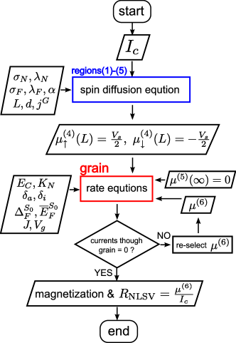
Figure 2: The calculation steps of the magnetization of the grain and the non-local spin valve signal $R_{\mathrm{NLSV}}$ as functions of $I_{c}$, the driving current. Rectangles represent calculation processes. Parallelograms represent inputs or outputs of the calculations. The region (1), (2), (3), (4) and (5) in Fig. 1 are described by the spin diffusion equation given by Eq. (II.2). The grain and its nearby regions are described by the rate equations given by Eq. (12). The diamond represents the self-consistent calculation of $\mu^{(6)}$, the chemical potential of region (6).

II.2 Spin diffusion transport in regions (1)-(5) and estimate of spin bias $V_{s}$

In this section, we will estimate the magnitude of $V_{s}$, which is defined as the splitting of spin-up and -down chemical potentials at the (4)/(5)/grain interface,

$$V_{s}\equiv\mu_{\uparrow}^{(4)}(L)-\mu_{\downarrow}^{(4)}(L)\equiv\mu_{\uparrow}^{(5)}(0)-\mu_{\downarrow}^{(5)}(0).$$ (1)

Following the previous literatures, the spin and charge transports in regions (1)-(5) are described by the standard diffusion equation,van Son et al. (1987); Valet and Fert (1993); Hershfield and Zhao (1997); Jedema et al. (2003); Takahashi and Maekawa (2003)

$$\nabla^{2}(\sigma_{\uparrow}\mu_{\uparrow}+\sigma_{\downarrow}\mu_{\downarrow}) = 0,$$

$$\nabla^{2}(\mu_{\uparrow}-\mu_{\downarrow}) = \frac{1}{\lambda^{2}}(\mu_{\uparrow}-\mu_{\downarrow}),$$ (2)

where $\lambda$ is a phenomenological spin-diffusion length that can be measured experimentally.Bass and Jr (2007) Usually, the spin-diffusion length in normal metal is much longer than that in ferromagnetic metal, i.e., $\lambda_{N}\gg\lambda_{F}$. In this work, we use $\lambda_{N}=1000$ nm, and $\lambda_{F}=5$ nm.Yang et al. (2008) $\sigma_{\sigma}$ is the conductivity for $\sigma$ electrons. For ferromagnetic metal, $\sigma_{\uparrow}=\sigma_{F}(1+\alpha)/2$ and $\sigma_{\downarrow}=\sigma_{F}(1-\alpha)/2$, where $\sigma_{F}$ is the total conductivity of the ferromagnetic metal, $\alpha$ is the bulk polarization defined as $\alpha\equiv(\sigma_{\uparrow}-\sigma_{\downarrow})/(\sigma_{\uparrow}+\sigma_{\downarrow})$. For normal metal, $\sigma_{\uparrow}=\sigma_{\downarrow}=\sigma_{N}/2$. In this work, we use $\sigma_{N}=8.8\times 10^{7}\Omega^{-1}\mathrm{m}^{-1}$, $\sigma_{F}=9.8\times 10^{6}\Omega^{-1}\mathrm{m}^{-1}$, and $\alpha=0.2$.Kimura et al. (2006)

We calculate the chemical potentials in regions (1)-(5) of Fig. 1(b), where regions (2), (3), and (5) can be regarded as semi-infinite. By assuming that the same cross-section area $A_{\Box}$ perpendicular to the current in each region, the solutions to Eq. (II.2) can be simplified to be one dimensional. Following Jedema et al.,Jedema et al. (2003) the general solutions to the 5 regions as functions of position $x$ are given by

$$\mu_{\uparrow/\downarrow}^{(1)} = A+\frac{ej_{c}}{\sigma_{F}}x\pm\frac{B}{\sigma_{F}(1\pm\alpha)}e^{-\frac{x}{\lambda_{F}}}\pm\frac{C}{\sigma_{F}(1\pm\alpha)}e^{\frac{x}{\lambda_{F}}},$$

$$\mu_{\uparrow/\downarrow}^{(2)} = D+\frac{ej_{c}}{\sigma_{N}}x\pm\frac{E}{\sigma_{N}}e^{-x/\lambda_{N}},$$

$$\mu_{\uparrow/\downarrow}^{(3)} = -\frac{ej_{c}}{\sigma_{N}}x\pm\frac{F}{\sigma_{N}}e^{-x/\lambda_{N}},$$

$$\mu_{\uparrow/\downarrow}^{(4)} = \pm\frac{G}{\sigma_{N}}e^{-x/\lambda_{\mathrm{N}}}\pm\frac{H}{\sigma_{N}}e^{x/\lambda_{N}},$$

$$\mu_{\uparrow/\downarrow}^{(5)} = \pm\frac{K}{\sigma_{N}}e^{-x/\lambda_{\mathrm{N}}},$$ (3)

where the origin and positive direction in each region are locally defined for a concise form of the general solutions, and indicated by “ $0\rightarrow$ ” in Fig. 1(b). $j_{c}=I_{c}/A_{\Box}$, where $I_{c}$ is the spin-polarized total current flowing through regions (2), (1), and (3). $e$ is the electron charge. The 9 coefficients $A$, $B$, $C$, $D$, $E$, $F$, $G$, $H$, and $K$ will be determined by boundary conditions.

The boundary conditions are given as follows:

(i) The current polarization usually loses when flowing through an interface from the ferromagnetic to the normal side, due to, e.g., the spin-dependent scattering. We take this loss into account by phenomenologically introducing an efficiency parameter $\gamma\in[0,1]$,

$$\gamma\frac{j_{F\uparrow}-j_{F\downarrow}}{j_{F\uparrow}+j_{F\downarrow}}=\frac{j_{N\uparrow}-j_{N\downarrow}}{j_{N\uparrow}+j_{N\downarrow}},$$ (4)

where $j_{\sigma}=-(\sigma_{\sigma}/e)\partial_{x}\mu_{\sigma}$, is the current density for the spin-$\sigma$ electrons. By combining Eq. (4) and the conservation of the total current

$$j_{F\uparrow}+j_{F\downarrow}=j_{N\uparrow}+j_{N\downarrow},$$ (5)

the boundary conditions at the ferromagnetic/normal interface are then given by,

$$j_{F\uparrow}=\frac{\gamma+1}{2\gamma}j_{N\uparrow}+\frac{\gamma-1}{2\gamma}j_{N\downarrow},$$

$$j_{F\downarrow}=\frac{\gamma+1}{2\gamma}j_{N\downarrow}+\frac{\gamma-1}{2\gamma}j_{N\uparrow}.$$ (6)

(ii) The chemical potentials of each spin components are continuous at each interface. For simplicity, we do not explicitly include the spin-dependent chemical potential drops caused by the interface resistance. Its destructive effects, in particular on the reduction in the spin bias, will be approximately accounted by considering a relatively small injection efficiency $\gamma$.

(iii) At the (4)/(5)/grain interface, the spin-up and -down currents flowing into the grain are $I^{G}$ and $-I^{G}$, respectively, i.e., (how this boundary condition is derived can be found in Appendix A)

$$-A_{\Box}\frac{\sigma_{N}}{2}\partial_{x}\mu_{\uparrow/\downarrow}^{(4)}(L)=\pm eI^{G}-A_{\Box}\frac{\sigma_{N}}{2}\partial_{x}\mu_{\uparrow/\downarrow}^{(5)}(0),$$ (7)

where we assume a pure spin current flowing from (4) and (5) into the grain, which however may not be true as we will see in Sec. IV.2. However, this deviation is neglected because $I^{G}$ is too small to affect $V_{s}$, as we will see in Sec. IV.3. Actually, because $I^{G}$ is ignorably small, we simply neglect it in our numerical calculations, though we include it in equations explicitly.

With these boundary conditions, the coefficients from $A$ through $K$ in Eq. (II.2) are readily found. Figs. 3(a) and 3(b) show the spin-resolved chemical potentials $\mu_{\uparrow}$ and $\mu_{\downarrow}$ in regions (1)-(5). For a clear demonstration of the splitting between spin-up and -down chemical potentials, we choose $\alpha=0.9$ only in these two figures. For the realistic evaluations in the rest part of this work, we choose $\alpha=0.2$, as estimated by the experiments.Kimura et al. (2006); Yang et al. (2008) All the conductivities, spin-diffusion lengthes, and the bulk polarization used for the evaluation are extracted from the experiment data,Kimura et al. (2006); Yang et al. (2008) and given in Fig. 3. Driven by $I_{c}$, the spins injected from injector (1) induce a splitting between $\mu_{\uparrow}$ and $\mu_{\downarrow}$ at interfaces (1)/(2) and (1)/(3)/(4). Because injector (1) is sandwiched between two normal metals, $\mu_{\uparrow}$ and $\mu_{\downarrow}$ in (1) cross with each other at the center and split oppositely on the opposite sides. In each region of (1), (2), and (3), because of the charge current $I_{c}$, $\mu_{\uparrow}$ and $\mu_{\downarrow}$ not only split but also demonstrate steep slopes with the same trend. Because of no net charge current, $\mu_{\uparrow}$ and $\mu_{\downarrow}$ in region (4) just diffuse to the right side in opposite gradients (not obvious here because $L\ll\lambda_{N}$).

By using Eq. (1), the analytic expression for $V_{s}$ is found out as

$$V_{s} \equiv \mu_{\uparrow}^{(4)}(L)-\mu_{\downarrow}^{(4)}(L)\equiv\mu_{\uparrow}^{(5)}(0)-\mu_{\downarrow}^{(5)}(0),$$ (8)

$$= 2ej_{c}\frac{\lambda_{F}}{\sigma_{F}}\frac{\alpha}{(1-\alpha^{2})}\frac{(M_{1}-2)}{M_{2}}e^{-\frac{L}{\lambda_{N}}}$$

$$- 2e\frac{I^{G}}{A_{\Box}}[\frac{\lambda_{F}}{\sigma_{F}}\frac{2e^{-\frac{2L}{\lambda_{N}}}M_{1}}{\gamma(1-\alpha^{2})M_{2}}+\frac{\lambda_{N}}{\sigma_{N}}(1-e^{-\frac{2L}{\lambda_{N}}})],$$

where

$$M_{1} = 2\cosh(\frac{d}{\lambda_{F}})+2M_{0}\sinh(\frac{d}{\lambda_{F}}),$$

$$M_{2} = 6M_{0}\cosh(\frac{d}{\lambda_{F}})+2(2M_{0}^{2}+1)\sinh(\frac{d}{\lambda_{F}}),$$

$$M_{0} = \frac{\sigma_{N}\lambda_{F}}{\sigma_{F}\lambda_{N}\gamma(1-\alpha^{2})}.$$ (9)

Figures. 3(c)-(e) show the spin bias $V_{s}$ as a function of $I_{c}$ and $\gamma$. Later we will see in Secs. IV.2 and IV.3 that $I^{G}$ is ignorably small, thus hardly changing $V_{s}$. Thus, we let $I^{G}=0$. As we see, $V_{s}$ can be as large as $\sim 0.1$ meV for the present device and parameters. $V_{s}$ increases linearly with $I_{c}$, while logarithmically with $\gamma$. $V_{s}$ changes sign with the current $I_{c}$.

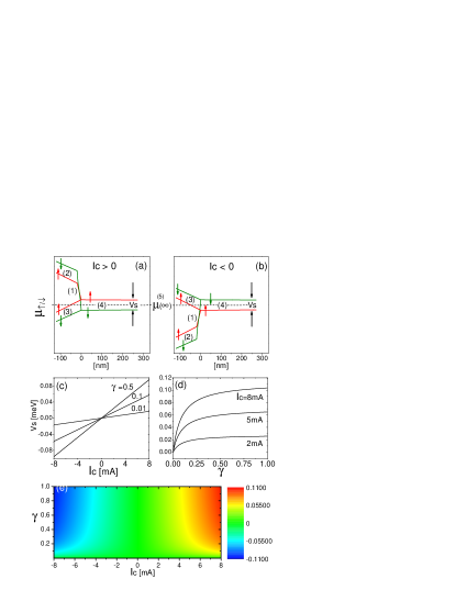
Figure 3: (a)(b): The chemical potentials $\mu_{\uparrow}$ (marked by $\uparrow$) and $\mu_{\downarrow}$ (marked by $\downarrow$) in regions (1)-(4). They change with the direction of $I_{c}$, the spin-polarized current flowing through regions (1), (2), and (3). $V_{s}$ is defined as $\mu_{\uparrow}-\mu_{\downarrow}$ at the (4)/(5)/grain interface. The horizontal dashed line indicates $\mu^{(5)}(\infty)$, the energy zero point throughout the paper. (c) $V_{s}$ vs $I_{c}$ for different values of spin injection efficiency $\gamma$. (d) $V_{s}$ vs $\gamma$ for different $I_{c}$. (e) $V_{s}$ (in unit of meV) as a function of $I_{c}$ and $\gamma$. The parameters for (c)(d)(e): $d=20$ nm, $L=270$ nm, $A_{\Box}=170\times 65\ \mathrm{nm}^{2}$, $\lambda_{F}=5$ nm, $\lambda_{N}=1000$ nm, $\sigma_{F}=9.8\times 10^{6}\ \Omega^{-1}\mathrm{m}^{-1}$, $\sigma_{N}=8.8\times 10^{7}\ \Omega^{-1}\mathrm{m}^{-1}$, $\alpha=0.2$, $I^{G}=0$.

In the following, for a conservative and realistic simulation, we will always choose a relatively low injection efficiency $\gamma=0.1$ and assume $I^{G}=0$. Since the above boundary conditions only consider the conservation of current density, our results are valid when assuming the identical cross-section area in each part of the setup. One should consider different cross section area in different regions and current conservation for a more general case.Takahashi and Maekawa (2003)

II.3 Many-body states of the ferromagnetic nanograin

In this work, we will describe the ferromagnetic nanograin by using the minimal possible modelCanali and MacDonald (2000); Kleff et al. (2001) proposed to describe the experiment transport spectra through cobalt nanograin.Guéron et al. (1999); Deshmukh et al. (2001) This model was also adopted to discuss spin-polarized current-induced relaxation and spin torque in the ferromagnetic nanograin.Waintal and Brouwer (2003); Waintal and Parcollet (2005); Parcollet and Waintal (2006)

A full and detailed description of this model can be found in Appendix B. Simply speaking, at low temperatures, the grain can be described by the many-body states $|N,S,S_{z}\rangle$, where $N$ is the total electron number inside the grain, $S$ and $S_{z}$ are the magnitude and the $z$-component of the total angular momentum $\mathbf{S}$ of the grain, respectively.

In the following, we will focus on two branches of states. The first branch is

$$|N_{0},S_{0},S_{z}\rangle,$$ (10)

i.e., there are $N=N_{0}$ electrons inside the grain, and the magnitude of the total angular momentum of the grain is $S=S_{0}$. Besides, since $S_{z}\in[-S_{0},S_{0}]$, there are $2S_{0}+1$ states in this branch. The second branch is obtained by adding an extra electron to the minority band of the grain with respect to the first branch, so that the total electron number increases by 1 and the magnitude of the total angular momentum decreases by $1/2$. This branch is denoted as

$$|N_{0}+1,S_{0}-1/2,S_{z}\rangle,$$ (11)

where $S_{z}\in[-S_{0}+1/2,S_{0}-1/2]$, i.e., there are $2S_{0}$ states in this branch.

We refer regions (4)-(6) as the two “leads” connected to the grain, one is from regions (4) and (5), the other is from region (6). By tuning the gate voltage $V_{g}$ and applying the spin bias $V_{s}$ (induced by $I_{c}$), the energies of the two branches presented in Eqs. (10) and (11) can be set to be nearly degenerate with respect to the chemical potentials $\mu^{(4)}_{\uparrow,\downarrow}(L)$, $\mu^{(5)}_{\uparrow,\downarrow}(0)$, and $\mu^{(6)}$. In this situation, the electrons in lead (4,5) and lead (6) can be exchanged with the grain. Then we can use the polarization of the exchanged electrons to detect and manipulate the magnetization of the ferromagnetic grain.

Figure 4: The easy-axis of the grain is set as $z$ direction. The grain electrons ($d_{i\uparrow/\downarrow}$) are quantized along $z$ direction. The majority and minority electrons orient parallel and anti-parallel with $\mathbf{S}$, respectively. $\mathbf{S}$ is the total angular momentum of the grain formed by all the electrons inside the grain. $\theta$ is the angle between the easy axis of grain and the spin-quantization direction of lead (4,5).

II.4 Rate equations in the presence of spin bias

The evolution of the many-body states of the grain by exchanging electrons with the weakly coupled lead (4,5) and lead (6) is described by the Pauli rate equations.Beenakker (1991); Blum (1996); von Delft and Ralph (2001) We only consider the sequential tunneling regime. Born approximation and Markoff approximation are applied, and $H_{\mathrm{T}}$ is treated by perturbation up to the second order.Blum (1996) The rate equation can be expressed in a compact form,

$$\partial_{t}P_{l}=\sum_{l^{\prime}}R_{ll^{\prime}}P_{l^{\prime}},$$ (12)

where $0\leq P_{l}\leq 1$ are the probability to find the state $l\equiv|N,S,S_{z}\rangle$. The diagonal and off-diagonal terms of the coefficient matrix of the rate equations are, respectively,

$$R_{l^{\prime}\neq l}=\sum_{\alpha\sigma i}R_{l^{\prime}\neq l}^{\alpha\sigma i},\ \ R_{ll}=-\sum_{l^{\prime}\neq l}R_{l^{\prime}l},$$ (13)

where

$$R_{l^{\prime}\neq l}^{\alpha\uparrow i} = \Gamma_{\alpha}\cos^{2}\frac{\theta_{\alpha}}{2}[|\langle l^{\prime}|d_{i\uparrow}|l\rangle|^{2}f(E_{l}-E_{l^{\prime}}-\mu_{+}^{\alpha})$$ (14)

$$\ \ \ \ \ \ \ \ \ \ \ +|\langle l|d_{i\uparrow}|l^{\prime}\rangle|^{2}f(E_{l}-E_{l^{\prime}}+\mu_{+}^{\alpha})]$$

$$+\Gamma_{\alpha}\sin^{2}\frac{\theta_{\alpha}}{2}[|\langle l^{\prime}|d_{i\uparrow}|l\rangle|^{2}f(E_{l}-E_{l^{\prime}}-\mu_{-}^{\alpha})$$

$$\ \ \ \ \ \ \ \ \ \ \ +|\langle l|d_{i\uparrow}|l^{\prime}\rangle|^{2}f(E_{l}-E_{l^{\prime}}+\mu_{-}^{\alpha})],$$

and one just replaces $\uparrow$ with $\downarrow$ and exchanges $+$ and $-$ to obtain $R_{l^{\prime}l}^{\alpha\downarrow i}$. Note that the Fermi distribution $f(x)=1/[\exp(x/k_{B}T)+1]$ is spin-resolved. The parameter $\Gamma_{\alpha}=2\pi\sum_{k}|V_{k\alpha i}|^{2}\delta(\omega-\epsilon_{k\alpha})$ represents the spin-irrelevant coupling between lead $\alpha\in\{(4,5),(6)\}$ and the grain. For simplicity, we assume that $\Gamma_{(4,5)}=\Gamma_{(6)}=\Gamma$, and $\Gamma$ are assumed to be independent of the specific single-particle level $i$. The overlapping $\langle l|d_{i\sigma}|l^{\prime}\rangle$ can be found by calculating the Clebsch-Gordan coefficients.

$\theta_{\alpha}$ in Eq. (14) is the angle between the easy axis of grain and the spin-quantization direction of lead $\alpha$. For simplicity, we set the easy-axis of the grain as $z$-axis and assume that $\theta_{(6)}=0$ and $\theta_{(4,5)}=\theta\in[0,\pi/2]$, as shown in Fig. 4. In the following, we denote $\mu_{+/-}^{(4)}=\mu_{\uparrow/\downarrow}^{(4)}$ when $\theta=0$.

In terms of $P_{l}$, the magnetization of the grain is given by

$$M=\sum_{l}S_{z}^{l}P_{l},$$ (15)

and the spin-$\sigma$ current flowing from region $\alpha$ into the grain are defined as

$$I_{\alpha}^{\sigma}=-e\sum_{ll^{\prime}}(N_{l}-N_{l^{\prime}})R_{l^{\prime}l}^{\alpha\sigma}P_{l^{\prime}},$$ (16)

where $N_{l}$ and $S_{z}^{l}$ correspond to the $N$ and $S_{z}$ of the state $l\equiv|N,S,S_{z}\rangle$.

The validity of the rate equations is discussed in Appendix C.

III NLSV signal in the tunneling regime

In this section, we will present the microscopic picture of the NLSV signal in the sequential tunneling regime. When a small current $I_{c}$ is driven in the loop formed by regions (1)-(3) of Fig. 1(a), the relative alignment of magnetization between the two ferromagnets can be read out by measuring the voltage difference between regions (6) and (5).

III.1 $\theta=0$ case

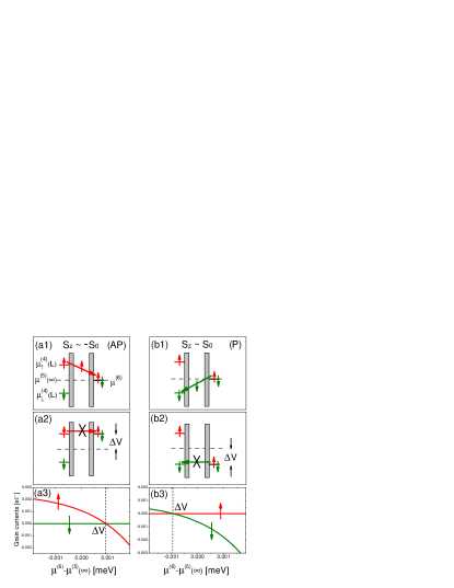
Figure 5: Using NLSV signal in the sequential tunneling regime to read out the magnetization of the grain. (a1)-(a3) and (b1)-(b3) show the cases when the magnetization of the grain is antiparallel (AP) and parallel (P) with injector (1), respectively. $\mu^{(5)}(\infty)$ and $\mu^{(6)}$ are the chemical potentials on the voltmeter side of regions (5) and (6), respectively. (a1) When $S_{z}\sim-S_{0}$, the grain favors spin-up current flowing from lead (4,5) to lead (6). Because it is an open circuit between lead (4,5) and lead (6), the electrons flowing into lead (6) can not go anywhere but build up and raise the chemical potential $\mu^{(6)}$. (a2) Once the chemical potential $\mu^{(6)}$ is raised to be aligned with $\mu^{(4)}_{\uparrow}(L)$, the current flowing and electron building-up stop. Then one can measure a voltage difference between $\mu^{(5)}(\infty)$ and $\mu^{(6)}$, which corresponds to the NLSV voltage. (a3) The spin-up and -down currents as functions of $\mu^{(6)}-\mu^{(5)}(\infty)$. The NLSV voltage $\Delta V=\mu^{(6)}-\mu^{(5)}(\infty)$ corresponds to the vertical dashed line at which both currents are zero. (b1)-(b3) can be understood similarly. The parameters: $\theta=0$, $I_{c}=250\ \mu$A, $\gamma=0.1$, $I^{G}=0$, $S_{0}=100$, $T=20$ mK, $\Delta V_{g}=-K_{N}$, and other parameters are the same as those in Fig. 3.

We will discuss first the case when $\theta=0$. For $\theta=0$, we denote $\mu_{+/-}^{(4)}=\mu_{\uparrow/\downarrow}^{(4)}$. The results can be easily generalized for $\theta\neq 0$ in Sec. III.2. The left and right columns of Fig. 5 show the cases when the magnetization of the grain is anti-parallel (AP) and parallel (P) with injector (1), respectively. First, we consider the AP case, i.e., $S_{z}$ of the grain $\sim-S_{0}$. By putting the experimental measurement currentYang et al. (2008) $I_{c}=$250 $\mu$A into Eq. (8) and assuming $\gamma=0.1$ and $I^{G}=0$, we estimate that a positive spin bias $V_{s}\sim$ 1.84 $\mu$eV will be induced at the interface where regions (4), (5) and the grain connect, so that $\mu^{(4)}_{\uparrow/\downarrow}(L)=\mu^{(5)}_{\uparrow/\downarrow}(0)=\pm V_{s}/2$. It is natural to assume that the distance between the voltmeter and the (4)/(5)/grain interface $\gg\lambda_{N}=1\ \mu$m, so the split chemical potentials for spin-up and -down electrons will decay to only one chemical potential $\mu^{(5)}(\infty)$ on the voltmeter side of region (5). Because region (5) is nonmagnetic, the decays of spin-up and -down chemical potentials are symmetric, so it can be anticipated that $\mu^{(5)}(\infty)=[\mu^{(4)}_{\uparrow}(L)+\mu^{(4)}_{\downarrow}(L)]/2=[\mu^{(5)}_{\uparrow}(0)+\mu^{(5)}_{\downarrow}(0)]/2$. This situation is depicted by $\mu^{(4)}_{\uparrow/\downarrow}(L)$ and $\mu^{(5)}(\infty)$ in Fig. 5 (a1).

In the response of this small spin bias, a small current will be generated, flowing through the grain. Specifically, spin-up current will be favored for the AP case. This can be understood with the help of the Clebsch-Gordan coefficient,

$$\langle N_{0},S_{0},S_{z}|d_{i\uparrow}|N_{0}+1,S_{0}-\frac{1}{2},S_{z}+\frac{1}{2}\rangle$$ (17)

$$= \langle j_{1}=S_{0},m_{1}=S_{z};j_{2}=\frac{1}{2},m_{2}=\frac{1}{2}$$

$$|J=S_{0}-\frac{1}{2},M=S_{z}+\frac{1}{2}\rangle$$

$$= -\sqrt{\frac{S_{0}-S_{z}}{2S_{0}+1}}$$

$$\langle N_{0},S_{0},S_{z}|d_{i\downarrow}|N_{0}+1,S_{0}-\frac{1}{2},S_{z}-\frac{1}{2}\rangle$$

$$= \langle j_{1}=S_{0},m_{1}=S_{z};j_{2}=\frac{1}{2},m_{2}=-\frac{1}{2}$$

$$|J=S_{0}-\frac{1}{2},M=S_{z}-\frac{1}{2}\rangle$$

$$= \sqrt{\frac{S_{0}+S_{z}}{2S_{0}+1}},$$

apparently, for $S_{z}\sim-S_{0}$, the probability for spin-up electrons to tunnel through the grain

$$\frac{S_{0}-(-S_{0})}{2S_{0}+1}\sim 1,$$ (18)

is much larger than the probability for spin-down electrons

$$\frac{S_{0}+(-S_{0})}{2S_{0}+1}\sim 0.$$ (19)

In other words, the spin-down current is magnetic blockaded.Waintal and Parcollet (2005) Note that the spin selection rules remain qualitatively unchanged even for small fluctuation of $S_{z}$ around $-S_{0}$, as long as $S_{0}\gg 1$.

As a result, the favored spin-up electrons will flow from region (4) through the grain into region (6), if $\mu^{(4)}_{\uparrow}(L)>\mu^{(6)}$. Remember that there is a voltmeter between regions (5) and (6), so the electrons tunneling into region (6) can not go anywhere but accumulate and raise the chemical potential of region (6) until $\mu^{(6)}\sim\mu^{(4)}_{\uparrow}(L)$. After this accumulation is accomplished, no more current will flow and there is finally a stable voltage difference $\Delta V$ between $\mu^{(6)}$ and $\mu^{(5)}(\infty)$, as shown in Fig. 5 (a2).

Fig. 5 (a3) shows how to numerically determine the NLSV voltage $\Delta V$. One just scan $\mu^{(6)}$ and calculate the tunneling current through the grain. $\Delta V$ is then found out as at which $\mu^{(6)}-\mu^{(5)}(\infty)$ both the spin-up and -down currents vanish, as indicated by the vertical dashed line. It turns out that in the sequential tunneling regime and when $\theta=0$, the magnitude of the NLSV voltage is

$$|\Delta V^{\theta=0}| = |V_{s}|/2.$$ (20)

By using Eq. (8) and the parameters given in Fig. 5, for $I_{c}=250\ \mu$A, the NLSV voltage $\Delta V^{\theta=0}$ is found out to be about 0.92 $\mu$V. The NLSV signal is thereby equal to

$$R_{\mathrm{NLSV}}^{\theta=0}\equiv\frac{\Delta V^{\theta=0}}{I_{c}}=\frac{0.92\ \mu\mathrm{V}}{250\mu\mathrm{A}}\simeq 3.7\mathrm{m}\Omega.$$ (21)

Similarly, as shown in Figs. 5 (b1)-(b3), the parallel (P) case favors that spin-down current flowing from region (6) through the grain to regions (4) and (5), also due to the same spin selection rules Eq. (17). This current will drain the electrons in region (6) and lower $\mu^{(6)}$ until $\mu^{(6)}\sim\mu^{(4)}_{\downarrow}(L)$. Therefore, for the P case, $\Delta V^{\theta=0}=-0.92\mu$eV and $R^{\theta=0}_{\mathrm{NLSV}}=-3.7$m$\Omega$, right opposite to the AP case.

III.2 $\theta\neq 0$ case

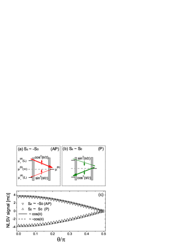
Figure 6: NLSV signal when $\theta\neq 0$. (a) when $\theta\neq 0$ and the magnetization of the grain is $S_{z}=-S_{0}$ (AP), the spin-up current can flow simultaneously from lead (4,5) to lead (6) with relative probability $\cos^{2}\frac{\theta}{2}$, and from lead (6) to lead (4,5) with probability $\sin^{2}\frac{\theta}{2}$. (b) when $\theta\neq 0$ and the magnetization of the grain is $S_{z}=S_{0}$ (P), spin-down current can flow simultaneously from lead (4,5) to lead (6) with relative probability $\sin^{2}\frac{\theta}{2}$, and from lead (6) to lead (4,5) with probability $\cos^{2}\frac{\theta}{2}$. (c) The NLSV signal as a function of $\theta$ for the P ($\triangle$) and AP ($\nabla$) cases. $\pm\cos\theta$ are also plotted for comparison. Other parameters are the same as Fig. 5.

When $\theta\neq 0$, the chemical potentials of lead (4,5) now are denoted as $\mu_{+}^{(4)}(L)$ and $\mu_{-}^{(4)}(L)$, respectively. We still take $S_{z}\sim-S_{0}$ for example. As shown in Fig. 6(a), when $\theta\neq 0$, the favored spin-$\uparrow$ current can flow not only from $\mu_{+}^{(4)}(L)$ to $\mu^{(6)}$, but also from $\mu^{(6)}$ to $\mu_{-}^{(4)}(L)$, according to the rate equations Eq. (14). These two currents are denoted as $I^{\uparrow}_{\mu_{+}^{(4)}(L)\rightarrow\mu^{(6)}}$ and $I^{\uparrow}_{\mu^{(6)}\rightarrow\mu_{-}^{(4)}(L)}$, respectively.

According to the rate coefficients Eq. (14), the spin-up electrons are related to $\mu^{(4)}_{+}(L)$ by $\cos^{2}\frac{\theta}{2}$, and to $\mu^{(4)}_{-}(L)$ by $\sin^{2}\frac{\theta}{2}$. Besides, lead (6) is not spin-dependent, so the polarization and magnitude of the current between the grain and (6) just follow those between (4) and the grain. Therefore,

$$I^{\uparrow}_{\mu_{+}^{(4)}(L)\rightarrow\mu^{(6)}} \propto \cos^{2}\frac{\theta}{2},$$

$$I^{\uparrow}_{\mu^{(6)}\rightarrow\mu_{-}^{(4)}(L)} \propto \sin^{2}\frac{\theta}{2},$$ (22)

respectively. As a result, $\mu^{(6)}$ will saturate to a balanced position at which the above two opposite currents cancel with each other. Because $\cos^{2}\frac{\theta}{2}-\sin^{2}\frac{\theta}{2}=\cos\theta$, this balanced position of $\mu^{(6)}$ turns out to be proportional to $\cos\theta$.Kimura et al. (2007)

The triangles in Fig. 6(c) show the self-consistent results of the NLSV signal as a function of $\theta$. For comparison, the functions $\pm\cos\theta$ are also plotted by solid and dashed lines, respectively. One easily concludes that the NLSV signal in the presence of $\theta$ is given by

$$R_{\mathrm{NLSV}}=\pm\frac{V_{s}}{2I_{c}}\cos\theta,$$ (23)

where $\pm$ depends on the magnetization of the grain.

III.3 Discussion

There are several points should be clarified:

(i) $R_{\mathrm{NLSV}}$ we obtained for the present device and parameters happen to be of the same order as the experimental observations, where the NLSV signals are of the order of $1\sim 10$ m$\Omega$.Yang et al. (2008)

(ii) Above, we only consider the case that $S$ decreases by $1/2$ when the extra electron is added, where $S$ is the magnitude of the total angular momentum of the grain. Also, according to Fig. 11, there is small probability that $S$ increases by $1/2$ when adding the extra electron, i.e., the extra electron is preferred to be added to the majority band, then the spin selection rules will become totally reversed as

$$\langle N_{0},S_{0},S_{z}|d_{i\uparrow}|N_{0}+1,S_{0}+\frac{1}{2},S_{z}+{\frac{1}{2}}\rangle = \sqrt{\frac{S_{0}+S_{z}+1}{2S_{0}+1}},$$

$$\langle N_{0},S_{0},S_{z}|d_{i\downarrow}|N_{0}+1,S_{0}+\frac{1}{2},S_{z}-{\frac{1}{2}}\rangle = \sqrt{\frac{S_{0}-S_{z}+1}{2S_{0}+1}},$$

so that tunneling of spin-up (spin-down) electrons will be favored when $S_{z}\sim S_{0}$ ($S_{z}\sim-S_{0}$). Therefore, the results will be totally reversed. This is a direct consequence of the strong Coulomb repulsion and the unequal spacings $\delta_{a}$ and $\delta_{i}$ of majority and minority one-particle levels for an ultrasmall grain, and a major difference from the relatively large films.Kimura et al. (2006); Yang et al. (2008)

(iii) Note that in regions (4) and (5), the stead-state splitting of spin-up and -down chemical potentials is maintained by the spins continuously injected by $I_{c}$. This is different from in region (6), where there should be no current flowing in or out at steady state, because of the voltmeter. Therefore, in region (6), the spin-up and -down electrons will eventually relax to one chemical potential for sufficient long time. That is why we consider, for the steady-state solution, only one spin-irrelevant chemical potential $\mu^{(6)}$ in region (6).

(iv) In the simulation, although the parameters listed in Table 1 for a $S_{0}=1000$ grain are exploited, we only use $S_{0}=100$ for simulation because of the limited computing power. We have checked the results from $S_{0}=10$ through $S_{0}=100$, and the results turn out to be quantitatively unchanged as long as $S\gg 1$.

IV Magnetization Switching

In this section, we will present the magnetization switching of the grain under a current $I_{c}$ exceeding a critical value. This critical $I_{c}$ is determined by the gate voltage $V_{g}$ and the spin bias $V_{s}$, at which the strong Coulomb and magnetic blockades of the grain are lifted. Then currents can flow through the grain, and transfer the angular momentum carried by the flowing electrons to the grain. This will be discussed in Sec. IV.1.

Besides, still because of these blockades, one can not pre-assume there is always a pure spin current flowing through the grain, so whether the reversal is accompanied by the pure spin current is waited to be checked. This will be discussed in Sec. IV.2.

IV.1 Critical $I_{c}$ and $V_{s}$

Figure 7: (a) The spin bias $V_{s}$, (b) the normalized magnetization, (c) the NLSV voltage, and (d) the NLSV signal as functions of the driving current $I_{c}$. The parameters $\theta=0$, $\gamma=0.1$, $I^{G}=0$, $S_{0}=100$, $T=20$ mK, $\Delta V_{g}=0$, and other parameters are the same as those in Fig. 3.

As we have discussed, the electron tunneling between the lead and the grain are subjected to the Coulomb and magnetic blockades simultaneously. According to Eq. (46), by choosing suitable gate voltage, the charging energy $E_{C}$ can be compensated, but the transition energies still depend on the magnetization of the grain, i.e., the grain may be magnetic blockaded.Waintal and Parcollet (2005) In this situation, this magnetic blockade can be lifted by applying the spin bias $V_{s}$ exceeding a critical value, which thereby defines the minimal critical $I_{c}$ and $V_{s}$.

We will use the reversal from $S_{z}=-S_{0}$ to $S_{0}$ to extract the minimal critical $I_{c}$ and $V_{s}$ at which the magnetic blockade can be lifted and the switching can be performed.

Suppose the grain is initially prepared at the state $|N_{0},S_{0},-S_{0}\rangle$. By adding a spin-up electron from lead (4,5) into the minority band of the grain, the grain will transit to the state $|N_{0}+1,S_{0}-\frac{1}{2},-S_{0}+\frac{1}{2}\rangle$. This transition, energetically requires that

$$\mu_{\uparrow}^{(4)}(L)>E_{|N_{0}+1,S_{0}-\frac{1}{2},-S_{0}+\frac{1}{2}\rangle}-E_{|N_{0},S_{0},-S_{0}\rangle}.$$ (25)

Via this transition, $S_{z}$ increases by $1/2$ unit.

Further, by draining a spin-down electron from the minority band of the grain to lead (4,5), the grain will transit from the state $|N_{0}+1,S_{0}-\frac{1}{2},-S_{0}+\frac{1}{2}\rangle$ to $|N_{0},S_{0},-S_{0}+1\rangle$. This energetically requires that

$$\mu_{\downarrow}^{(4)}(L)<E_{|N_{0}+1,S_{0}-\frac{1}{2},-S_{0}+\frac{1}{2}\rangle}-E_{|N_{0},S_{0},-S_{0}+1\rangle}.$$ (26)

Via this transition, $S_{z}$ also increases by 1/2 unit.

Note that $\mu_{\uparrow/\downarrow}^{(4)}(L)=\pm V_{s}/2$. If one applied a sufficient large $I_{c}$, so that the spin bias $V_{s}$ driven by $I_{c}$ is large enough, for all the possible $S_{z}\in[-S_{0},S_{0}]$, there are always

$$\mu_{\downarrow}^{(4)}(L)<\{E_{|N_{0}+1,S_{0}-\frac{1}{2},S_{z}\pm\frac{1}{2}\rangle}-E_{|N_{0},S_{0},S_{z}\rangle}\}<\mu_{\uparrow}^{(4)}(L).$$

Then, one can expect a sequence of consecutive charging-discharging steps to be driven, which charges the grain with only spin-up electrons and discharges the grain with only spin-down electrons. As a result of this charging-discharging sequence, the magnetization of the grain will eventually be reversed from $S_{z}=-S_{0}$ to $S_{0}$.

Similarly, to reverse the magnetization from $S_{z}=S_{0}$ to $-S_{0}$, the energy requirement is that for all the possible $S_{z}$,

$$\mu_{\uparrow}^{(4)}(L)<\{E_{|N_{0}+1,S_{0}-\frac{1}{2},S_{z}\pm\frac{1}{2}\rangle}-E_{|N_{0},S_{0},S_{z}\rangle}\}<\mu_{\downarrow}^{(4)}(L).$$

Therefore, the minimal required $V_{s}$, which equals $\mu_{\uparrow}^{(4)}(L)-\mu_{\downarrow}^{(4)}(L)$, is determined by the width of spectrum $E_{|N_{0}+1,S_{0}-\frac{1}{2},S_{z}\pm\frac{1}{2}\rangle}-E_{|N_{0},S_{0},S_{z}\rangle}$ for all $S_{z}\in[-S_{0},S_{0}]$. According to Eq. (46), this spectrum width is $2K_{N}$, which thereby set the value for the minimal required spin bias. The minimal critical current is then defined as the $I_{c}$ by which the generated $V_{s}\geq 2K_{N}$.

Fig. 7 shows $V_{s}$, magnetization, and NLSV signals as functions of $I_{c}$, when $\theta=0$. For each $I_{c}$, $V_{s}$ is calculated first using Eq. (8). Then, $V_{s}$ is put into the rate equations Eq. (12) to self-consistently determine $\Delta V$ and $\mu^{(6)}$ by using the same method shown in Figs. 5 (a3) and (b3) until both spin-up and -down currents through the grain vanish. Finally, the magnetization is obtained by putting the calculated $\mu^{(6)}$ back to the rate equations. The NLSV signal $R_{\mathrm{NLSV}}$ is found by $R_{\mathrm{NLSV}}=\Delta V/I_{c}$. These steps is shown by Fig. 2.

The triangles $\nabla$ and $\triangle$ in Fig. 7 indicate the P and AP cases we have already discussed in Fig. 5, respectively. Keep increasing $I_{c}$ until $V_{s}$ exceeds $2K_{N}$, the magnetization of the grain will be reversed. In the present set of parameters, the steady-state magnetization starts to reverse when $|I_{c}|$ is a little larger than 2.5 mA. The switching is accomplished after $|I_{c}|$ exceeds $\sim 3$ mA, at which $|V_{s}|$ is right larger than $2K_{N}=0.02$ meV. We attribute the broadening of reversal point at $|I_{c}|=2.5\sim 3$ mA to the thermal fluctuation of the lead electron bath. At the reversal point, both the sign and slope of $\Delta V$ changes abruptly. $R_{\mathrm{NLSV}}$ also demonstrates a hysteresis loop in analogy to the hysteresis loop of the magnetization, but with opposite signs. This opposition has already been explained in the discussion (ii) of Sec. III.

There are several points needed to be clarified:

(i) The results should be qualitatively unaffected for small $\theta\neq 0$, because $\theta$ does not change $E_{|N_{0}+1,S_{0}-\frac{1}{2},S_{z}\pm\frac{1}{2}\rangle}-E_{|N_{0},S_{0},S_{z}\rangle}$, while only these energy differences determine the critical spin bias $V_{s}$ and $I_{c}$.

(ii) We have concluded that the minimal critical current is only related to $K_{N}$, which does not depend on $S_{0}$, so we use $S_{0}=100$ to perform the calculation. We have checked that the simulation results for other $S_{0}\gg 1$ turn out to be qualitatively unchanged.

(iii) According to Eq. (B.4), $E_{|N_{0}+1,S_{0}-\frac{1}{2},S_{z}\pm\frac{1}{2}\rangle}-E_{|N_{0},S_{0},S_{z}\rangle}$ is also a function of the gate voltage $V_{g}$, therefore the critical $I_{c}$ can be tuned by the gate voltage. Above we only discuss the minimal critical $I_{c}$, i.e., the case when the Coulomb and the one-particle energies are already compensated by choosing suitable gate voltage (details can be found in Appendix B.5). Therefore, the spin bias only has to lift the magnetic blockade and thereby can be minimized. If the nearly degenerate situation were tuned away by a magnitude of $\Delta V_{g}$, the spin bias $V_{s}$ then has to compensate the Coulomb and magnetic blockades simultaneously. Then, the critical $V_{s}$ will become $|2K_{N}|+|\Delta V_{g}|$, which thereby requires larger critical $I_{c}$.

(iv) The critical current density. For the present parameters, the critical current is about $I_{c}=$ 3 mA, while the cross-section area is $A_{\Box}=170\times 65\ \mathrm{nm}^{2}$. Therefore, the critical current density is about

$$\frac{I_{c}}{A_{\Box}}=\frac{3\times 10^{-3}\mathrm{A}}{170\times 10^{-7}\mathrm{cm}\times 65\times 10^{-7}\mathrm{cm}} \approx 2.7\times 10^{7}\mathrm{A/cm}^{2}$$ (29)

This value is comparable to most experiments of nanopillars and multi-layers.Ralph and Stiles (2008)

IV.2 Pure spin current ?

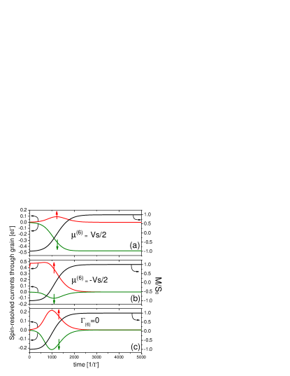
Figure 8: The spin-up and -down currents flowing through the grain and the magnetization of the grain as functions of time when assuming that the chemical potential of region (6) is: (a) $\mu^{(6)}=V_{s}/2$, (b) $\mu^{(6)}=-V_{s}/2$. (c) region (6) is not connected to the grain. The positive direction of current is defined as flowing from lead (4,5) to lead (6). $\theta=0$, $V_{s}=3K_{N}$, $\gamma=0.1$, $T=20$ mK, $S_{0}=100$, $\Delta V_{g}=0$, and other parameters are the same as those in Fig. 3.

We are particularly interested in whether there is truly a pure current flowing through the grain during the reversal in the present device. Therefore, we studied a situation that the grain is initialized at $S_{z}=-S_{0}$ and $I_{c}$ is suddenly switched on to generate a spin bias large enough to drive a switching from $S_{z}=-S_{0}$ to $S_{0}$, then see how the spin-resolved currents and the magnetization evolve with time.

Roughly speaking, if we assume the electrons tunneling through the grain transfer all their angular momenta to the grain, to reverse the grain from $S_{z}=-S_{0}$ to $S_{0}$, there should be at least $4S_{0}$ electrons tunneling through the grain during the reversal. Because the grain is much smaller than region (6), it is safe to expect that the electrons flowing in and out region (6) along with the reversal process will hardly change $\mu^{(6)}$.

According to Fig. 5 (a2), when $V_{s}$ is positive while $S_{z}=-S_{0}$, $\mu^{(6)}$ will saturate at $V_{s}/2$; and when $V_{s}>0$, $S_{z}=S_{0}$, $\mu^{(6)}$ will saturate at $-V_{s}/2$. So in the following we will compare two limits. The first limit assumes that $\mu^{(6)}=V_{s}/2$. The second assumes that $\mu^{(6)}=-V_{s}/2$. These two limits are shown in Figs. 8 (a) and (b), respectively.

Let us first consider the first limit $\mu^{(6)}=V_{s}/2=0.015$ meV. This situation is the same as shown in Fig. 5 (a2), but $V_{s}$ is much larger in magnitude. According to Fig. 8(a), as the magnetization changes from $-S_{0}$ to $S_{0}$, the spin-down current gradually becomes favored and the spin-up current unfavored, which is consistent with the spin selection rules Eq. (17). Remember the configuration of chemical potentials remains unchanged during the reversal as shown in Fig. 5 (a2). As a result, the magnitude of spin-down current will keep growing during the reversal, and even after the magnetization is reversed to $S_{0}$, there will still be a steady spin-down current flowing from lead (6) to lead (4,5). Although not shown in our result, one can expect, for sufficient long time, the spin-down current leaking from region (6) will eventually shift $\mu^{(6)}$ down to $-V_{s}/2$, much like the same situation as shown by Fig. 5 (b2). Then the spin-down current will cease to flow.

The second limit is shown by Fig. 8 (b). At the start, $S_{z}=-S_{0}$, so spin-up current is favored to flow from lead (4,5) to lead (6). As the reversal from $-S_{0}$ to $S_{0}$ goes on, the spin-up current will gradually become unfavored, and drop to zero after the reversal is accomplished. Although the spin-down current is favored when $S_{z}=S_{0}$, the Fermi levels for spin-down electrons on both sides of the grain are the same, so neither the spin-up nor -down current will be flowing after the reversal.

After considering the above two limits, it is natural to expect that a real situation should be between them, i.e., $\mu^{(6)}$ should float gradually from $V_{s}/2$ to $-V_{s}/2$, and there should be a spin-polarized current instead of the anticipated pure spin current flowing through the grain during and after the reversal, until the accumulation or drainage in floating region (6) is accomplished.

The extra charge part of the current is produced along with the electron accumulation or drainage process in region (6). To prove this point, we decouple region (6) completely by letting $\Gamma_{(6)}=0$.Lu et al. (2009) The results are shown in Fig. 8 (c). In this case, the spin-up and down currents are always the same in magnitude and opposite in direction, i.e., there is only a pure spin current flowing. Besides, by integrating the current over time using the data of Fig. 8(c),

$$Q_{\uparrow/\downarrow}=\int_{0}^{\infty}I^{\uparrow/\downarrow}_{(4,5)}\ dt,$$ (30)

we obtain that both the spin-up electrons that tunnel into the grain and spin-down electrons off the grain are $2S_{0}$. This is consistent with the change of $S_{z}$ by $2S_{0}$ during the reversal, where half is from the $2S_{0}$ incoming spin-up electrons and half the $2S_{0}$ outgoing spin-down electrons.

IV.3 Validity of approximation $I^{G}=0$

Because surrounded by insulator, the grain is connected to the leads via the quantum tunneling. The reference 20 of Ref. Kleff et al., 2001 estimates that the tunneling rate for Ref. Guéron et al., 1999 is around $\Gamma=10^{9}$ $\mathrm{s}^{-1}$. According to Fig. 7, where either the magnitude of spin-up or -down current is smaller than $e\Gamma$. Therefore, we estimate the current in and out the grain $I^{G}$ are well smaller than

$$e\Gamma=1.6\times 10^{-19}\mathrm{Coulomb}\times 10^{9}s^{-1}=1.6\times 10^{-10}A$$ (31)

This value is 6 - 7 orders smaller than, e.g., the driven current $I_{c}$ ($\sim 10^{-3}$A) shown in our Fig. 7. So it is valid for us to ignore $I^{G}$ in our numerical calculations, though we explicitly kept it in Eq. 8.

V Summary

In this work, we theoretically studied the magnetization switching and detection of a ferromagnetic nanograin in a non-local spin valve (NLSV) device.

Different from the original experiment,Yang et al. (2008) our nanograin is much smaller in size and at much lower temperatures, thus subjected to strong Coulomb and magnetic blockades. We describe the grain as a Stoner particle, whose ferromagnetism comes from the exchange interactions between itinerant electrons inside it. Because of the ultrasmall size, the one-particle levels inside it are quantized. Because of the ferromagnetism, the level spacings for the majority and minority electrons are unequal.

As shown in Fig. 1(a), the grain is coupled to regions (4)-(6) of the NLSV device via quantum tunneling. Regions (4) and (5), and region (6) can be regarded as two nonmagnetic leads, respectively. In the lead formed by regions (4) and (5), a spin-dependent splitting of chemical potentials (spin bias) is induced by the spin-polarized current $I_{c}$ injected from ferromagnetic injector (1), as shown in Figs. 3(a) and 3(b). The other electrode (6) is floating and connected to region (5) through a voltmeter.

By applying a $I_{c}$ and measure the voltage difference $\Delta V$ between regions (5) and (6), the magnetization of the grain can be read out by the NLSV signal $R_{\mathrm{NLSV}}=\Delta V/I_{c}$. Because of the unequal level spacings for the majority and minority electrons and Coulomb blockade, the NLSV signal in the tunneling regime depends not only on the magnetization of the grain, but also on whether the majority or minority band of the grain is favored to contribute to the electron transport. The results when the minority band is favored are right opposite to when the majority band is favored. In the presence of an angle $\theta$ between the easy-axis of the grain and the spin-quantization direction of the electrode, the NLSV signal is proportional to $\cos\theta$ and vanishes when $\theta=\pi/2$.

By applying $I_{c}$ exceeding a critical value, the magnetization of the grain can be switched reversibly by the spin bias generated by the $I_{c}$. Because of the strong Coulomb and magnetic blockades, the electron flowing between the grain and the electrodes is not possible unless both blockades are lifted, then the angular momenta carried by the flowing electrons can be transferred to the grain. Therefore, the critical value of $I_{c}$ to drive the magnetization switching is determined by: at what gate voltage $V_{g}$ and spin bias $V_{s}$, both the Coulomb and magnetic blockades can be lifted. We also show that the current accompanying the switching may not be a pure spin current, due to the accumulation or drainage of electrons in the floating lead used for the NLSV measurement. A possible solution is to remove the floating lead.

Our numerical evaluations using realistic parameters from the recent NLSVKimura et al. (2006); Yang et al. (2008) and the cobalt grain experimentsGuéron et al. (1999); Deshmukh et al. (2001); Jamet et al. (2001); Thirion et al. (2003) show that it is possible to employ the NLSV device to detect and switch the magnetization of a ferromagnetic nanograin under the present experimental conditions.

VI Acknowledgements

We thank Wei-Qiang Chen, Zhong-Yi Lu, Rong Lv, Chao-Xing Liu, Zhan-Feng Jiang, Rui-Lin Chu, and Wen-Yu Shan for helpful discussions. This work was supported by the Research Grant Council of Hong Kong under Grant No. HKU 704809 and HKU 10/CRF/08.

Appendix A Boundary condition (iii)

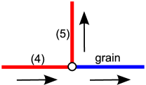
Figure 9: The zoom-in of Fig. 1(b) near interface (4)/(5)/grain. Arrows mark the locally defined positive direction in each region. Three regions meet at the central node. In the local coordinates of (4), the node is at $L$. In the local coordinates of (5), the node is at $0$.

The boundary condition can be found with the help of Fig. 9, which is a zoom-in of Fig. 1(b) near interface (4)/(5)/grain. The positive direction of the locally defined coordinate in each section is marked by arrow. With the help of these arrows, one can write

$$I^{(4)}_{\sigma} = I^{G}_{\sigma}+I^{(5)}_{\sigma},$$ (32)

i.e., the current flowing into the node equals to those flowing out. The current density is related to electrochemical potential by $j_{\sigma}=-(\sigma_{\sigma}/e)\partial_{x}\mu_{\sigma}$. We will take the spin-up component as a example. In (4) and (5), $\sigma_{\uparrow}=\frac{\sigma_{N}}{2}$; and the spin-up current flowing from the node to the grain is defined as $I^{G}_{\uparrow}\equiv I^{G}$. Put these together, one can easily obtain that

$$-A_{\Box}\frac{\sigma_{N}}{2e}\partial_{x}\mu^{(4)}_{\uparrow}(L)=I^{G}-A_{\Box}\frac{\sigma_{N}}{2e}\partial_{x}\mu^{(5)}_{\uparrow}(0).$$ (33)

Similarly, for spin-down $I^{G}_{\downarrow}\equiv-I^{G}$, so

$$-A_{\Box}\frac{\sigma_{N}}{2e}\partial_{x}\mu^{(4)}_{\downarrow}(L)=-I^{G}-A_{\Box}\frac{\sigma_{N}}{2e}\partial_{x}\mu^{(5)}_{\downarrow}(0)$$ (34)

Appendix B The quantum theory of the ferromagnetic nanograin

B.1 Model of ferromagnetic nanograin

In this work, we will describe the ferromagnetic nanograin by using the minimal possible modelCanali and MacDonald (2000); Kleff et al. (2001) proposed to describe the experiment transport spectra through cobalt nanograin.Guéron et al. (1999); Deshmukh et al. (2001) This model was then adopted to discuss spin-polarized current induced relaxation and spin torque.Waintal and Brouwer (2003); Waintal and Parcollet (2005); Parcollet and Waintal (2006) It also provided a starting point to study the Kondo resonance in the STM spectrum of a ferromagnetic cluster on metal surface.Fiete et al. (2002) A more detailed microscopic tight-binding model with exchange interactions and atomic spin-orbit couplings was also proposed,MacDonald and Canali (2001); Cehovin et al. (2002, 2003) to reveal a unified origin of the magnetic anisotropy as well as collective and quasiparticle excitations in the ferromagnetic nanograin. Besides, the Jaynes-Cummings model also reproduced the transport features by considering the interaction between particle-hole excitation and magnon.Michałak et al. (2006)

In this work, we focus on how the collective spin and one-particle excitations of the grain react to the spin bias, therefore the minimal model is adequate for the current topic. The Hamiltonian for the grain and its couplings to nearby leads is given by

$$H_{\mathrm{total}}=H_{G}+H_{\mathrm{lead}}+H_{\mathrm{T}},$$ (35)

where the Hamiltonian for the ferromagnetic grain takes the form,

$$H_{G}=\sum_{i\sigma}\epsilon_{i\sigma}d_{i\sigma}^{{\dagger}}d_{i\sigma}-\frac{J}{2}\mathbf{\hat{S}}\cdot\mathbf{\hat{S}}-\frac{K_{N}}{S_{0}}\hat{S}_{z}^{2}+E_{C}\delta\hat{N}^{2}+V_{g}\delta\hat{N}$$

where the first term stands for the kinetic energy of electrons in the grain, $d_{i\sigma}$ ($d_{i\sigma}^{{\dagger}}$) annihilates (creates) an electron on the one-particle level $i$ in the grain, with energy $\epsilon_{i\sigma}$ and spin $\sigma=\{\uparrow,\downarrow\}$. $\mathbf{\hat{S}}=\sum_{i}\frac{1}{2}\sum_{\sigma\sigma^{\prime}}d_{i\sigma}^{{\dagger}}\overrightarrow{\tau}_{\sigma\sigma^{\prime}}d_{i\sigma^{\prime}}$ is the total angular momentum of the grain electrons, $\overrightarrow{\tau}$ is the vector of Pauli matrices. $J$ is a phenomenological constant depicting the exchange interactions between each pair of electrons in the grain. $\hat{S}_{z}$ is the $z$-component of $\mathbf{\hat{S}}$. $K_{N}$ is the volume-independent anisotropic constant. In this work, we consider that the fluctuation of the electron number ($\sim 1$) is much smaller than than the itinerant electrons $>1000$ already in the grain, so the fluctuation of $K_{N}$ as a function of the electron number is ignored. $\delta N$ is the number of extra electrons added into the grain, compared with a reference electron number $N_{0}$ already in the grain. $E_{C}$ is the charging energy required to add the excess electrons in the grain, which we will see later can be compensated by applying a gate voltage $V_{g}$.

We refer the part where regions (4), (5), and (6) connect the grain as two “leads”, one is from regions (4) and (5) together, and the other from region (6). For convenience, we call them lead (4,5) and lead (6), respectively. The Hamiltonian for the leads takes the form

$$H_{\mathrm{lead}}=\sum_{k,\alpha,\tau}\epsilon_{k\alpha}c_{k\alpha\tau}^{{\dagger}}c_{k\alpha\tau},$$ (37)

where $c_{k\alpha\tau}^{{\dagger}}(c_{k\alpha\tau})$ is the creation (annihilation) operator for a continuous state in lead $\alpha\in\{(4,5),(6)\}$ with energy $\epsilon_{k\alpha}$ and spin $\tau\in\{+,-\}$. The tunneling between the grain and the leads is described by

$$H_{\mathrm{T}} = \sum_{k,\alpha,i}V_{k\alpha}[(\cos\frac{\theta_{\alpha}}{2}c_{k\alpha+}^{{\dagger}}-\sin\frac{\theta_{\alpha}}{2}c_{k\alpha-}^{{\dagger}})d_{i\uparrow}$$

$$\ \ \ \ \ \ \ \ \ +(\sin\frac{\theta_{\alpha}}{2}c_{k\alpha+}^{{\dagger}}+\cos\frac{\theta_{\alpha}}{2}c_{k\alpha-}^{{\dagger}})d_{i\downarrow}]+H.c.,$$

where $\theta_{\alpha}$ is the angle between the easy axis of the grain and the spin-quantization direction of lead $\alpha$. For simplicity, we set the easy-axis of the grain as $z$-axis and assume that $\theta_{(6)}=0$ and $\theta_{(4,5)}=\theta\in[0,\pi/2]$, as shown in Fig. 4. In the following, we denote $\mu_{+/-}^{(4)}=\mu_{\uparrow/\downarrow}^{(4)}$ when $\theta_{(4,5)}=0$ for simplicity.

B.2 Ground branch $|N_{0},S_{0},S_{z}\rangle$ of the grain and possible excitations

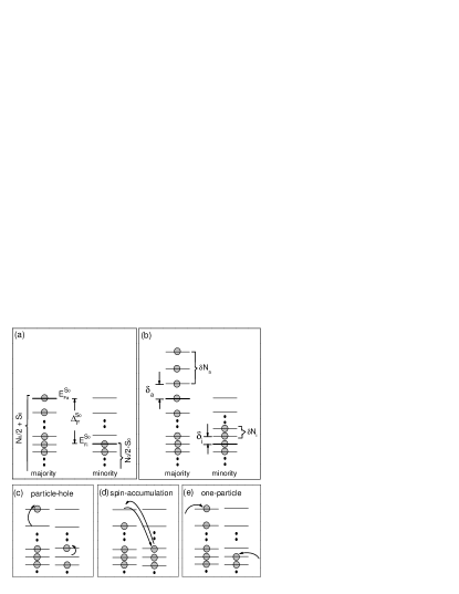
Figure 10: The filling of one-particle levels in the majority and minority bands of the grain with (a) $N_{0}$ electrons, and (b) $N_{0}+\delta N$ electrons, where $\delta N=\delta N_{a}+\delta N_{i}$, and $\delta N_{a}$ and $\delta N_{i}$ are the excess electrons added to the majority and minority band, respectively. For the ground branch with $N_{0}$ electrons in the grain, the magnitude of the angular momentum $S=S_{0}$. $E_{Fa}^{S_{0}}$, and $E_{Fi}^{S_{0}}$ are the highest occupied levels of the majority and minority bands for the ground branch for $N=N_{0}$ and $S=S_{0}$. $\delta_{a}$ and $\delta_{i}$ is the level spacings near the $E_{Fa}^{S_{0}}$ and $E_{Fi}^{S_{0}}$, respectively. (c) The particle-hole excitations, with excitation energy $\sim\delta_{i},\delta_{a}>1$meV. (d) The spin-accumulation excitations, with excitation energy $\sim J\sim 2$meV. These two excitations are high-energy excitations, with the excitation energy larger than the spin bias $V_{s}$, thus can not be excited and will be omitted. Note that according to Fig. 3, $V_{s}\sim 0.1$ meV. (e) One-particle excitations that changes the electron number by one. It can add extra electrons to the majority or minority band. By tuning the gate voltage, its excitation energy can be minimized down to $\sim K_{N}\sim 0.01$meV, which is smaller than the spin bias $V_{s}\sim 0.1$meV. Then, one-particle excitations is the only possible excitation for the present device and parameters.

The eigen states of $H_{G}$ are labeled by $|\{n_{i}\},S,S_{z}\rangle$, where $\{n_{i}\}$ denote the occupation on each level in the grain, $S$ and $S_{z}$ are, respectively, the quantum numbers for the magnitude of $\mathbf{\hat{S}}$ and $\hat{S}_{z}$. Because of the low experimental temperature (as low as 20 mK) and the large Coulomb repulsion $E_{C}$ ($>30$ meV),Guéron et al. (1999) the charge fluctuation and particle-hole excitations [Fig. 10 (c)] are suppressed hence it is reasonable to assume that the electrons in the grain compactly occupy all the lowest available levels. These states are denoted as $|N,S,S_{z}\rangle$, where $N=\sum_{i}n_{i}$ is the total electron number in the grain.

When there is $N=N_{0}$ electrons in the grain, the competition between the kinetic energy and the $J$ term will force $N_{0}/2+S_{0}$ electrons (the majority band) to orient anti-parallel with the rest $N_{0}/2-S_{0}$ electrons (the minority band), leading to a nonzero magnitude of angular momentum $S=S_{0}$ at the ground states(Stoner instability), as shown in Figs. 4 and 10 (a). This overall ground branch is denoted as $|N_{0},S_{0},S_{z}\rangle$, where $S_{z}\in[-S_{0},S_{0}]$. The $(2S_{0}+1)$-fold degeneracy of the overall ground branch is lifted by the anisotropy, with two degenerate ground states $|N_{0},S_{0},\pm S_{0}\rangle$.

There are three kinds of basic excitations from the ground branches $|N_{0},S_{0},S_{z}\rangle$, as shown in Fig. 10(c), (d), and (e). The particle-hole excitation destroys the compact occupation of the one-particle levels, while does not change $N$, $S$, and $S_{z}$. The spin-accumulation excitation changes $S$ by moving electron between the majority and minority bands, while does not change $N_{0}$ and $S_{z}$. The one-particle excitation changes $N$ by adding or removing electrons, which also leads to changes in $S$ and $S_{z}$.

Generally, the excited energy from $|N_{0},S_{0},S_{z}\rangle$ to $|N_{0}+\delta N,S_{0}+\delta S,S_{z}+\delta S_{z}\rangle$ can be found with the help of Figs. 10(a) and (b) as (using the relations $\delta N=\delta N_{a}+\delta N_{i}$ and $\delta S=(\delta N_{a}-\delta N_{i}$)/2),Canali and MacDonald (2000); Kleff and von Delft (2002)

$$\delta E(\delta N,\delta S,\delta S_{z})$$ (39)

$$\equiv E_{|N_{0}+\delta N,S_{0}+\delta S,S_{z}+\delta S_{z}\rangle}-E_{|N_{0},S_{0},S_{z}\rangle}$$

$$= (\delta N)^{2}[E_{C}+\frac{1}{8}\delta_{a}+\frac{1}{8}\delta_{i}]+\delta N[\overline{E}_{F}^{S_{0}}+\frac{1}{4}\delta_{a}+\frac{1}{4}\delta_{i}+V_{g}]$$

$$+ (\delta S)^{2}[\frac{\delta_{a}}{2}+\frac{\delta_{i}}{2}-\frac{J}{2}]+\delta S[\frac{\delta_{a}}{2}-\frac{\delta_{i}}{2}+\Delta_{F}^{S_{0}}-J(S_{0}+\frac{1}{2})]$$

$$+ \delta N\delta S[\frac{1}{2}\delta_{a}-\frac{1}{2}\delta_{i}]-\frac{K_{N}}{S_{0}}(2S_{z}\delta S_{z}+\delta S_{z}^{2}),$$

where the definitions of parameters are given in Fig. 10 and $\overline{E}_{F}^{S_{0}}=(E_{Fa}^{S_{0}}+E_{Fi}^{S_{0}})/2$.

Table 1: Parameters for a $S_{0}=1000$ grain. All energies are in meV.Canali and MacDonald (2000); Kleff and von Delft (2002) $E_{C}$, $S_{0}$, $K_{N}$ are estimated by experiments,Guéron et al. (1999); Deshmukh et al. (2001); Jamet et al. (2001); Thirion et al. (2003) $\delta_{a}$, $\delta_{i}$, $\Delta_{F}^{S_{0}}$ are from the band calculations.Papaconstantopoulos (1986) According to Eq. (39), $\overline{E}_{F}^{S_{0}}$ can be absorbed into $V_{g}$, thus is set to 0 for convenience. $\mu^{(5)}(\infty)$ is the energy zero point throughout the paper.

$E_{C}$	$K_{N}$	$\delta_{a}$	$\delta_{i}$	$\Delta_{F}^{S_{0}}$	$\overline{E}_{F}^{S_{0}}$	$\mu^{(5)}(\infty)$
30	0.01	4.61	1.19	2000	0	0

We will adopt a set of parameters for a grain with $S_{0}=1000$, as given in Tab. 1. The theoretical calculationsCanali and MacDonald (2000); Kleff et al. (2001); Kleff and von Delft (2002) based on these parameters are consistent with most features observed in the experimental transport spectra.Guéron et al. (1999); Deshmukh et al. (2001) With these parameters, the value of $J$ can be deduced using a saddle point analysis as follows.

B.3 Range of $J$ for a stable $S_{0}$ by saddle-point analysis

Above we just assume that $S=S_{0}$ when there are $N=N_{0}$ electrons in the grain. Since $S_{0}$ originates from the competition between the $J$ term and the kinetic energy, its value should be calculated for the given values of $J$ and $\delta_{a,i}$. However, since we already know $S_{0}\sim 1000$ from the experiments,Guéron et al. (1999); Deshmukh et al. (2001); Jamet et al. (2001); Thirion et al. (2003) and $\delta_{a,i}$ from the band calculation,Papaconstantopoulos (1986) we will use these data to conversely deduce the value of $J$, then generate other information (e.g., one-particle excitations) at the proximity of the deduced $J$, much like a saddle-point analysis.

The stability of the branch $|N=N_{0},S=S_{0}\rangle$ requires that its energy should be at least locally minimal compared to the states $|N=N_{0},S=S_{0}\pm 1\rangle$, i.e.,

$$\delta E(\delta N=0,\delta S=+1) = \delta_{a}+\Delta_{F}^{S_{0}}-J(S_{0}+1)\geq 0,$$

$$\delta E(\delta N=0,\delta S=-1) = \delta_{i}-\Delta_{F}^{S_{0}}+JS_{0}\geq 0,$$ (40)

where we have used Eq. (39) and ignored the anisotropy term because $K_{N}$ is much smaller than other energies. In other words, Eq. (B.3) leads to that, for $J$ belongs to the range

$$\frac{\Delta_{F}^{S_{0}}-\delta_{i}}{S_{0}}\leq J\leq\frac{\Delta_{F}^{S_{0}}+\delta_{a}}{S_{0}+1},$$ (41)

the grain will adopt a stable $S=S_{0}$ when there are $N_{0}$ electrons in the grain. Once $J$ exceeds this range, the overall ground branch will evolve to adopt a smaller or larger $S=S_{0}^{\prime}=S_{0}\mp 1$, then Eq. (41) still holds for the new $S_{0}^{\prime}$ (note that $\Delta_{F}^{S_{0}\pm 1}=\Delta_{F}^{S_{0}}\pm\delta_{a}\mp\delta_{i}$).

B.4 One-particle excitations to the branches $|N_{0}+1,S_{0}\pm 1/2,S_{z}\rangle$

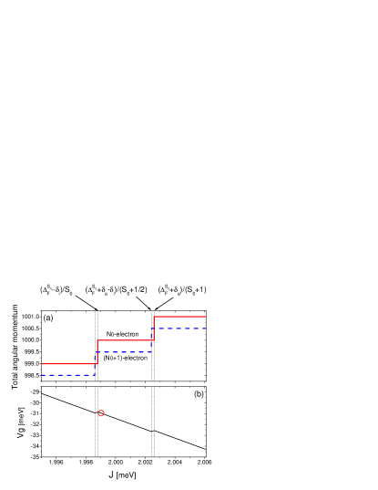
Figure 11: (a) Total angular momenta for the ground branches of the grain with $N_{0}$ and $N_{0}+1$ electrons, respectively. (b) Along the zigzag line of $(J,V_{g})$, the $N_{0}$- and $(N_{0}+1)$-electron ground branches are nearly degenerate. The parameters are listed in Table 1.

The excitation energies for the particle-hole excitation shown in Fig. 10 (c) and spin-accumulation excitation shown in Fig. 10 (d) are of the order of $\delta_{a/i}$ and $J$, respectively.Canali and MacDonald (2000); Kleff and von Delft (2002); Parcollet and Waintal (2006) According to the parameters for $S_{0}=1000$ shown in Tab. 1, these excitations are of meV, much larger than the $V_{s}\sim 0.05$ meV estimated in Fig. 3, thus will be excluded. In the following, we will only consider the one-particle excitation from the $N_{0}$ to $N_{0}+1$ electrons, as shown by Fig. 10 (e), i.e., adding excess electrons to the grain.

Again, because $E_{C}\gg k_{B}T$, the gate voltage in this work is restricted so that one and only one excess electron ($\delta N=1$) can be added into the grain. Depending on this excess electron being added to the majority or minority band, the magnitude of the angular momentum could change to $S=S_{0}+1/2$ or $S_{0}-1/2$, respectively. With the help of Eqs. (39) and (41), we find that, when

$$\frac{\Delta_{F}^{S_{0}}-\delta_{i}}{S_{0}}\leq J\leq\frac{\Delta_{F}^{S_{0}}+\delta_{a}-\delta_{i}}{S_{0}+1/2},$$ (42)

the $N_{0}+1$-electron ground branch will adopt $S=S_{0}-1/2$, and the required transition energies from $|N_{0},S_{0},S_{z}\rangle$ are

$$E_{|N_{0}+1,S_{0}-\frac{1}{2},S_{z}\pm\frac{1}{2}\rangle}-E_{|N_{0},S_{0},S_{z}\rangle}$$

$$= \delta_{i}+V_{g}+E_{C}+E_{Fi}^{S_{0}}+\frac{J}{2}(S_{0}+\frac{1}{4})-\frac{K_{N}}{S_{0}}(\frac{1}{4}\pm S_{z}).$$

On the contrary, when

$$\frac{\Delta_{F}^{S_{0}}+\delta_{a}-\delta_{i}}{S_{0}+1/2}\leq J\leq\frac{\Delta_{F}^{S_{0}}+\delta_{a}}{S_{0}+1},$$ (44)

the $N_{0}+1$-electron ground branch will adopt $S=S_{0}+1/2$, and the required transition energies from $|N_{0},S_{0},S_{z}\rangle$ are

$$E_{|N_{0}+1,S_{0}+\frac{1}{2},S_{z}\pm\frac{1}{2}\rangle}-E_{|N_{0},S_{0},S_{z}\rangle}$$

$$= \delta_{a}+V_{g}+E_{C}+E_{Fa}^{S_{0}}-\frac{J}{2}(S_{0}+\frac{3}{4})-\frac{K_{N}}{S_{0}}(\frac{1}{4}\pm S_{z}).$$

To summarize the above saddle-point analysis, the angular momenta of $N_{0}$- and $(N_{0}+1)$-electron ground branches as a function of $J$ are shown in Fig. 11(a), in which the arrows mark the ranges indicated by Eqs. (41), (42) and (44).

According to Fig. 11(a), for most value of $J$, $S$ of the $(N_{0}+1)$-electron branch is $1/2$ smaller than that of the $N_{0}$-electron branch. This is a direct results of $\delta_{i}<\delta_{a}$. Although $J$ is not a tunable quantity, Fig. 11(a) implies that in reality the excess electron is far more likely to occupy the minority band than the majority band, which is also consistent with the previous literatures.Canali and MacDonald (2000); Waintal and Parcollet (2005) Therefore, in the following we will mainly consider the one-particle excitations between the ground branches $|N_{0},S_{0},S_{z}\rangle$ and $|N_{0}+1,S_{0}-1/2,S_{z}\rangle$.

B.5 States used for numerical simulations

Remember we have set $\mu^{(5)}(\infty)$ as the energy zero point. With respect to $\mu^{(5)}(\infty)$, we can always choose suitable $V_{g}$ in Eqs. (B.4) and (B.4) to compensate $E_{C}$ and other energies, so that the ground-branches with $N_{0}$ and $N_{0}+1$ electrons can be tuned to be nearly degenerate. These $V_{g}$ as a function of $J$ are shown in Fig. 11(b). For instance, in Eq. (B.4), by choosing $V_{g}=-\delta_{i}-E_{C}-E_{Fi}^{S_{0}}-J(S_{0}+1/4)/2+K_{N}/4S_{0}$, one obtains

$$E_{|N_{0}+1,S_{0}-\frac{1}{2},S_{z}\pm\frac{1}{2}\rangle}-E_{|N_{0},S_{0},S_{z}\rangle}=\mp\frac{K_{N}}{S_{0}}S_{z}.$$ (46)

In this context, the energy required to add an electron from lead (4,5) into the grain is related to only the magnetization of the grain. According to Eq. (46), the spectrum width of $E_{|N_{0}+1,S_{0}-\frac{1}{2},S_{z}\pm\frac{1}{2}\rangle}-E_{|N_{0},S_{0},S_{z}\rangle}$ is $2K_{N}$ for all the possible $S_{z}\in[-S_{0},S_{0}]$. This value is the key to determine the critical $I_{c}$ in the Sec. IV.1.

Experimentally, it is easy to find the suitable $V_{g}$ at which the ground-branches with $N_{0}$ and $N_{0}+1$ electrons are nearly-degenerate, as in the usual transport experiments.Guéron et al. (1999); Deshmukh et al. (2001) For example, one just apply a small charge bias voltage $>2K_{N}$ between lead (4,5) and lead (6), and measure the current through the grain while scanning $V_{g}$, like a usual source-gate-drain measurement. Because of the Coulomb blockade, the grain can not conduct electrons unless the $N_{0}$- and $(N_{0}+1)$-electron ground-branches are degenerate. Therefore, the nearly-degenerate situation is find as: at which $V_{g}$, the grain is conducting under a small charge bias voltage between (4) and (6).

Based on the above analysis and discussions from Appendixes B.2-B.5, in the following, we will consider mainly the one-particle excitations from the branches $|N_{0},S_{0},S_{z}\rangle$ to $|N_{0}+1,S_{0}-1/2,S_{z}\rangle$ and when their energies are nearly degenerate. Specifically, we will choose a set of $(J,V_{g})$ marked by the circle in Fig. 11(b) for our numerical simulations, where $J=\Delta_{F}^{S_{0}}/(S_{0}+1/2)$, and $V_{g}=-\delta_{i}-E_{C}-E_{Fi}^{S_{0}}-J(S_{0}+1/4)/2+K_{N}/4S_{0}+\Delta V_{g}$, $\Delta V_{g}$ is a small variation of the gate voltage that drives the grain away from the nearly-degenerate point of $N_{0}$- and $(N_{0}+1)$-electron ground branches.

Appendix C Validity of Rate equations

Although the rate equations formalism is widely employed for the mesoscopic systems weakly coupled to the electrodes, its validity deserves some discussion.Beenakker (1991); von Delft and Ralph (2001)

In the previous works by Waintal et al,Waintal and Parcollet (2005); Parcollet and Waintal (2006) the intrinsic spin relaxation is considered in terms of coupling to a bosonic bath. We do not consider this effect for two reasons: (i) According to Eq. (3) of Ref. Waintal and Parcollet, 2005, the intrinsic relaxation will lead to a term similar to the Gilbert damping, which tends to relax the grain to one of its two degenerate maximally magnetized ground states, e.g., $|N_{0},S_{0},-S_{0}\rangle$ or $|N_{0},S_{0},S_{0}\rangle$. In the following, we will mainly discuss how to use the NLSV signal to read out the magnetization of the grain (Sec. III), which already limits the discussion to these maximally magnetized states. Therefore, the results in Sec. III will be qualitatively unaffected by the intrinsic relaxation. (ii) For the spin bias -induced magnetization switching discussed in Sec. IV, the results are only valid when the coupling between the grain and the lead is dominant and much smaller in time scale than the intrinsic relaxation. On the other hand, the Born and Markoff approximations enforce that $\Gamma$ is much smaller than $k_{B}T$ (bath temperature) and the energy difference between many-body states in the grain. These two requirements confine the validity range of $\Gamma$ in this work.

Besides, the particle-hole excitation terms in Eq. (10) of Ref. Kleff and von Delft, 2002 are also absent in this work, because the energy scale of these excitations are of the order $\delta_{a},\delta_{i}>$ 1meV, which already one order larger than the spin bias ($V_{s}\sim 0.1$meV) that can be generated according to Fig. 3.

References

- Slonczewski (1996) J. C. Slonczewski, J. Magn. Magn. Mater. 159, 1 (1996).
- Berger (1996) L. Berger, Phys. Rev. B 54, 9353 (1996).
- Tsoi et al. (1998) M. Tsoi, A. G. M. Jansen, J. Bass, W. C. Chiang, M. Seck, V. Tsoi, and P. Wyder, Phys. Rev. Lett. 80, 4281 (1998).
- Myers et al. (1999) E. B. Myers, D. C. Ralph, J. A. Katine, R. N. Louie, and R. A. Buhrman, Science 285, 867 (1999).
- Sun (1999) J. Z. Sun, J. Magn. Magn. Mater. 202, 157 (1999).
- Katine et al. (2000) J. A. Katine, F. J. Albert, R. A. Buhrman, E. B. Myers, and D. C. Ralph, Phys. Rev. Lett. 84, 3149 (2000).
- Jiang et al. (2004) Y. Jiang, S. Abe, T. Ochiai, T. Nozaki, A. Hirohata, N. Tezuka, and K. Inomata, Phys. Rev. Lett. 92, 167204 (2004).
- Guéron et al. (1999) S. Guéron, M. M. Deshmukh, E. B. Myers, and D. C. Ralph, Phys. Rev. Lett. 83, 4148 (1999).
- Deshmukh et al. (2001) M. M. Deshmukh, S. Kleff, S. Guéron, E. Bonet, A. N. Pasupathy, J. von Delft, and D. C. Ralph, Phys. Rev. Lett. 87, 226801 (2001).
- Jamet et al. (2001) M. Jamet, W. Wernsdorfer, C. Thirion, D. Mailly, V. Dupuis, P. Mélinon, and A. Pérez, Phys. Rev. Lett. 86, 4676 (2001).
- Thirion et al. (2003) C. Thirion, W. Wernsdorfer, and D. Mailly, Nat. Mater. 2, 524 (2003).
- Inoue and Brataas (2004) J. I. Inoue and A. Brataas, Phys. Rev. B 70, 140406(R) (2004).
- Braun et al. (2004) M. Braun, J. König, and J. Martinek, Phys. Rev. B 70, 195345 (2004).
- Wetzels et al. (2005) W. Wetzels, G. E. W. Bauer, and M. Grifoni, Phys. Rev. B 72, 020407(R) (2005).
- Jalil and Tan (2005) M. B. A. Jalil and S. G. Tan, Phys. Rev. B 72, 214417 (2005).
- Waintal and Parcollet (2005) X. Waintal and O. Parcollet, Phys. Rev. Lett. 94, 247206 (2005).
- Parcollet and Waintal (2006) O. Parcollet and X. Waintal, Phys. Rev. B 73, 144420 (2006).
- Fernández-Rossier and Aguado (2007) J. Fernández-Rossier and R. Aguado, Phys. Rev. Lett. 98, 106805 (2007).
- Wang and Sun (2007) X. R. Wang and Z. Z. Sun, Phys. Rev. Lett. 98, 077201 (2007).
- Lu and Shen (2008) H.-Z. Lu and S.-Q. Shen, Phys. Rev. B 77, 235309 (2008).
- Lu et al. (2009) H.-Z. Lu, B. Zhou, and S.-Q. Shen, Phys. Rev. B 79, 174419 (2009).
- Chen et al. (2006) T. Y. Chen, S. X. Huang, C. L. Chien, and M. D. Stiles, Phys. Rev. Lett. 96, 207203 (2006).
- Krause et al. (2007) S. Krause, L. Berbil-Bautista, G. Herzog, M. Bode, and R. Wiesendanger, Science 317, 1537 (2007).
- Wang et al. (2008) X. J. Wang, H. Zou, and Y. Ji, Appl. Phys. Lett. 93, 162501 (2008).
- Garzon et al. (2008) S. Garzon, L. Ye, R. A. Webb, T. M. Crawford, M. Covington, and S. Kaka, Phys. Rev. B 78, 180401(R) (2008).
- Ralph and Stiles (2008) D. Ralph and M. D. Stiles, J. Magn. Magn. Mater. 320, 1190 (2008).
- Johnson and Silsbee (1985) M. Johnson and R. H. Silsbee, Phys. Rev. Lett. 55, 1790 (1985).
- Filip et al. (2000) A. T. Filip, B. H. Hoving, F. J. Jedema, B. J. van Wees, B. Dutta, and S. Borghs, Phys. Rev. B 62, 9996 (2000).
- Jedema et al. (2001) F. J. Jedema, A. T. Filip, and B. J. van Wees, Nature(London) 410, 345 (2001).
- Valenzuela and Tinkham (2004) S. O. Valenzuela and M. Tinkham, Appl. Phys. Lett. 85, 5914 (2004).
- Ji et al. (2004) Y. Ji, A. Hoffmann, J. S. Jiang, and S. D. Bader, Appl. Phys. Lett. 85, 6218 (2004).
- Beckmann et al. (2004) D. Beckmann, H. B.Weber, and H. v. Lhneysen, Phys. Rev. Lett. 93, 197003 (2004).
- Kimura et al. (2004) T. Kimura, J. Hamrle, Y. Otani, K. Tsukagoshi, and Y. Aoyagi, Appl. Phys. Lett. 85, 3501 (2004).
- Garzon et al. (2005) S. Garzon, I. Zutic, and R. A. Webb, Phys. Rev. Lett. 94, 176601 (2005).
- Brataas et al. (2006) A. Brataas, G. E. Bauer, and P. J. Kelly, Phys. Rep. 427, 157 (2006).
- Kimura et al. (2006) T. Kimura, Y. Otani, and J. Hamrle, Phys. Rev. Lett. 96, 037201 (2006).
- Yang et al. (2008) T. Yang, T. Kimura, and Y. Otani, Nature Phys. 4, 851 (2008).
- van Son et al. (1987) P. C. van Son, H. van Kempen, and P. Wyder, Phys. Rev. Lett. 58, 2271 (1987).
- Valet and Fert (1993) T. Valet and A. Fert, Phys. Rev. B 48, 7099 (1993).
- Hershfield and Zhao (1997) S. Hershfield and H. L. Zhao, Phys. Rev. B 56, 3296 (1997).
- Jedema et al. (2003) F. J. Jedema, M. S. Nijboer, A. T. Filip, and B. J. van Wees, Phys. Rev. B 67, 085319 (2003).
- Takahashi and Maekawa (2003) S. Takahashi and S. Maekawa, Phys. Rev. B 67, 052409 (2003).
- Sun (2000) J. Z. Sun, Phys. Rev. B 62, 570 (2000).
- Waintal and Brouwer (2003) X. Waintal and P. W. Brouwer, Phys. Rev. Lett. 91, 247201 (2003).
- Canali and MacDonald (2000) C. M. Canali and A. H. MacDonald, Phys. Rev. Lett. 85, 5623 (2000).
- Kleff et al. (2001) S. Kleff, J. von Delft, M. M. Deshmukh, and D. C. Ralph, Phys. Rev. B 64, 220401(R) (2001).
- Wang et al. (2004) D.-K. Wang, Q.-F. Sun, and H. Guo, Phys. Rev. B 69, 205312 (2004).
- Sun et al. (2008) Q.-F. Sun, Y. Xing, and S. Q. Shen, Phys. Rev. B 77, 195313 (2008).
- Xing et al. (2008) Y. Xing, Q.-F. Sun, and J. Wang, Appl. Phys. Lett. 93, 142107 (2008).
- Stefanucci et al. (2008) G. Stefanucci, E. Perfetto, and M. Cini, Phys. Rev. B 78, 075425 (2008).
- Bass and Jr (2007) J. Bass and W. P. P. Jr, J. Phys.: Condens. Matter 19, 183201 (2007).
- Beenakker (1991) C. W. J. Beenakker, Phys. Rev. B 44, 1646 (1991).
- Blum (1996) K. Blum, Density Matrix Theory and Applications (Plenum Press, New York, 1996).
- von Delft and Ralph (2001) J. von Delft and D. C. Ralph, Phys. Rep. 345, 61 (2001).
- Kimura et al. (2007) T. Kimura, Y. Otani, and P. M. Levy, Phys. Rev. Lett. 99, 166601 (2007).
- Fiete et al. (2002) G. A. Fiete, G. Zarand, B. I. Halperin, and Y. Oreg, Phys. Rev. B 66, 024431 (2002).
- MacDonald and Canali (2001) A. H. MacDonald and C. M. Canali, Solid State Commun. 119, 353 (2001).
- Cehovin et al. (2002) A. Cehovin, C. M. Canali, and A. H. MacDonald, Phys. Rev. B 66, 094430 (2002).
- Cehovin et al. (2003) A. Cehovin, C. M. Canali, and A. H. MacDonald, Phys. Rev. B 68, 014423 (2003).
- Michałak et al. (2006) L. Michałak, C. M. Canali, and V. G. Benza, Phys. Rev. Lett. 97, 096804 (2006).
- Kleff and von Delft (2002) S. Kleff and J. von Delft, Phys. Rev. B 65, 214421 (2002).
- Papaconstantopoulos (1986) D. A. Papaconstantopoulos, Handbook of the Band Structure of Elemental Solids (Plenum, New York, 1986).