Raptor Codes Based Distributed Storage Algorithms for Wireless Sensor Networks

Abstract

We consider a distributed storage problem in a large-scale wireless sensor network with $n$ nodes among which $k$ acquire (sense) independent data. The goal is to disseminate the acquired information throughout the network so that each of the $n$ sensors stores one possibly coded packet and the original $k$ data packets can be recovered later in a computationally simple way from any $(1+\epsilon)k$ of nodes for some small $\epsilon>0$. We propose two Raptor codes based distributed storage algorithms for solving this problem. In the first algorithm, all the sensors have the knowledge of $n$ and $k$. In the second one, we assume that no sensor has such global information.

I Introduction

We consider a distributed storage problem in a large-scale wireless sensor network with $n$ nodes among which $k$ sensor nodes acquire (sense) independent data. Since sensors are usually vulnerable due to limited energy and hostile environment, it is desirable to disseminate the acquired information throughout the network so that each of the $n$ sensors stores one possibly coded packet and the original $k$ source packets can be recovered later in a computationally simple way from any $(1+\epsilon)k$ of nodes for some small $\epsilon>0$. No sensor knows locations of any other sensors except for their own neighbors, and they do not maintain any routing information (e.g., routing tables or network topology).

Algorithms that solve such problems using coding in a centralized way are well known and understood. In a sensor network, however, this is much more difficult, since we need to find a strategy to distribute the information from multiple sources throughout the network so that each sensor admits desired statistics of data. In [7], Lin et al. proposed an algorithm that uses random walks with traps to disseminate the source packets in a wireless sensor network. To achieve desired code degree distribution, they employed the Metropolis algorithm to specify transition probabilities of the random walks. While the proposed methods in [7] are promising, the knowledge of the total number of sensors $n$ and sources $k$ are required. Another type of global information, the maximum node degree (i.e., the maximum number of neighbors) of the graph, is also required to perform the Metropolis algorithm. Nevertheless, for a large-scale sensor network, these types of global information may not be easy to obtain by each individual sensor, especially when there is a possibility of change of topology.

In [1, 2], we proposed Luby Transform (LT) codes based distributed storage algorithms for large-scale wireless sensor networks to overcome these difficulties. In this paper, we extend this work to Raptor codes and demonstrate their performance. Particularly, we propose two new decentralized algorithms, Raptor Code Distributed Storage (RCDS-I) and (RCDS-II), that distribute information sensed by k source nodes to n nodes for storage based on Raptor codes. In RCDS-I, each node has limited global information; while in RCDS-II, no global information is required. We compute the computational encoding and decoding complexity of these algorithms as well as evaluate their performance by simulation.

II Wireless Sensor Networks and Fountain Codes

II-A Network Model

Suppose that the wireless sensor network consists of $n$ nodes that are uniformly distributed at random in a region $\mathcal{A}=[L,L]^{2}$. Among these $n$ nodes, there are $k$ source nodes that have information to be disseminated throughout the network for storage. These $k$ nodes are uniformly and independently chosen at random among the $n$ nodes. Usually, the fraction of source nodes.

We assume that no node has knowledge about the locations of other nodes and no routing table is maintained, and thus that the algorithm proposed in [4] cannot be applied. Moreover, besides the neighbor nodes, we assume that each node has limited or no knowledge of global information. The limited global information refers to the total number of nodes $n$, and the total number of sources $k$. Any further global information, for example, the maximal number of neighbors in the network, is not available. Hence, the algorithms proposed in [7, 6, 5] are not applicable.

Definition 1

(Node Degree) Consider a graph $G=(V,E)$, where $V$ and $E$ denote the set of nodes and links, respectively. Given $u,v\in V$, we say $u$ and $v$ are adjacent (or $u$ is adjacent to $v$, and vice versa) if there exists a link between $u$ and $v$, i.e., $(u,v)\in E$. In this case, we also say that $u$ and $v$ are neighbors. Denote by $\mathcal{N}(u)$ the set of neighbors of a node $u$. The number of neighbors of a node $u$ is called the node degree of $u$, and denoted by $d_{n}(u)$, i.e., $|\mathcal{N}(u)|=d_{n}(u)$. The mean degree of a graph $G$ is then given by $\mu=\frac{1}{|V|}\sum_{u\in G}d_{n}(u)$.

II-B Fountain Codes and Raptor Codes

Definition 2

(Code Degree) For Fountain codes, the number of source blocks used to generate an encoded output $y$ is called the code degree of $y$, and denoted by $d_{c}(y)$. The code degree distribution $\Omega(d)$ is the probability distribution of $d_{c}(y)$.

For $k$ source blocks $\{x_{1},x_{2},\ldots,x_{k}\}$ and a probability distribution $\Omega(d)$ with $1\leq d\leq k$, a Fountain code with parameters $(k,\Omega)$ is a potentially limitless stream of output blocks $\{y_{1},y_{2},...\}$. Each output block is obtained by XORing $d$ randomly and independently chosen source blocks, where $d$ is drawn from a degree distribution $\Omega(d)$. This is illustrated in Fig. 1.

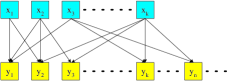
Figure 1: The encoding operations of Fountain codes: each output is obtained by XORing $d$ source blocks chosen uniformly and independently at random from $k$ source inputs, where $d$ is drawn according to a probability distribution $\Omega(d)$.

Raptor codes are a class of Fountain codes with linear encoding and decoding complexity [11, 10]. The key idea of Raptor codes is to relax the condition that all input blocks need to be recovered. If an LT code needs to recover only a constant fraction of its input blocks, its decoding complexity is $O(k)$, i.e., linear time decoding. Then, we can recover all input blocks by concatenating a traditional erasure correcting code with an LT code. This is called pre-coding in Raptor codes, and can be accomplished by a modern block code such as LDPC codes. This process is illustrated in Fig. 2.

The pre-code $\mathcal{C}_{m}$ used in this paper is the randomized LDPC (Low-Density Parity-Check) code that is studied as one type of pre-code in [10]. In this randomized LDPC code, we have $k$ source blocks and $m$ pre-coding output blocks. Each source block chooses $d$ pre-coding output blocks uniformly independently at random, where $d$ is drawn from a distribution $\Omega_{L}(d)$. Each pre-coding output blocks combines the “incoming” source blocks and obtain the encoded output.

The code degree distribution $\Omega_{r}(i)$ of Raptor codes for LT coding is a modification of the Ideal Soliton distribution and given by

$$\Omega_{r}(i)=\left\{\begin{array}[]{ll}\displaystyle\frac{\rho}{1+\rho},&i=1,\\ \displaystyle\frac{1}{i(i-1)(1+\rho)},&i=2,...,D,\\ \displaystyle\frac{1}{D(1+\rho)},&i=D+1,\end{array}\right.$$ (1)

where $D=\lceil 4(1+\epsilon)\epsilon\rceil$ and $\rho=(\epsilon/2)+(\epsilon/2)^{2}$.

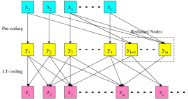
Figure 2: The encoding operations of raptor codes: $k$ source blocks are first encoded to $m$ pre-coding output blocks by LDPC coding, and then the final encoded output blocks are obtained by applying LT codes with these $m$ pre-coding output blocks with degree distribution $\Omega_{r}(d)$.

The following result provides the performance of the Raptor codes [11, 10].

Lemma 1 (Shokrollahi [11, 10])

Let $R_{0}=(1+\epsilon/2)/(1+\epsilon)$, and $\mathcal{C}_{m}$ be the family of codes of rate $R_{0}$. Then, the Raptor code with pre-code $\mathcal{C}_{m}$ and LT codes with degree distribution $\Omega_{r}(d)$ has a linear time encoding algorithm. With $(1+\epsilon)k$ encoded output blocks, the BP decoding algorithm has a linear time complexity. More precisely, the average number of operations to produce an output symbol is $O(\log(1/\epsilon))$, and the average number of operations to recover the $k$ source symbols is $O(k\log(1/\epsilon))$.

III Raptor Codes Based Distributed Storage (RCDS) Algorithms

As shown in [7, 1], distributed LT codes are relatively simple to implement. Raptor codes take the advantage of LT codes to decode a major fraction of $k$ source packets within linear complexity, and use another error correcting code to decode the remaining minor fraction also within linear complexity by concatenating such an error correcting code and LT code together [10].

Nevertheless, it is not trivial to achieve this encoding mechanism in a distributed manner. In this section, we propose two algorithms for distributed storage based on Raptor codes. The first is called RCDS-I, in which each node has knowledge of limited global information. The second is called RCDS-II, which is a fully distributed algorithm and does not require any global information.

III-A With Limited Global Information—RCDS-I

In RCDS-I, we assume that each node in the network knows the value of $k$—the number of sources, and the value of $n$—the number of nodes. We use simple random walk [9] for each source to disseminate its information to the whole network. At each round, each node $u$ that has packets to transmit chooses one node $v$ among its neighbors uniformly independently at random, and sends the packet to the node $v$. In order to avoid local-cluster effect—each source packet is trapped most likely by its neighbor nodes— at each node, we make acceptance of any a source packet equiprobable. To achieve this, we also need each source packet to visit each node in the network at least once.

Definition 3

(Cover Time) Given a graph $G$, let $T_{cover}(u)$ be the expected length of a random walk that starts at node $u$ and visits every node in $G$ at least once. The cover time of $G$ is defined by $T_{cover}(G)=\max_{u\in G}T_{cover}(u)$ [9].

Lemma 2 (Avin and Ercal [3])

Given a random geometric graph with $n$ nodes, if it is a connected graph with high probability, then $T_{cover}(G)=\Theta(n\log n)$.

Therefore, we can set a counter for each source packet and increase the counter by one after each forward transmission until the counter reaches some threshold $C_{1}n\log n$ to guarantee that the source packet visits each node in the network at least once.

To perform the LDPC pre-coding mechanism for $k$ sources in a distributed manner, we again use simple random walks to disseminate the source packets. Each source node generates $b$ copies of its own source packet, where $b$ follows distribution for randomized LDPC codes $\Omega_{L}(d)$. After these $b$ copies are sent out and distributed uniformly in the network, each node among $m$ nodes chosen as pre-coding output nodes absorbs one copy of this source packet with some probability. In this way, we have $m$ pre-coding output nodes, each of which contains a combined version of a random number of source packets. Then, the above method can be applied for these $m$ pre-coding output nodes as new sources to do distributed Raptor encoding. In this way, we can achieve distributed storage packets based on Raptor codes. The RCDS-I algorithm is described in the following steps.

1. Initialization Phase:

   1. Each node $u$ in the network draws a random number $d_{c}(u)$ according to the distribution $\Omega_{r}(d)$ given by (1).

   2. Each source node $s_{i},i=1,\dots,k$ draws a random number $b(s_{i})$ according to the distribution of $\Omega_{L}(d)$ and generates $b(s_{i})$ copies of its source packet $x_{s_{i}}$ with its ID and a counter $c(x_{s_{i}})$ with initial value zero in the packet header and sends each of them to one of $s_{i}$’s neighbors chosen uniformly at random.

2. Pre-coding Phase:

   1. Each node of the remaining $n-k$ non-source nodes chooses to serve as a redundant node with probability $\frac{m-k}{n-k}$. We call these redundant nodes and the original source nodes as pre-coding output nodes. Each pre-coding output node $w_{j}$ generates a random number $a(w_{j})$ according to distribution $\Omega_{c}(d)$ given by $\Omega_{c}(d)=\Pr(a(w)=d)=\binom{k}{d}\left(\frac{E[b]}{m}\right)^{d}\left(1-\frac{E[b]}{m}\right)^{k-d}$, where $E[b]=\sum_{b}b\Omega_{L}(b)$.

   2. Each node that has packets in its forward queue before the current round sends the head of line packet to one of its neighbors chosen uniformly at random.

   3. When a node $u$ receives a packet $x$ with counter $c(x)<C_{1}n\log(n)$ ($C_{1}$ is a system parameter), the node $u$ puts the packet into its forward queue and update the counter as $c(x)=c(x)+1$.

   4. Each pre-coding output node $w$ accepts the first $a(w)$ copies of different $a(w)$ source packet with counters $c(x)\geq C_{1}n\log(n)$, and updates $w$’s pre-coding result each time as $y_{w}^{+}=y_{w}^{-}\oplus x$. If a copy of $x_{s_{j}}$ is accepted, the copy will not be forwarded any more, and $w$ will not accept any other copy of $x_{s_{j}}$. When the node $w$ finishes $a(w)$ updates, $y_{w}$ is the pre-coding output of $w$

3. Raptor-coding Phase:

   1. Each pre-coding output node $o_{j}$ put its ID and a counter $c(y_{o_{j}})$ with initial value zero in the packet header, and sends out its pre-coding output packet $y_{o_{j}}$ to one of its neighbor $u$, chosen uniformly at random among all its neighbors $\mathcal{N}(o_{j})$.

   2. The node $u$ accepts this pre-coding output packet $y_{o_{j}}$ with probability $\frac{d_{c}(u)}{m}$ and updates its storage as $z_{u}^{+}=z_{u}^{-}\oplus y_{o_{j}}$. No matter the source packet is accepted or not, the node $u$ puts it into its forward queue and set the counter of $y_{o_{j}}$ as $c(y_{o_{j}})=1$.

   3. In each round, when a node $u$ has at least one pre-coding output packet in its forward queue before the current round, $u$ forwards the head of line packet $y$ in its forward queue to one of its neighbor $v$, chosen uniformly at random among all its neighbors $\mathcal{N}(u)$.

   4. Depending on how many times $y$ has visited $v$, the node $v$ makes its decisions:

      1. If it is the first time that $y$ visits $u$, then the node $v$ accepts this source packet with probability $\frac{d_{c}(v)}{m}$ and updates its storage as $z_{v}^{+}=z_{v}^{-}\oplus y$.

      2. If $y$ has visited $v$ before and $c(y)<C_{1}n\log n$, then the node $v$ accepts this source packet with probability 0.

      3. No matter $y$ is accepted or not, the node $v$ puts it into its forward queue and increases the counter of $y$ by one $c(y)=c(y)+1$.

      4. If $y$ has visited $v$ before and $c(y)\geq C_{1}n\log n$ then the node $v$ discards packet $y$ forever.

4. Storage Phase: When a node $u$ has made its decisions for all the pre-coding output packets $y_{o_{1}},y_{o_{1}},...,y_{o_{m}}$, i.e., all these packets have visited the node $u$ at least once, the node $u$ finishes its encoding process and $z_{u}$ is the storage packet of $u$.

The RCDS-I algorithm achieves the same decoding performance as Raptor codes. Due to the space limitation, all the proofs for the theorems and lemmas are omitted.

Theorem 3

Suppose sensor networks have $n$ nodes and $k$ sources, and let $k/m=(1+\epsilon/2)/(1+\epsilon)$. When $n$ and $k$ are sufficient large, the $k$ original source packets can be recovered from $(1+\epsilon)k$ storage packets. The decoding complexity is $O(k\log(1/\epsilon))$.

The price for the benefits we achieved in the RCDS-I algorithm is the extra transmissions. The total number of transmissions (the total number of steps of $k$ random walks) is given in the following theorem.

Theorem 4

Denote by $T_{RCDS}^{(I)}$ the total number of transmissions of the RCDS-I algorithm, then we have

$$T_{RCDS}^{(I)}=\Theta(kn\log n)+\Theta(mn\log n),$$ (2)

where $k$ is the total number of sources before pre-coding, $m$ is the total number of outputs after pre-coding, and $n$ is the total number of nodes in the network.

III-B With no Global Information—RCDS–II

In RCDS-I algorithm, we assume that each node in the network knows $n$ and $k$—the total number of nodes and sources. However, in many scenarios, especially, when changes of network topologies may occur due to node mobility or node failures, the exact value of $n$ may not be available for all nodes. On the other hand, the number of sources $k$ usually depends on the environment measurements, or some events, and thus the exact value of $k$ may not be known by each node either. As a result, to design a fully distributed storage algorithm which does not require any global information is very important and useful. In this subsection, we propose such an algorithm based on Raptor codes, called RCDS-II. The idea behind this algorithm is to utilize some features of simple random walks to do inference to obtain individual estimations of $n$ and $k$ for each node.

To begin, we introduce the definition of inter-visit time and inter-packet time. For a random walk on any graph, the inter-visit time is defined as follows [9, 8]:

Definition 4

(Inter-Visit Time) For a random walk on a graph, the inter-visit time of node $u$, $T_{visit}(u)$, is the amount of time between any two consecutive visits of the random walk to node $u$. This inter-visit time is also called return time.

For a simple random walk on random geometric graphs, the following lemma provides results on the expected inter-visit time of any node.

Lemma 5

For a node $u$ with node degree $d_{n}(u)$ in a random geometric graph, the mean inter-visit return time is given by

$$E[T_{visit}(u)]=\frac{\mu n}{d_{n}(u)},$$ (3)

where $\mu$ is the mean degree of the graph.

From Lemma 5, we can see that if each node $u$ can measure the expected inter-visit time $E[T_{visit}(u)]$, then the total number of nodes $n$ can be estimated by

$$\hat{n}^{\prime}(u)=\frac{d_{n}(u)E[T_{visit}(u)]}{\mu}.$$ (4)

However, the mean degree $\mu$ is a global information and may be hard to obtain. Thus, we make a further approximation and let the estimation of $n$ by the node $u$ be

$$\hat{n}(u)=E[T_{visit}(u)].$$ (5)

In our distributed storage algorithms, each source packet follows a simple random walk. Since there are $k$ sources, we have $k$ individual simple random walks in the network. For a particular random walk, the behavior of the return time is characterized by Lemma 5. Nevertheless, Lemma 6 provides results on the inter-visit time among all $k$ random walks, which is called inter-packet time for our algorithm and defined as follows:

Definition 5

(Inter-Packet Time) For $k$ random walks on a graph, the inter-packet time of node $u$, $T_{packet}(u)$, is the amount of time between any two consecutive visits of those $k$ random walks to node $u$.

Lemma 6

For a node $u$ with node degree $d_{n}(u)$ in a random geometric graph with $k$ simple random walks, the mean inter-packet time is given by

$$E[T_{packet}(u)]=\frac{E[T_{visit}(u)]}{k}=\frac{\mu n}{kd_{n}(u)},$$ (6)

where $\mu$ is the mean degree of the graph.

From Lemma 5 and Lemma 6, it is easy to see that for any node $u$, an estimation of $k$ can be obtained by

$$\hat{k}(u)=\frac{E[T_{visit}(u)]}{E[T_{packet}(u)]}.$$ (7)

After obtaining estimations for both $n$ and $k$, we can employ similar techniques used in RCDS-I to perform Raptor coding and storage. We will only present details of the Interference Phase due to the space limitation. The Initialization Phase, Pre-coding Phase, Raptor-coding Phase and Storage Phase are the same as in RCDS-I with replacements of $k$ by $\hat{k}(u)$ and $n$ by $\hat{n}(u)$ everywhere.

Inference Phase:

1. For each node $u$, suppose $x_{s(u)_{1}}$ is the first source packet that visits $u$, and denote by $t_{s(u)_{1}}^{(j)}$ the time when $x_{s(u)_{1}}$ has its $j$-th visit to the node $u$. Meanwhile, each node $u$ also maintains a record of visiting time for each other source packet $x_{s(u)_{i}}$ that visited it. Let $t_{s(u)_{i}}^{(j)}$ be the time when source packet $x_{s(u)_{i}}$ has its $j$-th visit to the node $u$. After $x_{s(u)_{1}}$ visiting the node $u$ $C_{2}$ times, where $C_{2}$ is system parameter which is a positive constant, the node $u$ stops this monitoring and recoding procedure. Denote by $k(u)$ the number of source packets that have visited at least once upon that time.

2. For each node $u$, let $J(s(u)_{i})$ be the number of visits of source packet $x_{s(u)_{i}}$ to the node $u$ and let $T_{s(u)_{i}}=\frac{1}{J(s(u)_{i})}\sum_{j=1}^{J(s(u)_{i})}t_{s(u)_{i}}^{(j+1)}-t_{s(u)_{i}}^{(j)}$. Let $J_{ii^{\prime}}\triangleq\min\{J(s(u)_{i}),J(s(u)_{i^{\prime}})\}$, and $T_{s(u)_{i}s(u)_{i^{\prime}}}=\frac{1}{J_{ii^{\prime}}}\sum_{j=1}^{J_{ii^{\prime}}}t_{s(u)_{i}}^{(j)}-t_{s(u)_{i^{\prime}}}^{(j)}$. Then, the average inter-visit time and inter-packet time for node $u$ are given by $\bar{T}_{visit}(u)=\frac{1}{k(u)}\sum_{i=1}^{k(u)}T_{s(u)_{i}}$, and $\bar{T}_{packet}(u)=\frac{1}{k(u)(k(u)-1)}\sum_{i=1}^{k(u)-1}\sum_{i^{\prime}=i+1}^{k(u)}T_{s(u)_{i}s(u)_{i^{\prime}}}$,respectively. Then the node $u$ can estimate the total number of nodes in the network and the total number of sources as $\hat{n}(u)=\frac{\bar{T}_{visit}(u)}{2}$,and $\hat{k}(u)=\frac{\bar{T}_{visit}(u)}{\bar{T}_{packet}(u)}$.

3. In this phase, the counter $c(x_{s_{i}})$ of each source packet $c(x_{s_{i}})$ is incremented by one after each transmission.

IV Performance Evaluation

In this section, we study the performance of the proposed RCDS-I and RCDS-II algorithms for distributed storage in wireless sensor networks through simulation. The main performance metric we investigate is the successful decoding probability versus the decoding ratio.

Definition 6

(Decoding Ratio) Decoding ratio $\eta$ is the ratio between the number of querying nodes $h$ and the number of sources $k$, i.e., $\eta=\frac{h}{k}$.

Definition 7

(Successful Decoding Probability) Successful decoding probability $P_{s}$ is the probability that the $k$ source packets are all recovered from the $h$ querying nodes.

In our simulation, $P_{s}$ is evaluated as follows. Suppose the network has $n$ nodes and $k$ sources, and we query $h$ nodes. There are $\binom{n}{h}$ ways to choose such $h$ nodes, and we choose $M=\frac{1}{10}\binom{n}{h}=\frac{n!}{10\cdot h!(n-h)!}$ uniformly randomly samples of the choices of query nodes. Let $M_{s}$ be the number of samples of the choices of query nodes from which the $k$ source packets can be recovered. Then, the successful decoding probability is evaluated as $P_{s}=\frac{M_{s}}{M}$.

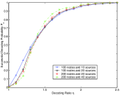
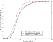
Figure 3: Decoding performance of the RCDS-I algorithm: (a) small number of nodes and sources; (b) large number of nodes and sources

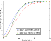
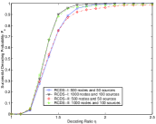
Figure 4: Decoding performance comparison of the RCDS-I and RCDS-II algorithms: (a) small number of nodes and sources; (b) large number of nodes and sources

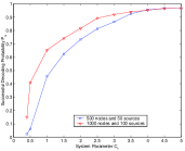
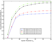
Figure 5: Impact of system parameters: (a) decoding performance of RCDS-I algorithm with different $C_{1}$, (b) decoding performance of RCDS-I algorithm with different $C_{2}$.

Our simulation results are shown in Figures. 3,  4 and 5. Fig. 3 shows the decoding performance of RCDS-I algorithm with different number of nodes and sources. The network is deployed in $\mathcal{A}=[5,5]^{2}$, and the system parameter $C_{1}$ is set as $C_{1}=5$. From the simulation results we can see that when the decoding ratio is above 2, the successful decoding probability is about $95\%$. Another observation is that when the total number of nodes increases but the ratio between $k$ and $n$ and the decoding ratio $\eta$ are kept as constants, the successful decoding probability $P_{s}$ increase when $\eta\geq 1.4$ and decreases when $\eta<1.4$. That is because the more nodes we have, the more likely each node has the desired degree distribution. Fig. 4 compares the decoding performance of RCDS-II and RCDS-I algorithms. To guarantee each node obtain accurate estimations of $n$ and $k$, we set $C_{2}=50$. It can be seen that the decoding performance of the RCDS-II algorithm is a little bit worse than the RCDS-I algorithm when decoding ratio $\eta$ is small, and almost the same when $\eta$ is large. To investigate how the system parameter $C_{1}$ and $C_{2}$ affects the decoding performance of the RCDS-I and RCDS-II algorithms, we fix the decoding ratio $\eta$ and vary $C_{1}$ and $C_{2}$. The simulation results are shown in Fig. 5. It can be seen that when $C_{1}\geq 4$, $P_{s}$ keeps almost like a constant, which indicates that after $4n\log n$ steps, almost all source packet visit each node at least once. We can also see that when $C_{2}$ is chosen to be small, the performance of the RCDS-II algorithm is very poor. This is due to the inaccurate estimations of $k$ and $n$ of each node. When $C_{2}$ is large, for example, when $C_{2}\geq 40$, the performance is almost the same.

V Conclusion

In this paper, we studied Raptor codes based distributed storage algorithms for large-scale wireless sensor networks. We proposed two new decentralized algorithms RCDS-I and RCDS-II that distribute information sensed by $k$ source nodes to $n$ nodes for storage based on Raptor codes. In RCDS-I, each node has limited global information; while in RCDS-II, no global information is required. We computed the computational encoding and decoding complexity, and transmission costs of these algorithms. We also evaluated their performance by simulation.

References

- [1] S. A. Aly, Z. Kong, and E. Soljanin. Fountain codes based distributed storage algorithms for large-scale wireless sensor networks. IEEE/ACM International Conference on Information Processing in Sensor Networks (IPSN), pages 171–182, Sa. Louis, MO, April 21-24, 2008.
- [2] S. A. Aly, Z. Kong, and E. Soljanin. Fountain codes based distributed storage algorithms. US patent, Status: pending, October, 2007.
- [3] Avin C. and Ercal G. On the cover time of random geometric graphs. In Proc. 32nd International Colloquium of Automata, Languages and Programming, ICALP’05, Lisboa, Portugal, July, 2005.
- [4] A. G. Dimakis, V. Prabhakaran, and K. Ramchandran. Ubiquitous access to distributed data in large-scale sensor networks through decentralized erasure codes. In Proc. 4th IEEE Symposium on Information Processing in Sensor Networks (IPSN), Los Angeles, CA, USA, April, 2005.
- [5] A. Kamra, J. Feldman, V. Misra, and D. Rubenstein. Growth codes: Maximizing sensor network data persistence. In Proc. of ACM SIGCOMM 2006, Pisa, Italy, September, 2006.
- [6] Y. Lin, b. Li, and B. Liang. Differentiated data persistence with priority random linear code. In Proc. of 27th International Conference on Distributed Computing Systems (ICDCS’07), Toronto, Canada, June, 2007.
- [7] Y. Lin, B. Liang, and B. Li. Data persistence in large-scale sensor networks with decentralized fountain codes. In Proc. of IEEE INFOCOM 2007, Anchorage, AL, May, 2007.
- [8] R. Motwani and P. Raghavan. Randomized Algorithms. Cambridge University Press, 1995.
- [9] S. Ross. Stochastic Processes. Wiley, New York, second edition, 1995.
- [10] A. Shokrollahi. Raptor codes. IEEE Transactions on Information Theory, 52:2551–2567, 2006.
- [11] A. Shokrollahi. Raptor codes. In Proc. of IEEE ISIT 2004, Chicago, IL, USA, June 2004.