A Multiscale Model of Partial Melts 2: Numerical Results

Abstract

In a companion paper, equations for partially molten media were derived using two-scale homogenization theory. This approach begins with a grain scale description and then coarsens it through multiple scale expansions into a macroscopic model. One advantage of homogenization is that effective material properties, such as permeability and the shear and bulk viscosity of the two-phase medium, are characterized by cell problems, boundary value problems posed on a representative microstructural cell. The solutions of these problems can be averaged to obtain macroscopic parameters that are consistent with a given microstructure. This is particularly important for estimating the “compaction length” which depends on the product of permeability and bulk viscosity and is the intrinsic length scale for viscously deformable two-phase flow.

In this paper, we numerically solve ensembles of cell problems for several geometries. We begin with simple intersecting tubes as this is a one parameter family of problems with well known results for permeability. Using this data, we estimate relationships between the porosity and all of the effective parameters with curve fitting. For this problem, permeability scales as $\phi^{n}$, $n\sim 2-3$, as expected and the bulk viscosity scales as $\phi^{-m}$, $m\sim 1$, which has been speculated, but never shown directly for deformable porous media. The second set of cell problems add spherical inclusions at the tube intersections. These show that the permeability is controlled by the smallest pore throats and not by the total porosity, as expected. The bulk viscosity remains inversely proportional to the porosity, and we conjecture that this quantity is insensitive to the specific microstructure. The computational machinery developed can be applied to more general geometries, such as texturally equilibrated pore shapes. However, we suspect that the qualitative behavior of our simplified models persists in these more realistic structures. In particular, our hybrid numerical–analytical model predicts that for purely mechanical coupling at the microscale, all homogenized models will have a compaction length that vanishes as porosity goes to zero. This has implications for computational models, and it suggests that these models might not resist complete compaction.

Gindraft=false SIMPSON ET AL. A MULTISCALE MODEL OF PARTIAL MELTS G. Simpson, Department of Mathematics, University of Toronto, Toronto, ON M5S 2E4, Canada. (simpson@math.toronto.edu) M. Spiegelman, Department of Applied Physics and Applied Mathematics, Columbia University, New York, NY 10027, USA. Lamont-Doherty Earth Observatory, Palisades, NY 10964, USA. (mspieg@ldeo.columbia.edu) M. I. Weinstein, Department of Applied Physics and Applied Mathematics, Columbia University, 200 Mudd, New York, NY 10027, USA. (miw2103@columbia.edu)

1 Introduction

Partially molten regions in the Earth’s asthenosphere (e.g. beneath mid-ocean ridges or subduction zones) are usually modeled as a viscously deformable permeable media. Such models are typically composed of macroscopic equations for the conservation of mass, momentum and energy of each phase. In our companion paper, [Simpson et al.(2008a)Simpson, Spiegelman, and Weinstein], we derived several systems of governing equations for partially molten systems using homogenization. Briefly, we began with a grain scale description of two interpenetrating fluids, each satisfying the Stokes equations, coupled by their common interface. Several different macroscopic models could then be coarsened from this microscopic description, depending on our assumptions on the velocities, viscosities, and grain scale geometry.

An important feature of this approach is that macroscopic properties such as permeability, shear viscosity, and bulk viscosity naturally appear in the macroscopic equations, even if they are not defined at the grain scale. In particular, permeability and bulk viscosity are properties of the two-phase aggregate, not the volume averages of small scale variations. In contrast, previous work on the magma problem, including [McKenzie(1984), Bercovici and Ricard(2003), Bercovici and Ricard(2005), Bercovici(2007), Hier-Majumder et al.(2006)Hier-Majumder, Ricard, and Bercovici, Ricard(2007)], began with models much larger than the grain scale. There, the viscosities, permeability, and other closures were assumed and justified from other results. In contrast, homogenization derives these properties self-consistently.

While homogenization techniques appropriately inserts the constitutive relationships into the macroscopic equations, connecting them to the microstructure requires the solution of specific “cell problems.” For the physical system derived in [Simpson et al.(2008a)Simpson, Spiegelman, and Weinstein], there are actually a series of ten Stokes problems for both fluid and solid posed on the micro-scale (which can be reduced to four for micro-structures with sufficient symmetry).

In this paper, we numerically explore the cell problems to extract parameterizations of the various effective parameters in terms of porosity, a simple measurement of the microstructure. A feature of this work is to derive constitutive relationships for the bulk viscosity as a function of porosity, which is essential for describing compactible permeable media. In particular, we show that for a range of simple pore structure the effective bulk viscosity is related to the porosity as.

$$\zeta_{\textrm{eff.}}\propto\phi^{-1}$$

Our results and some additional theory suggest that this scaling is insensitive to the specific pore geometry.

Since permeability and bulk-viscosity can both be consistently related to the same microstructure, these calculations also allow us to study the “compaction length” [McKenzie(1984)]. At sufficiently low melt concentrations, it is approximately

$$\delta_{\mathrm{comp.}}\propto\sqrt{k_{\textrm{eff.}}\zeta_{\textrm{eff.}}}$$

which depends on the product of the derived permeability $k_{\textrm{eff.}}$ and bulk viscosity $\zeta_{\textrm{eff.}}$, both of which depend on the porosity. The compaction length is the intrinsic length scale in magma dynamics. This work suggests that under solely mechanical deformation,

$$\lim_{\phi\to 0}\delta_{\mathrm{comp.}}(\phi)=0,$$

implying that no mechanical mechanism prevents a region from compacting to zero porosity. This result also places strong resolution constraints on computational models of magma migration which may require a regularization for small porosities.

An outline of this work is as follows. In Section 2, we review several models of partially molten rock and highlight the constitutive relations. In Section 3, we demonstrate the process of assuming a cell geometry to extract computational closures for the macroscopic system. We revisit these closures in Section 4 for more general geometries to assess their robustness. Finally, in Section 5, we combine our numerics with the equations and examine the implications.

2 Review of Equations and Constitutive Relations

2.1 Macroscopic Equations

In [Simpson et al.(2008a)Simpson, Spiegelman, and Weinstein], we showcased three models for momentum conservation in a partially molten medium. They were distinguished by the assumed scalings for the relative velocities and viscosities between the fluid and solid phases, along with the connectivity of the pore network. One of them, dubbed Biphasic-I, was given by the equations:

$$\begin{split}0&=\overline{\rho}\mathbf{g}-\nabla P+\nabla\left[\left(\zeta_{\textrm{eff.}}-\frac{2}{3}\mu_{s}(1-\phi)\right)\nabla\cdot\mathbf{V}^{s}\right]\\ &\quad+\nabla\cdot\left[2{(1-\phi)\mu_{s}}e(\mathbf{V}^{s})\right]+\nabla\cdot\left[2\eta_{\textrm{eff.}}^{lm}e_{lm}(\mathbf{V}^{s})\right]\end{split}$$ (1a)

$$\phi(\mathbf{V}^{f}-\mathbf{V}^{s})=-\frac{k_{\textrm{eff.}}}{\mu_{f}}\left(\nabla P-\mathbf{g}^{f}\right)$$ (1b)

$$\nabla\cdot\left[\phi\mathbf{V}^{f}+(1-\phi)\mathbf{V}^{s}\right]=0$$ (1c)

Notation for his model may be found in Table 1. In particular, $k_{\textrm{eff.}}$ and $\zeta_{\textrm{eff.}}$ are the emergent permeability and bulk viscosity. $\eta_{\textrm{eff.}}$ is an auxiliary, tensorial, shear viscosity capturing grain scale anisotropy. All are related to the aforementioned cell problems. We highlight this case because (1a – 1c) is nearly identical to the models of McKenzie, Bercovici, Ricard, and others in the absence of melting and surface physics.

Table 1: Notation for macroscopic equations derived by homogenization.

Symbol	Meaning
$\delta_{\mathrm{comp.}}$	Compaction length
$e(\mathbf{v})$	Strain rate tensor, $e(\mathbf{v})=\frac{1}{2}(\nabla\mathbf{v}+(\nabla\mathbf{v})^{T})$
$\eta_{\textrm{eff.}}$	Supplementary anisotropic viscosity derived by homogenization
$\phi$	Porosity
$K$	Permeability tensor of the matrix derived by homogenization
$k_{\textrm{eff.}}$	Isotropic permeability of the matrix derived by homogenization
$\mu_{f}$	Shear viscosity of the melt
$\mu_{s}$	Shear viscosity of the matrix
$P$	Macroscopic (fluid) pressure derived by homogenization
$\rho_{f}$	Melt density
$\rho_{s}$	Matrix density
$\overline{\rho}$	Mean density, $\overline{\rho}=\rho_{f}\phi+(1-\phi)\rho_{s}$
$\mathbf{V}^{f}$	Macroscopic fluid velocity derived by homogenization
$\mathbf{V}^{s}$	Macroscopic solid velocity derived by homogenization
$\zeta_{\textrm{eff.}}$	Bulk viscosity of the matrix derived by homogenization

2.2 Constitutive Relations

The constitutive relations for the permeability and viscosity are fundamental to the dynamics of these models. Indeed, they are the source of much nonlinearity and it is useful to review some proposed closures. Notation for this appears in Table 2.

Table 2: Notation for constitutive relations in other models.

Symbol	Meaning
$\phi_{\ast}$	Critical porosity for activation of $\mu_{s+f}$ viscosity
$\kappa$	Permeability of the matrix
$\mu_{s+f}$	Shear viscosity of the matrix in the presence of melt
$\zeta_{s}$	Bulk viscosity of the matrix

At low porosity, it is common to relate permeability, $\kappa$, to porosity by a power law, $\kappa\propto\phi^{n}$. Estimates of $n$ vary, $n\sim 2-5$, [Scheidegger(1974), Bear(1988), Dullien(1992), Turcotte and Schubert(2002), McKenzie(1984), Doyen(1988), Cheadle(1989), Martys et al.(1994)Martys, Torquato, and Bentz, Faul et al.(1994)Faul, Toomey, and Waff, Faul(1997), Faul(2000), Koponen et al.(1997)Koponen, Kataja, and Timonen, Wark and Watson(1998), Wark et al.(2003)Wark, Williams, Watson, and Price, Cheadle et al.(2004)Cheadle, Elliott, and McKenzie]. For partially molten rocks, the exponent is better constrained by both analysis and experiment to $n\sim 2-3$.

For the matrix shear viscosity, [Hirth and Kohlstedt(1995a), Hirth and Kohlstedt(1995b), Kohlstedt et al.(2000)Kohlstedt, Bai, Wang, and Mei, Kelemen et al.(1997)Kelemen, Hirth, Shimizu, Spiegelman, and Dick, Kohlstedt(2007)] experimentally observed a melt weakening effect, which they fit to the curve:

$$\mu_{s+f}=\mu_{s}\exp\left(-\phi/\phi_{\ast}\right),\quad\phi_{\ast}=O(10^{-2})$$ (2)

$\mu_{s+f}$ is the shear viscosity of the solid matrix in the presence of melt; $\mu_{s}$ is the shear viscosity a melt-free matrix. In [Bercovici et al.(2001)Bercovici, Ricard, and Schubert, Bercovici and Ricard(2003)] and related works, the viscosity is weighted by $(1-\phi)$, which is also present in (1a). Reiterating, $\mu_{s+f}$ is a fitting of experimental data. Regardless, the shear viscosity is taken to be isotropic, and porosity weakening in other models.

Lastly, the bulk viscosity, $\zeta_{s}$, is often taken as $\zeta_{s}\propto\phi^{-m}$, $m\sim 0-1$, though $m$ is usually either zero or one. $m=0$ has often been used because the variation of bulk viscosity with porosity is poorly constrained by observations. [Scott and Stevenson(1984)] and others invoked the bore hole studies of ice by [Nye(1953)] to justify $m=1$. In that work, Nye considered the dynamics of individual spherical and cylindrical voids in an infinite medium. [Taylor(1954), Prud’homme and Bird(1978)] computed $m=1$, in the limit of small porosity, using models of incompressible fluids mixed with gas bubbles. [Schmeling(2000)] also employed $\zeta_{s}\propto\phi^{-1}$, citing studies for the analogous question of the effective bulk modulus of a fluid filled poroelastic medium. Those results rely on the self-consistent approximation methodology, treated in [Torquato(2002)]. Models in [Bercovici et al.(2001)Bercovici, Ricard, and Schubert, Bercovici and Ricard(2003)] and related works possess a $\phi^{-1}$ term that functions as a bulk viscosity, though it has a very different origin. [McKenzie(1984)] suggested using a metallurgical model of spheres due to [Arzt et al.(1983)Arzt, Ashby, and Easterling] which considered a range of mechanisms for densification of powders under hot isostatic pressing. For viscous compaction mechanisms, the Arzt result recover a bulk viscosity proportional to $\phi^{-1}$ for Newtonian viscosities. However, for very small porosities, they suggest that surface diffusion effects become important and imply that $\zeta_{s}\propto\log(\phi^{-1})$. Finally, [Connolly and Podladchikov(1998)] invoke an assymetric bulk viscosity that is weaker during expansion than during compaction, which is motivated by the deformation of brittle crustal materials. However, it is unclear if this rheology is relevant to high-temperature/high-pressure creeping materials as are expected in the mantle. In general, it is expected that the bulk-viscosity should become unbounded as the porosity reduces to zero as the system then becomes incompressible.

2.3 Cell Problems

In homogenization, a medium with fine scale features is modeled by introducing two or more spatial scales. As discussed in [Simpson et al.(2008a)Simpson, Spiegelman, and Weinstein], the direct approach makes multiple scale expansions of the dependent variables, letting them depend on both the coarse and fine length scales.

The two characteristic lengths in our model are $L$, the macroscopic scale, and $\ell$, the grain scale. Their ratio,

$$\epsilon=\frac{\ell}{L}$$

is the parameter in which we perform the multiple scale expansions. In the process of performing the expansions and matching powers of $\epsilon$, we are mathematically constrained to solve a collection of auxiliary cell problems posed on the fine scale. Notation for this setup is provided in Table 3.

Table 3: Notation for cell problems.

Symbol	Meaning
$\epsilon$	Ratio of microscopic and macroscopic length scales, $\epsilon=\ell/L$
$e_{y}(\mathbf{v})$	Strain rate tensor, $e_{y}(\mathbf{v})=\frac{1}{2}(\nabla_{y}\mathbf{v}+(\nabla_{y}\mathbf{v})^{T})$
$\gamma$	Interface between melt and matrix within cell $Y$
$\ell$	Grain length scale
$L$	Macroscopic length scale
$\nabla_{y}$	Gradient taken with respect to the $\mathbf{y}$ argument
$\nabla_{y}\cdot$	Divergence taken with respect to the $\mathbf{y}$ argument
$\Omega$	Macroscopic region containing both melt and matrix
$\mathbf{y}$	Coordinate within the cell, $Y$
$Y$	The unit cell
$Y_{f}$	Portion of unit cell occupied by melt
$Y_{s}$	Portion of unit cell occupied by matrix
$\zeta$	Pressure of the cell problem for a unit forcing on the divergence equation

It is analytically advantageous to approximate the mixture as a periodic medium; such a configuration appears in Figure 1. $\Omega$, the macroscopic region containing both matrix and melt is periodically tiled with scaled copies of the cell, scaled to unity in Figure 2. The cell problems are posed within $Y_{s}$, the matrix portion of the cell, and $Y_{f}$, the melt portion for the cell. $Y_{s}$ and $Y_{f}$ meet on interface $\gamma$.

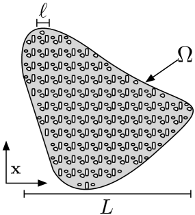
Figure 1: The macroscopic domain $\Omega$. The gray body is occupied by the matrix and the white inclusions are the melt.

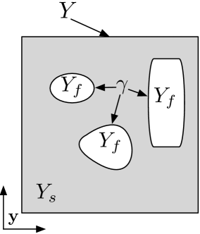
Figure 2: The cell domain, $Y$, divided into fluid and solid regions, $Y_{f}$ and $Y_{s}$. The two phases meet on interface $\gamma$.

Generically, the cell problems take the form:

$$\nabla_{y}\cdot\left(-pI+2e_{y}(\mathbf{v})\right) =\mathbf{f}\quad\text{in $Y_{f}$ or $Y_{s}$}$$ (3a)

$$\nabla_{y}\cdot\mathbf{v} =g\quad\text{in $Y_{f}$ or $Y_{s}$}$$ (3b)

$$\left(-pI+2e_{y}(\mathbf{v})\right)\cdot\mathbf{n} =\tau\cdot\mathbf{n}\quad\text{or}\quad\mathbf{u}=\mathbf{U}\quad\text{on $\gamma$}$$ (3c)

which are generally, compressible Stokes flow problems for the microscopic solid and melt velocities and pressures $(\mathbf{v},p)$. Here, $\nabla_{y}$ is the gradient, $\nabla_{y}\cdot$ is the divergence, and $e_{y}$ the strain-rate operator defined on the fine length scale $y$. A more complete description is given in [Simpson et al.(2008a)Simpson, Spiegelman, and Weinstein]. $\mathbf{f}$, $g$, $\tau$, and $\mathbf{U}$ are prescribed forcing functions on the relevant portion of $Y$, either $Y_{s}$ or $Y_{f}$. The solution, $(\mathbf{v},p)$, is periodic on the portion of the boundary not intersecting the interface $\gamma$. The cell problems may be interpreted as the fine scale response to an applied stress on a unit cell of either the melt or the matrix. The material parameters – $k_{\textrm{eff.}}$, $\zeta_{\textrm{eff.}}$, and $\eta_{\textrm{eff.}}$ – are then defined as the cell average of an appropriate manipulation of these pressures and velocities defined at the pore scale. In particular, an average of the solid pressure in one problem determines the bulk viscosity and certain averages of melt velocities in another problem determine the permeability. Again, we emphasize that the material parameters are not volume averages of the same parameters at the fine scale.

Table 4: Notation for cell problems, continued.

Symbol	Meaning
$\bar{\chi}^{lm}$	Velocity of the cell problem for a unit shear stress forcing on the solid in the $lm$ component of the stress tensor
$\mathbf{e}_{i}$	Unit vector in the i–th coordinate, $\mathbf{e}_{1}^{T}=(1,0,0)$
$\phi_{\textrm{eff.}}$	Effective porosity, portion of the porosity in which there is appreciable flow. $\phi_{\textrm{eff.}}\leq\phi$.
$\mathbf{k}^{i}$	Velocity of the cell problem for a unit forcing on the fluid in the $\mathbf{e}_{i}$ direction
$\mathbf{k}_{1}^{1}$	First component of the velocity from the cell problem with unit forcing on the fluid in the $\mathbf{e}_{1}$ direction
$\bar{\xi}$	Velocity of the cell problem for a unit forcing on the divergence equation
$\langle\cdot\rangle_{f}$	Volume average of a quantity over the melt portion of a cell, $\langle\cdot\rangle_{f}=\int_{Y_{f}}\cdot d\mathbf{y}$
$\langle\cdot\rangle_{s}$	Volume average of a quantity over the matrix portion of a cell, $\langle\cdot\rangle_{s}=\int_{Y_{s}}\cdot d\mathbf{y}$
$\pi^{lm}$	Pressure of the cell problem for a unit shear stress forcing on the solid in the $lm$ component of the the stress tensor
$q^{i}$	Pressure of the cell problem for a unit forcing on the fluid in the $\mathbf{e}_{i}$ direction
$\zeta$	Pressure of the cell problem for a unit forcing on the divergence equation

3 Effective Parameters: Intersecting Tube Geometry

To connect the effective material properties – $\eta_{\textrm{eff.}}$, $k_{\textrm{eff.}}$, and $\zeta_{\textrm{eff.}}$ – with the porosity, we must solve the cell problems and extract a parameterization. Unfortunately, the solution of the Stokes equations in a generic three dimensional domain lacks an analytic representation. Thus we compute the solutions to the cell problems numerically and fit the results to appropriate parameterized constitutive models. Notation for this section is summarized in Table 4.

As a first example of numerically closing the constitutive relations in a homogenization based model, we study the cell domain of triply intersecting cylinders, pictured in Figure 3. The fluid occupies the cylinders while the solid is the complementary portion of the cube. While this geometry is an oversimplification of real pore-geometries, it serves as proof of concept of the unified, self-consistent homogenization algorithm. Additionally, it serves as a numerical check since the permeability for this problem is expected to scale as $\phi^{2}$. In Section 4 we examine a generalization of this geometry.

In what follows, we emphasize that the information given by the parameterizations should be read with a certain skepticism. The order of magnitude and signs of the coefficients and exponents are of greater utility than the particular numbers.

We remark here that for the intersecting tube geometry, the tube radius scaled to the cell-size, $b$, can be explicitly related to the porosity:

$$\phi=3\pi b^{2}-8\sqrt{2}b^{3}$$ (4)

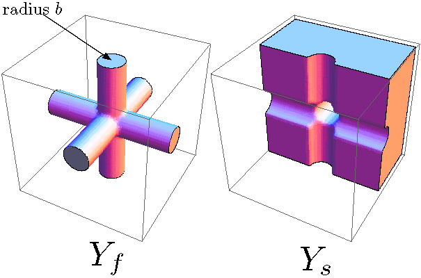
Figure 3: A cell geometry composed of triply intersecting cylinders of equal radius.

We solve our problems using finite elements on unstructured meshes using the open source libraries from the FEniCS and PETSc projects [[, e.g.]]DupHof2003,KirLog2007,Log2007,petsc-user-ref,petsc-web-page, with meshes generated using CUBIT [Sandia Corporation(2008)]. Details of this method and numerical benchmarks are given in Appendix B.

3.1 Effective Permeability

The first cell problem we treat is for permeability. The equations are:

$$-\nabla_{y}q^{i}+\nabla_{y}^{2}\mathbf{k}^{i} =-\mathbf{e}_{i}\quad\text{in $Y_{f}$}$$ (5a)

$$\nabla_{y}\cdot\mathbf{k}^{i} =0\quad\text{in $Y_{f}$}$$ (5b)

$$\mathbf{k}^{i} =0\quad\text{on $\gamma$}$$ (5c)

where $\mathbf{k}^{i}$ is a three-dimensional velocity and $q^{i}$ is a scalar pressure, for each $i=1,2,3$. These are equations (64a – 64c) in [Simpson et al.(2008a)Simpson, Spiegelman, and Weinstein] and describe the motion of the melt through the porous matrix. In general, the permeability is the second order tensor:

$$\langle K\rangle_{f}=\begin{bmatrix}\int_{Y_{f}}{\mathbf{k}^{1}}d\mathbf{y}&\int_{Y_{f}}{\mathbf{k}^{2}}d\mathbf{y}&\int_{Y_{f}}{\mathbf{k}^{3}}d\mathbf{y}\end{bmatrix}$$

The symmetry properties of the domain simplify this to:

$$\langle K\rangle_{f}=\langle\mathbf{k}_{1}^{1}\rangle I,\quad\textrm{$\mathbf{k}_{1}^{1}$ is the first component of vector $\mathbf{k}^{1}$}$$

Thus, it is sufficient to compute the case $i=1$. Then $k_{\textrm{eff.}}$, the permeability of the matrix, in (1b) is

$$\boxed{k_{\textrm{eff.}}\equiv\langle\mathbf{k}_{1}^{1}\rangle_{f}}$$ (6)

Darcy’s Law and permeability have been studied by many techniques, including homogenization; we refer the reader to the references in Section 2.2. We study it here to understand how the permeability behaves in concert with the other constitutive relations as the microstructure varies. This also serves as a benchmark problem for our software; see Appendix B.

As noted, porosity and permeability are often related by a power law, $\kappa\propto\phi^{n}$, with $n\sim 2-5$. To motivate such a relation, we turn to a toy model, as presented in [Turcotte and Schubert(2002)]. The melt is assumed to be in Poiseuille flow through triply intersecting cylinders. Additionally, the cylinders have small radii; it is a low porosity model. The permeability of such a system is

$$\kappa_{\textrm{toy-I}}=\frac{\ell^{2}\phi^{2}}{72\pi}\approx 0.0044\ell^{2}\phi^{2}.$$ (7)

Other simple models are developed in [Scheidegger(1974), Bear(1988), Dullien(1992)].

We now fit our computed permeabilities, $\langle\mathbf{k}_{1}^{1}\rangle$, to porosity by such a relation. For the tube domains, the least squares fit is

$$\langle\mathbf{k}^{1}_{1}\rangle_{f}=\exp(-4.42\pm.105)\phi^{2.20\pm.0391}.$$ (8)

This curve and the data appear in Figure 4. The fit matches expectations of an $O(10^{-3}-10^{-2})$ prefactor and an exponent $\sim 2-3$. The error in (8) is the associated 95% confidence interval. We report these intervals in all regressions, though they rely on the specious assumption that error in our synthetic data is normally distributed.

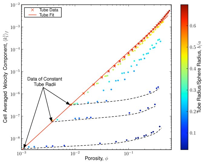
Figure 4: Numerically computed values of $\langle\mathbf{k}_{1}^{1}\rangle_{f}$, the effective permeability, plotted against porosity for both the tube geometry and the sphere+tube geometry. The scattered circles are data from sphere+tube geometries, colored by the ratio of tube radius to sphere radius. The tube geometry offers an upper bound for a given porosity.

3.2 Effective Bulk Viscosity

The effective bulk viscosity is related to the solution $(\bar{\xi},\zeta)$ of:

$$\nabla_{y}\cdot\left(-\zeta I+2e_{y}(\bar{\xi})\right) =0\quad\text{in $Y_{s}$}$$ (9a)

$$\nabla_{y}\cdot\bar{\xi} =1\quad\text{in $Y_{s}$}$$ (9b)

$$\left(-\zeta I+2e_{y}(\bar{\xi})\right)\cdot\mathbf{n} =0\quad\text{on $\gamma$}$$ (9c)

where $\bar{\xi}$ is a three-dimensional velocity and $\zeta$ is a scalar pressure. These are equations (B1a – B1c) in [Simpson et al.(2008a)Simpson, Spiegelman, and Weinstein] and are associated with the compaction of the matrix. The effective bulk viscosity is then defined as

$$\boxed{\zeta_{\textrm{eff.}}\equiv\mu_{s}\langle\zeta\rangle_{s}-\frac{2}{3}\mu_{s}(1-\phi)}$$ (10)

The dependence of the effective bulk viscosity of partially molten rock as a function of porosity is the most poorly constrained of the material properties. This is partly due to the difficulties in constructing an experiment that will measure it as a function of porosity independently of the shear viscosity [McKenzie(1984), Kelemen et al.(1997)Kelemen, Hirth, Shimizu, Spiegelman, and Dick, Stevenson and Scott(1991)]. As mentioned in Section 2.2, a bulk viscosity $\propto\phi^{-1}$ has often appeared in the literature.

Two toy models for the bulk viscosity of an incompressible fluid seeded with compressible gas bubbles were formulated by [Taylor(1954), Prud’homme and Bird(1978)]. They relate the bulk viscosity to the porosity as:

$$\zeta_{s} =\frac{4}{3}\frac{\mu_{s}}{\phi}$$ Taylor (11a)

$$\zeta_{s} =\frac{4}{3}\frac{\mu_{s}}{\phi}\left(1-\phi\right)$$ Prud’homme and Bird (11b)

Taylor’s expression, (11a), relied on a single inclusion model for a gas bubble in an infinite medium. (11b) is derived by considering a sphere of fluid with a gas filled spherical cavity, and seeking the bulk viscosity of a compressible fluid that will give rise to the same radial stress for specified boundary motion. The $1-\phi$ is due to Prud’homme and Bird restricting their model to a finite volume. This factor also appears in the proposed bulk viscosity of [Schmeling(2000)]. These expressions have motivated the use of $\zeta_{s}\propto\phi^{-1}$ in macroscopic models of partial melts, although they actually arise from a different problem of a compressible inclusion in an incompressible fluid, rather than the divergent flow of two interconnected incompressible fluids. Surprisingly, when we consider a simple toy problem to approximate the the full cell calculation, we find that the expressions are identical.

Appendix A provides details of this toy problem, which is related to equations (9a – 9c), and gives the solution

$$\langle\zeta\rangle_{s}=\frac{4}{3\phi}\left(1+\frac{\phi}{2}\right)\left(1-\phi\right),$$

from which we get

$$\zeta_{\textrm{eff.}}=\frac{4\mu_{s}}{3\phi}\left(1-\phi\right).$$

This motivates trying to numerically fit $\langle\zeta\rangle_{s}$ to $(1-\phi)^{p}/\phi^{q}$, expecting $p$ and $q$ to be close to unity. Indeed, the data, plotted in Figure 5, fits the curve

$$\langle\zeta\rangle_{s}=\exp(-0.131\pm 0.00514)\phi^{-1.02\pm 0.00132}(1-\phi)^{0.884\pm 0.00869}$$ (12)

which is quite similar to the scaling of the toy model.

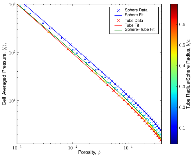
Figure 5: Numerically computed data for the dilation stress cell problem, (9a–9c), on the three geometries, along with the least square fits (12), (26a), and (26b)). The scattered circles are data from sphere+tube geometries, colored by the ratio of tube radius to sphere radius. The sphere+tube data is bounded between the the tube data and the sphere data.

3.3 Supplementary Anisotropic Viscosity

We now examine the cell problem related to the supplementary viscosity $\eta_{\textrm{eff.}}$, a fourth order tensor. The equations are:

$$\nabla_{y}\cdot\left(-\pi^{lm}I+2e_{y}(\bar{\chi}^{lm})\right) =0\quad\text{in $Y_{s}$}$$ (13a)

$$\nabla_{y}\cdot\bar{\chi}^{lm} =0\quad\text{in $Y_{s}$}$$ (13b)

$$\left(-\pi^{lm}\delta_{ij}+2e_{y,ij}(\bar{\chi}^{lm})\right)n_{j} =-\frac{1}{2}\left(\delta_{il}\delta_{jm}+\delta_{im}\delta_{jl}\right)n_{j}\quad\text{on $\gamma$}$$ (13c)

where $\bar{\chi}^{lm}$ is a three-dimensional velocity vector and $\pi^{lm}$ is a scalar pressure, for each pair $(l,m)$, $l=1,2,3$ and $m=1,2,3$. These are equations (B2a – B2c) from [Simpson et al.(2008a)Simpson, Spiegelman, and Weinstein] and are tied to tensorial surface stresses applied on the matrix. Using the solutions $(\bar{\chi}^{lm},\pi^{lm})$,

$$\boxed{\eta_{\textrm{eff.}}^{lm}\equiv\langle e_{y}(\bar{\chi}^{lm})\rangle_{s}}$$ (14)

Because of symmetry, we need only consider two problems: $(l,m)=(1,1)$ and $(l,m)=(1,2)$, corresponding to normal stress and shear stress in each direction.

Although we have no toy problem as motivation, $\phi^{p}(1-\phi)^{q}$ proved to be satisfactory. First, we study the problem $(l,m)=(1,1)$, a uniaxial stress problem. For the tubes, we fit

$$-\langle e_{1,1}(\bar{\chi}^{11})\rangle_{s}=\exp(-1.72\pm.0405)\phi^{.964\pm.0104}(1-\phi)^{1.23\pm.0685}$$ (15)

This vanishes as $\phi\to 0$ and as $\phi\to 1$ and it is nearly linear at small porosity. The curves and the data are plotted in Figure 6.

Figure 6: Numerically computed data for the normal stress cell problem on the three geometries, along with the least square fits (15), (27a), and (27b). The scattered circles are data from sphere+tube geometries, colored by the ratio of tube radius to sphere radius. At small porosity there is little variation amongst the simulated domains.

There is also the simple shear stress problem, $(l,m)=(1,2)$. For this, we fit

$$-\langle e_{12}(\bar{\chi}^{(12)})\rangle_{s}=\exp(-1.04\pm.0188)\phi^{1.06\pm.00485}(1-\phi)^{1.17\pm.0318}$$ (16)

Plots for this are given in Figure 7.

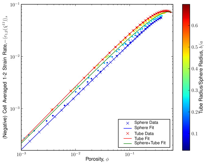
Figure 7: Numerically computed data for the shear stress cell problem on the three geometries, along with the least square fits (16), (28a), (28b). The scattered circles are data from sphere+tube geometries, colored by the ratio of tube radius to sphere radius. Sphere+Tube data points are constrained between the sphere data and the tube data. At all simulated porosities, there is less than an order of magnitude of variation.

We could now employ the simple computational closures (8), (12), (15), and (16), in (1a – 1c), to simulate and study the macroscopic problem.

4 Generalization of the Cell Domains

Regrettably, Earth materials are not as trivial as intersecting cylinders. Even an idealized olivine grain is a tetrakaidekahedron, pictured in Figures 8. As depicted, some fraction of the melt lies along the triple junctions and some is at the quadruple junctions. Other examples of idealized, texturally equilibrated arrangements appear in [von Bargen and Waff(1986)] and [Cheadle(1989), Cheadle et al.(2004)Cheadle, Elliott, and McKenzie]. These methods are also amenable to studying random media. One could compute relations based on ensembles of randomly generated cell domains, solving all relevant cell problems on the ensemble.

Figure 8: An idealized Olivine grain from Figure 1 of [Zhu and Hirth(2003)]. Melt channels are found at triple junctions, while melt pockets are found quadruple junctions.

Motivated by Figure 8, we explore a simple generalization of the tube geometry by adding a sphere of independent radius at the intersection, as in Figure 9. This retains the symmetry of the previous model, but adds a second parameter, allowing multiple geometries for the same porosity. The sphere captures some aspect of the pocket at the quadruple junctions. The sphere radius, $a$, and the tube radius, $b$, are related to the porosity by the equation:

$$\phi=\pi\left[-4a^{3}+4a^{2}\sqrt{a^{2}-b^{2}}+b^{2}\left(3-4\sqrt{a^{2}-b^{2}}\right)+\frac{4}{3}a^{3}\right]$$ (17)

We shall refer to it as the sphere+tube geometry.

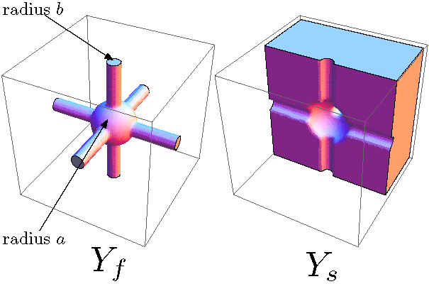
Figure 9: A cell geometry composed of triply intersecting cylinders of equal radius, with a sphere at the intersection.

We now repeat the computations of Section 3 on the sphere+tube geometry to assess the sensitivity of the effective parameters to cell geometry. We also perform computations on domains where the fluid occupies an isolated sphere at the center of a cube. Though this is disconnected, it provides useful information.

4.1 Permeability Revisited

Parameterizing the porosity-permeability relation for this generalization is quite challenging. In contrast to the tube geometry, the data points of the sphere+tube geometry, plotted in Figure 4, do not collapse onto a curve. There is some positive correlation between permeability and porosity, and for a given porosity, the permeability of the equivalent tube geometry is an upper bound.

To better understand the trend, we examine the computed flow fields in Figures 10 and 11. These plot the velocity magnitude on two fluid domains with the same tube size, but different sphere sizes. Most of the flow is within the tube. While there is some detrainment as it enters the sphere, the flow in the tube appears insensitive to the size of the sphere.

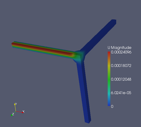
Figure 10: The magnitude of the velocity for a permeability cell problem. This corresponds to the sphere+tube domain with sphere radius $a=.06$ and tube radius $b=.03$.

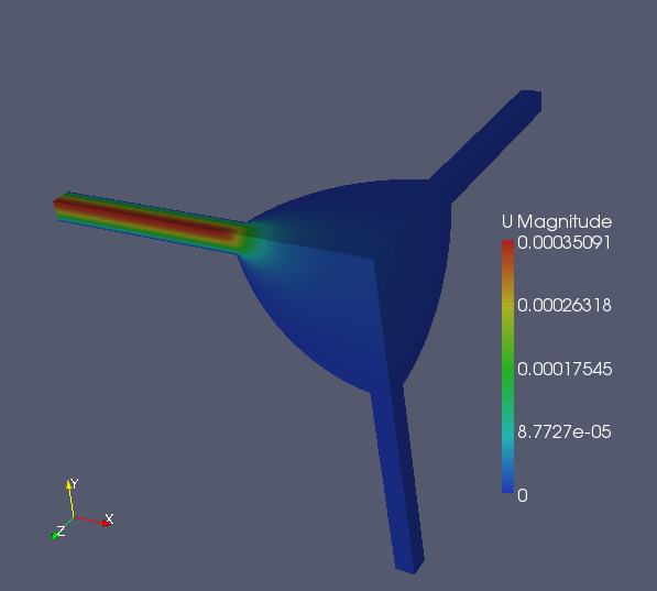
Figure 11: The magnitude of the velocity for a permeability cell problem. This corresponds to the sphere+tube domain with sphere radius $a=.20$ and tube radius $b=.03$.

This motivates fitting permeability against tube radius. Indeed, an alternative to (7), is

$$\kappa_{\textrm{toy-II}}=\frac{\delta^{4}}{128\ell^{2}}$$ (18)

The tube diameter $\delta$, is equivalent to $2b$, $b$ the the tube radius in the tube and sphere+tube geometries. Both data sets appear in Figure 12. This is a significant improvement over Figure 4. The least square fits are:

$$\langle\mathbf{k}_{1}^{1}\rangle_{f} =\exp(-0.592\pm.0354)b^{4.10\pm.0156},\quad\text{for tube geometry}$$ (19)

$$\langle\mathbf{k}_{1}^{1}\rangle_{f} =\exp(-0.628\pm.198)b^{3.93\pm.0684},\quad\text{for sphere+tube geometry}$$ (20)

These estimates with (18); taking $\delta=2b$ and scaling out $\ell$, this relationship is $k_{\textrm{toy-II}}=.125b^{4}$. The data is still positively correlated with sphere radius, altering it by as as much as an order of magnitude. The deviations are greatest when both $b\ll 1$ and $b\ll a$.

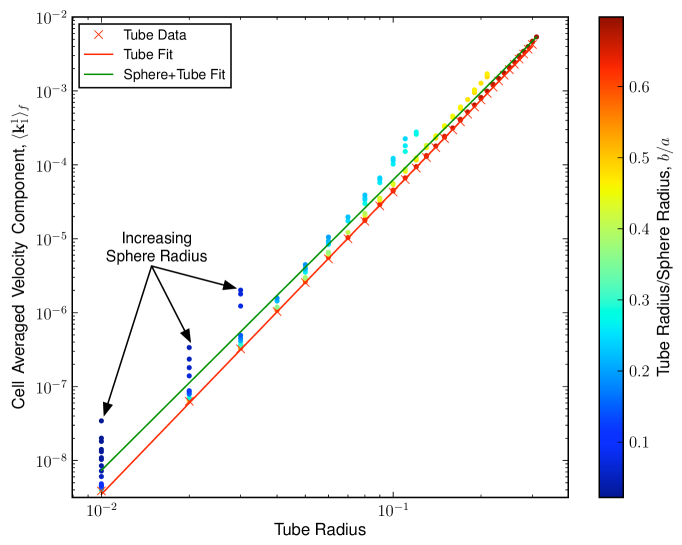
Figure 12: $\langle\mathbf{k}_{1}^{1}\rangle_{f}$, the effective permeability, plotted against tube radius for both the tube geometry and the sphere+tube geometry. The scattered circles are data from sphere+tube geometries, colored by the ratio of tube radius to sphere radius. The tube geometry offers a lower bound for a given porosity.

.

That the permeability is more strongly correlated with the tube radius than the overall geometry is not surprising. [Koponen et al.(1997)Koponen, Kataja, and Timonen] discuss the notion of effective porosity, the portion of the void space where there is significant flow. Denoting our effective porosity $\phi_{\textrm{eff.}}$, we seek a relation $k_{\textrm{eff.}}\propto\phi_{\textrm{eff.}}^{n}$.

Given the flow fields in Figures 10 and 11 and the success with the tube radius fittings, we posit that the effective porosity is the portion of the porosity within the tubes. A two-dimensional analog appears in Figure 13. Using (8), we define $\phi_{\textrm{eff.}}$ for the sphere+tube domains:

$$\phi_{\mathrm{eff.}}=3\pi b^{2}-8\sqrt{2}b^{3}$$ (21)

[Zhu and Hirth(2003)] made a similar approximation; from [von Bargen and Waff(1986)] they construed that the permeability was controlled by the minimal cross-sectional area of the pore network. A similar argument is made by [Cheadle(1989)]. In our domains, the minimal cross-sectional area is $\pi b^{2}$.

We fit

$$\langle\mathbf{k}_{1}^{1}\rangle_{f}=\exp(-4.44\pm.144)\phi_{{\textrm{eff.}}}^{2.06\pm.0374}\quad\text{for sphere+tube}.$$ (22)

This appears in Figure 14. Again, deviation is highest for very large spheres with very thin tubes. Unfortunately, $\phi_{\textrm{eff.}}$ does not satisfy a conservation law, making it a less than ideal macroscopic quantity to track, though it does satisfy the bound $\phi_{\textrm{eff.}}\leq\phi$.

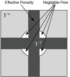
Figure 13: The dark portion is the postulated effective porosity for the sphere+tube domains.

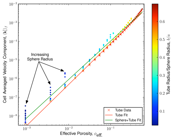
Figure 14: $\langle\mathbf{k}_{1}^{1}\rangle_{f}$, the permeability, plotted against the effective porosity for the sphere+tube geometry. The scattered circles are data from sphere+tube geometries, colored by the ratio of tube radius to sphere radius. The tube data plotted against porosity also appears.

There is still as much as an order of magnitude deviation at low porosity from relation (22). The unresolved part of the permeability for the $\phi_{\textrm{eff.}}$ fit is increasing in the sphere radius. This motivates trying to fit against both $\phi_{\textrm{eff.}}$ and another parameter. It is sufficient to fit permeability to $\phi_{\textrm{eff.}}$ and $\phi$, resulting in

$$\langle\mathbf{k}^{1}_{1}\rangle_{f}=\exp(-4.20\pm.0681)\phi_{\textrm{eff.}}^{1.88\pm.0229}\phi^{.351\pm.0300}\quad\text{for sphere+tube}.$$ (23)

This is plotted in Figure 15. Some deviation persists at low porosity, but it is less than an order of magnitude. Both the sphere+tube data points and the tube data points collapse onto this curve. (23) is also consistent with (8), the fit of porosity agaist permeability for the tube geometry. Taking $\phi_{\textrm{eff.}}=\phi$ for the tubes, (23) becomes

$$\langle\mathbf{k}^{1}_{1}\rangle_{f}=\exp(-4.20)\phi^{2.23}$$ (24)

This is similar to the most general permeability relationships, formulated in [Scheidegger(1974), Bear(1988)]:

$$\textrm{permeability}=\ell^{2}f_{1}(\textrm{pore shape})f_{2}(\phi)$$ (25)

By including both $\phi$ and $\phi_{\textrm{eff.}}$ in (23), we capture some aspect of the pore shape.

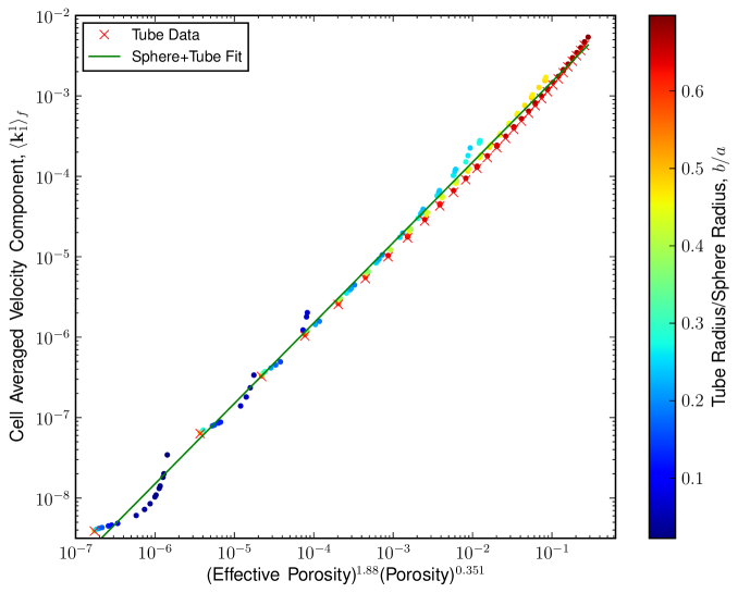
Figure 15: $\langle\mathbf{k}_{1}^{1}\rangle_{f}$, the permeability, plotted against the effective porosity and porosity, using (23). The scattered circles are data from sphere+tube geometries, colored by the ratio of tube radius to sphere radius. The tube data is also plotted, substituting $\phi$ for $\phi_{\textrm{eff.}}$ in (23).

4.2 Bulk and Supplementary Viscosities Revisited

In contrast to the permeability problem, the effective bulk viscosity and supplementary anisotropic viscosity are quite robust to the domain distortion. As before, we fit $\langle\zeta\rangle_{s}$ to $(1-\phi)^{p}/\phi^{q}$, expecting $p$ and $q$ to be close to unity. For the sphere+tube and the sphere geometry, the least squares fits are:

$$\langle\zeta\rangle_{s} =\exp(0.301\pm 0.0102)\phi^{-1.00\pm 0.00174}(1-\phi)^{0.718\pm 0.0337},\quad\text{for sphere geometry}$$ (26a)

$$\langle\zeta\rangle_{s} =\exp(0.124\pm 0.0975)\phi^{-0.985\pm 0.0252}(1-\phi)^{1.09\pm 0.186},\quad\text{for sphere+tube geometry}$$ (26b)

The data and these fits are plotted appear in Figure 5. The spherical geometry appears to be an upper bound on the bulk viscosity for a given porosity. We also remark that the prefactors vary by less than an order of magnitude amongst the different domains. This is a strong endorsement of an effective bulk viscosity$\propto\phi^{-1}$ not only for small porosity, but also for moderate porosities $\gtrsim 10\%$.

The supplementary anisotropic viscosity terms are also robust under this geometric perturbation. For the problem $(l,m)=(1,1)$, the two new geometries fit:

$$-\langle e_{1,1}(\bar{\chi}^{11})\rangle_{s} =\exp(-1.68\pm.0588)\phi^{.980\pm.0101}(1-\phi)^{3.56\pm.195},\quad\text{for sphere geometry}$$ (27a)

$$-\langle e_{1,1}(\bar{\chi}^{11})\rangle_{s} =\exp(-1.94\pm.139)\phi^{.912\pm.0359}(1-\phi)^{1.25\pm.265},\quad\text{for sphere+tube geometry}$$ (27b)

The curves and the data are also plotted in Figure 6. For $\phi\lesssim 10\%$, the spread amongst the three geometries is less than an order of magnitude.

Similar results are found in the $(l,m)=(1,2)$ problem. The two new additional domains are fit with:

$$-\langle e_{12}(\bar{\chi}^{(12)})\rangle_{s} =\exp(-1.67\pm.0222)\phi^{1.02\pm.000380}(1-\phi)^{0.400\pm.0737},\quad\text{for sphere geometry}$$ (28a)

$$-\langle e_{12}(\bar{\chi}^{(12)})\rangle_{s} =\exp(-1.32\pm.00883)\phi^{1.03\pm.00228}(1-\phi)^{0.871\pm.169},\quad\text{for sphere+tube geometry}$$ (28b)

The sphere+tube data is bounded between the sphere data and the tube data; the spread is less than an order of magnitude.

5 Discussion and Open Problems

We have successfully parameterized the macroscopic parameters on ensemble of domains for the simple pore geometries. These can now be consistently used with the macroscopic model given by equations (1a – 1c). We now review and discuss our computations, both independently of and together with the macroscopic equations.

5.1 Sensitivity to Geometry

As demonstrated by our computations in Sections 3 and 4, the effective parameters demonstrate a variety of sensitivities to the geometry. Permeability, for our cell geometries, can be bounded by porosity, $k_{\textrm{eff.}}\lesssim\phi^{n}$, where $n\sim 2$, as seen in Figure 4. But in general, it cannot be expressed as a function of a single parameter, such as porosity. However, if the shapes are constrained by textural equilibration, as in [Cheadle(1989)], there will be a single variable parameterization for each dihedral angle. Solving the cell problems on these shapes, and assessing their sensitivity to the dihedral angle, is an important open problem.

In contrast, the bulk viscosity appears to be rather insensitive to the geometry, scaling as $\zeta_{\textrm{eff.}}\propto\phi^{-1}(1-\phi)$. We see this from the variation, or lack thereof, between the data and fits for the isolated spheres and the triply intersecting cylinders, in Figure 5. Though these are entirely different geometric structures, there is less than an order of magnitude of variation in the computed $\zeta_{\textrm{eff.}}$. These too merit computation on the texturally equilibrated shapes. Randomly generated geometries may also be of interest.

Both components of the supplementary anisotropic shear viscosity appear to be insensitive to geometry, with less than an order of magnitude amongst the three geometries. However, because the problems are driven by surface stresses, it may be that a more anisotropic shape could alter these scalings. Studying them on randomly generated shapes may provide insight on the role of grain scale anisotropy.

5.2 Bulk Viscosity

Perhaps our most significant result is the self-consistent bulk viscosity, arising from a purely mechanical model of partially molten rock. A spatially varying bulk viscosity is quite important. Indeed, significant differences in dynamics were noted between the solutions of the [McKenzie(1984)] model and the model in [Ricard et al.(2001)Ricard, Bercovici, and Schubert]. The authors point to the use of a constant bulk viscosity in the McKenzie model as the source of the discrepancy.

Prior to [Ricard et al.(2001)Ricard, Bercovici, and Schubert], [Schmeling(2000)] remarked that the $\phi^{-1}$ dependence has an important impact on the compaction length. For $\phi=O(1\%)$, the bulk viscosity is two orders of magnitude greater than the shear viscosity. While many studies took $\zeta_{s}$ and $\mu_{s}$ to be the same order, this higher bulk viscosity leads to a compaction length an order of magnitude greater. [Ricard(2007)] made a similar observation on the impact of variable bulk viscosity on the compaction length.

Schmeling also commented that this variable bulk viscosity could induce melt focusing towards the axis in his plume simulations. This is an additional nonlinearity that may be important to geophysical problems. Many studies relying on the McKenzie model employed a constant bulk viscosity, including [Richter and McKenzie(1984), Spiegelman and McKenzie(1987), Spiegelman(1993a), Spiegelman(1993b), Spiegelman(1993c), Aharonov et al.(1997)Aharonov, Spiegelman, and Kelemen, Spiegelman(1996), Kelemen et al.(1997)Kelemen, Hirth, Shimizu, Spiegelman, and Dick, Spiegelman et al.(2001)Spiegelman, Kelemen, and Aharonov, Katz et al.(2004)Katz, Spiegelman, and Carbotte, Spiegelman et al.(2007)Spiegelman, Katz, and Simpson]. [Spiegelman and Kelemen(2003), Spiegelman(2003)] used a bulk viscosity, with $\zeta_{s}\propto\phi^{-m}$ with $m>n$, $n$ the exponent in the permeability relationship $\kappa\propto\phi^{n}$ to prevent the system from compacting to zero between the reactive channels. It would be interesting to revisit these problems with a $\phi^{-1}$ bulk viscosity.

5.3 Compaction Length

We now combine (1a – 1c), our leading order equations derived by multiple scale expansions, with our computed constitutive relations. For $\phi\ll 1$ our numerical estimates, (23), (26a–26b), (15–27b), (27a), and (16–28a) are approximately:

$$\zeta_{\textrm{eff.}} \approx\mu_{s}\zeta_{0}\phi^{-1}(1-\phi)$$

$$\eta_{\textrm{eff.}} \approx\mu_{s}\eta_{0}\phi(1-\phi)$$

$$k_{\textrm{eff.}} \approx k_{0}\ell^{2}\phi_{\textrm{eff.}}^{1.9}\phi^{.35}$$

$k_{0}$ is a $O(10^{-3}-10^{-2})$ constant, $\zeta_{0}$ is an $O(1)$ constant, and $\eta_{0}$ is a $O(10^{-1})$ constant fourth order tensor. Under these assumptions, the equations for the Biphasic-I model, (1a – 1c), simplify:

$$\begin{split}0&=\overline{\rho}\mathbf{g}-\nabla P+\nabla\left[\mu_{s}\zeta_{0}\phi^{-1}\nabla\cdot\mathbf{V}^{s}\right]\\ &\quad+\nabla\cdot\left[2(1-\phi){\mu_{s}}e(\mathbf{V}^{s})-\frac{2}{3}(1-\phi)\mu_{s}\nabla\cdot\mathbf{V}^{s}I\right]\\ &\quad+\nabla\cdot\left[2\mu_{s}\phi(1-\phi)\eta_{0}^{lm}e_{x,lm}(\mathbf{V}^{s})\right]\end{split}$$ (29)

$$\phi(\mathbf{V}^{f}-\mathbf{V}^{s})=-\frac{k_{0}\ell^{2}\phi_{\textrm{eff.}}^{1.9}\phi^{.35}}{\mu_{f}}\left(\nabla P-\mathbf{g}^{f}\right)$$ (30)

$$\nabla\cdot\left[\phi{\mathbf{V}^{f}}+(1-\phi)\mathbf{V}^{s}\right]=0$$ (31)

If we were to use these equations and numerically derived constitutive relations to solve a boundary value problem, the compaction length would again appear as an important length scale,

$$\begin{split}\delta_{\textrm{comp.}}&=\sqrt{\frac{\left[\zeta_{\textrm{eff.}}+\frac{4}{3}\mu_{s}(1-\phi)+2\left|\eta_{\textrm{eff.}}\right|\right]k_{\textrm{eff.}}}{\mu_{f}}}\\ &\approx\ell\sqrt{\frac{\mu_{s}(1-\phi)(\zeta_{0}\phi^{-1}+\frac{4}{3}+2\left|\eta_{0}\right|\phi)k_{0}\phi_{\textrm{eff.}}^{1.9}\phi^{.35}}{\mu_{f}}}\end{split}$$

If $\phi\ll 1$, then $\zeta_{0}\phi^{-1}\gg 4/3+2\left|\eta_{0}\right|\phi$ and $1-\phi\approx 1$,

$$\delta_{\textrm{comp.}}\approx\ell\sqrt{\zeta_{0}k_{0}\mu_{s}/\mu_{f}}\phi^{-.325}\phi_{\textrm{eff.}}^{.95}$$ (32)

Since $\phi_{\textrm{eff.}}\leq\phi$, we have an upper bound on the compaction length,

$$\boxed{\delta_{\textrm{comp.}}\lesssim\ell\sqrt{\zeta_{0}k_{0}\mu_{s}/\mu_{f}}\phi^{.6}}$$ (33)

Hence,

$$\lim_{\phi\to 0}\delta_{\textrm{comp.}}=0$$

We believe (33), which constrains the compaction length by the porosity raised to a small positive power, is relatively insensitive to the geometric configuration. This follows from our alleged robustness of our effective bulk viscosity, $\zeta_{\textrm{eff.}}\propto\phi^{-1}$, and the broad agreement in the porosity–permeability relationship, $\kappa\propto\phi^{n}$ with $n\geq 2$.

A compaction length that vanishes with porosity has interesting consequences. For example, this compaction length scaling does not rule out the possibility that a partially molten rock could expel all fluid by mechanical means. It also does not permit the infiltration of fluid into a dry region. Understanding how any of these systems of equations transition between a partially molten region and a dry region is an outstanding question. We also note that though our scaling relationship does not forbid compaction, it does not imply it either. There may be a dynamic response that prevents the matrix from mechanically compacting to zero. Such effects were mathematically proven to exist in a one-dimensional simplification of the model, without melting or freezing, in [Simpson et al.(2007)Simpson, Spiegelman, and Weinstein, Simpson and Weinstein(2008), Simpson et al.(2008c)Simpson, Weinstein, and Rosenau].

If, instead, we had concluded $\delta_{\textrm{comp.}}\propto\phi^{q}$, with $q<0$, then the compaction length would become unbounded as the melt vanished. Hence the region of deformation in the matrix needed to segregate additional fluid would also become infinite, precluding further segregation solely by mechanical processes.

Because we have parameterized the permeability with $\phi_{\textrm{eff.}}$, we can explicitly see the response of the compaction length as the melt network becomes disconnected. $\phi_{\textrm{eff.}}$ measures the volume fraction where melt flows. As the channels close up and the melt becomes trapped and $\phi_{\textrm{eff.}}\to 0$. Taking this limit in (32),

$$\lim_{\phi_{\textrm{eff.}}\to 0}\delta_{\textrm{comp.}}=0$$

The compaction length can vanish, even if the melt fraction remains bounded away from zero. A similar conclusion could be drawn for the compaction length of McKenzie,

$$\delta_{\textrm{M84}}=\sqrt{\frac{\kappa(1-\phi)(\zeta_{s}+\frac{4}{3}\mu_{s})}{\mu_{f}}}$$ (34)

Letting $\kappa=\kappa_{0}\phi^{n}$, if we interpret the loss of connectivity as $\kappa_{0}\to 0$, $\delta_{\textrm{M84}}$ vanishes with nonzero porosity.

5.4 Other Physics

There are several results that were not realized by our model, and these merit discussion. We did not recover the $\zeta_{s}\propto\log(\phi^{-1})$ result of [Arzt et al.(1983)Arzt, Ashby, and Easterling]. This arises in the limit of sufficiently low porosity that the primary transport mechanism is by grain boundary diffusion. Since we did not include any surface physics in our fine scale model, we should not have expected to upscale their effects. If good grain scale descriptions of these processes could be formulated, it might be possible to coarsen them via homogenization, perhaps recovering this macroscopic relation. However, as $\log(\phi^{-1})$ becomes unbounded more slowly than $\phi^{-1}$, this result does not change the basic argument about the compaction length vanishing with zero porosity.

Another relationship not captured by either our work is the experimental fit for matrix shear viscosity in the presence of melt from [Hirth and Kohlstedt(1995a), Hirth and Kohlstedt(1995b), Kelemen et al.(1997)Kelemen, Hirth, Shimizu, Spiegelman, and Dick, Kohlstedt et al.(2000)Kohlstedt, Bai, Wang, and Mei, Kohlstedt(2007)],

$$\mu_{s+f}\propto\exp\left(-\phi/\phi_{\ast}\right)$$

Our model possesses a porosity weakening mechanism; all of the viscosity terms are $\propto 1-\phi$. However, the anisotropic part, $\eta_{\textrm{eff.}}$, is not sign definite and is small compared to the isotropic component. Furthermore, there does not appear to be an exponential relation. [Hirth and Kohlstedt(1995a)] hypothesized that the presence of melt enhances grain boundary diffusion, providing a fast path for deformation through the melt. As with the $\log(\phi^{-1})$ bulk viscosity, this is a surface physics phenomenon not captured by our Stokes models.

5.5 Open Problems

As discussed, two important open problems are the computation of the cell problems on more realistic and general cell domains and the inclusion of surface physics into the model. The former problem is rather straightforward, requiring good computational tools for generating the domains and solving the Stokes equations on them. The latter problem is more challenging, requiring fine scale equations for these processes.

The models could also be augmented by giving the matrix a nonlinear rheology, leading to nonlinear cell problems. Though these could be solved and studied numerically, this is much more difficult as the different forcing components no longer decouple. Rather than being able to split the matrix cell problems into a bulk viscosity problem, and two surface stress problems, they would have to be done simultaneously. However, the derived parameterizations for the effective viscosities would be important to magma migration. A nonlinear matrix rheology is expected at large strain rates and was needed to computationally model physical experiments for shear bands in [Katz et al.(2006)Katz, Spiegelman, and Holtzman].

Another important physical rheology is viscoelasticity. [Connolly and Podladchikov(1998), Vasilyev et al.(1998)Vasilyev, Podladchikov, and Yuen] extended the earlier, purely viscous, models to include elastic effects. This is an important regime since it permits both short and long time scales, as is found at the asthenosphere-lithosphere boundary.

Appendix A Spherical Model

Here we develop a toy model for equations (9a – 9c),

$$\nabla_{y}\cdot\left(-\zeta I+2e_{y}(\bar{\xi})\right) =0\quad\text{in $Y_{s}$}$$

$$\nabla_{y}\cdot\bar{\xi} =1\quad\text{in $Y_{s}$}$$

$$\left(-\zeta I+2e_{y}(\bar{\xi})\right)\cdot\mathbf{n} =0\quad\text{on $\gamma$}$$

whose solution yields the effective bulk viscosity,

$${\zeta_{\textrm{eff.}}=\mu_{s}\langle\zeta\rangle_{s}-\frac{2}{3}\mu_{s}(1-\phi)}$$

Consider a fluid domain, $Y_{f}$, occupying a small isolated sphere at the center of the unit cube; $Y_{s}$ is the complementary region. Smoothing out the exterior boundary of $Y_{s}$ deforms it into a sphere. We solve the dilation stress problem on this domain. To avoid confusion, let

$${Y_{s}}^{\textrm{sphere}} =\left\{\mathbf{y}\in\mathbb{R}^{3}\mid a\leq\left|\mathbf{y}\right|\leq 1\right\}$$ (35)

$${Y_{s}}^{\textrm{cube}} =\left\{\mathbf{y}\in\left[-\frac{1}{2},\frac{1}{2}\right]^{3}\mid\left|\mathbf{y}\right|\geq a\right\}$$ (36)

Our toy problem is posed on ${Y_{s}}^{\textrm{sphere}}$.

Although periodicity is no longer a meaningful boundary condition, it can be shown that the normal velocity on the periodic part of $\partial Y_{s}$ vanishes. We set the normal velocity to zero on the exterior boundary of ${Y_{s}}^{\textrm{sphere}}$. On the interior shell, the stress free condition remains. The equations are:

$$\nabla\cdot\left(-\zeta I+2e(\bar{\xi})\right) =0\quad\text{in ${Y_{s}}^{\textrm{sphere}}$}$$ (37a)

$$\nabla\cdot\bar{\xi} =1\quad\text{in ${Y_{s}}^{\textrm{sphere}}$}$$ (37b)

$$\left(-\zeta I+2e(\bar{\xi})\right)\cdot\mathbf{n} =0\quad\text{at $r=a$}$$ (37c)

$$\bar{\xi}\cdot\mathbf{n} =0\quad\text{at $r=1$}$$ (37d)

$a<1$ is the radius of the interior sphere. Decomposing the velocity into incompressible, $\mathbf{v}^{\mathrm{inc.}}$, and compressible, ${\nabla\Pi}$, components, the compressible part solves:

$$\nabla^{2}\Pi=1$$ (38)

Let the boundary conditions on the potential be:

$$\Pi|_{r=a}=0,\quad\nabla\Pi|_{r=1}=0$$ (39)

Since the problem is spherically symmetric, its solution is

$$\Pi=\frac{1}{6}(r^{2}-a^{2})+\frac{1}{3}(r^{-1}-a^{-1})$$ (40)

The incompressible velocity must be divergence free. Again, by spherical symmetry,

$$\nabla\cdot\mathbf{v}^{\mathrm{inc.}}=\frac{1}{r^{2}}\partial_{r}\left(r^{2}v_{r}^{\mathrm{inc.}}\right)=0\Rightarrow v_{r}^{\mathrm{inc.}}=C/r^{2}$$

To satisfy the boundary condition at $r=1$, $\mathbf{v}^{\mathrm{inc.}}\cdot\mathbf{n}=v_{r}^{\mathrm{inc.}}=0$. Therefore, $C=0$ and $\mathbf{v}^{\mathrm{inc.}}=0$. The pressure then solves $\partial_{r}\zeta=0$, so it is constant,

$$\zeta(r)=\zeta(a)\quad\text{for $r\in(a,1)$}$$

Applying boundary condition (37c),

$$\zeta=2e_{rr}(\bar{\xi})|_{r=a}=2\partial_{r}^{2}\Pi|_{r=a}=\frac{1}{3}\left(2+\frac{4}{a^{3}}\right)$$

In this geometry, $\phi=a^{3}$, and the cell averaged pressure is

$$\langle\zeta\rangle_{s}=\frac{4}{3\phi}\left(1+\frac{\phi}{2}\right)\left(1-\phi\right)$$ (41)

Therefore,

$$\zeta_{\textrm{eff.}}=\mu_{s}\langle\zeta\rangle_{s}-\frac{2}{3}\mu_{s}(1-\phi)=\frac{4\mu_{s}}{3\phi}\left(1-\phi\right)$$ (42)

(42) uses definition (10), but the $\zeta$’s in each solve different problems. (42) is specific to the geometry of a sphere with cavity, while (10) is for a generic geometry occupying some fraction of the unit cube.

(41) is plotted along with data for the numerical solutions of the cell problem posed on ${Y_{s}}^{\textrm{cube}}$ in Figure 16. There is good agreement between (41) and these computations for porosity $\gtrsim 10\%$ suggesting our deformation ${Y_{s}}^{\textrm{cube}}\Rightarrow{Y_{s}}^{\textrm{sphere}}$ was reasonable. We reiterate that though our result is quite similar to that of (11a) and (11b), the origin of the underlying Stokes problem is quite different.

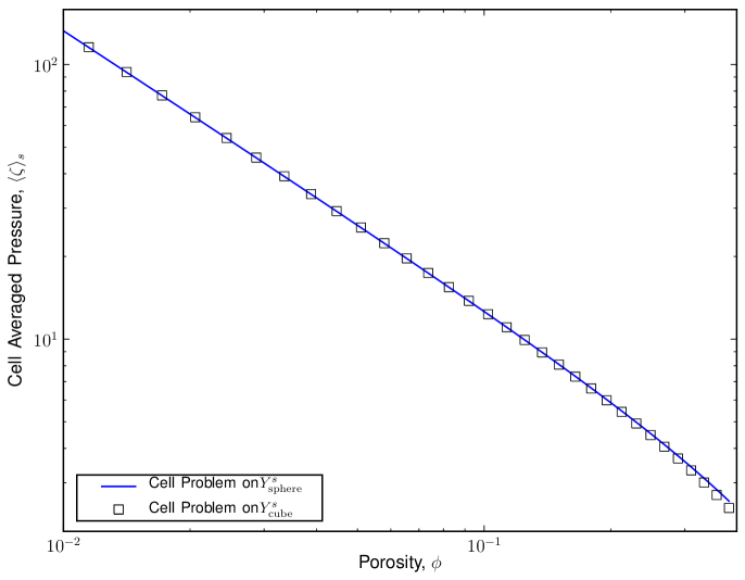
Figure 16: Cell averaged pressure, (41), plotted as a function of porosity. The data from the numerical solution of the cell problem given by equations (9a – 9c) and posed on ${Y_{s}}^{\textrm{cube}}$ also appears. It is in good agreement with the analytic solution on the spherical domain, ${Y_{s}}^{\textrm{sphere}}$.

Appendix B Computational Methods and Results

B.1 Cell Problem Boundary Conditions

Though we could solve the cell problems as stated, with the specified boundary conditions on interface $\gamma$ and periodic on the rest of the domain, we use the symmetry of our model problems to reduce the computational cost by a factor of eight. The symmetry properties of the solutions allow us to formulate the appropriate boundary conditions on the portion of the boundary that is not $\gamma$. The symmetry properties of the cell problems are summarized in Table 5. We specify these Dirichlet boundary conditions on the velocity together with the original boundary condition on $\gamma$. When forming the weak form of the problem, we use neutral boundary conditions, $\sigma\cdot\mathbf{n}=0$ on the part of the boundary that is not $\gamma$. For example, in solving the permeability cell problem of Section 3.1 for $\mathbf{k}^{1}$ and $q_{1}$, the weak form is

$$\int_{Y_{f}}\nabla\mathbf{k}^{1}:\nabla\bar{\phi}-q_{1}\nabla\cdot\bar{\phi}-\psi\nabla\cdot\mathbf{k}^{1}=\int_{Y_{f}}\bar{\phi}\cdot\mathbf{e}_{1}$$ (43)

where $\bar{\phi}$ and $\psi$ are test functions. The Dirichlet boundary conditions are indicated in Figure 17. On the part of the boundary that is the interface, $\gamma$, we have applied the no - slip condition.

Table 5: Summary of symmetry conditions used as Dirichlet boundary conditions in the cell problem computations.

Cell Problem Velocity	$y_{1}=0,-.5$	$y_{2}=0,-.5$	$y_{3}=0,-.5$
$\mathbf{k}^{1}$	$\mathbf{k}^{1}_{2}=\mathbf{k}^{1}_{3}=0$	$\mathbf{k}^{1}_{2}=0$	$\mathbf{k}^{1}_{3}=0$
$\bar{\chi}^{11}$	$\bar{\chi}_{1}^{11}=0$	$\bar{\chi}_{2}^{11}=0$	$\bar{\chi}_{3}^{11}=0$
$\bar{\chi}^{12}$	$\bar{\chi}_{2}^{12},\bar{\chi}_{3}^{12}=0$	$\bar{\chi}_{1}^{12}=\bar{\chi}_{3}^{12}=0$	$\bar{\chi}_{3}^{12}=0$
$\bar{\xi}$	$\bar{\xi}_{1}=0$	$\bar{\xi}_{2}=0$	$\bar{\xi}_{3}=0$

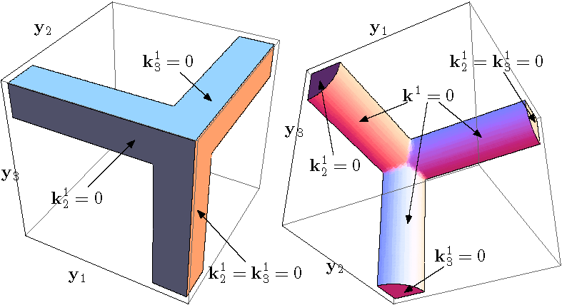
Figure 17: Specification of Dirichlet boundary conditions on $\mathbf{k}^{1}$ when solving on a symmetry reduced domain.

B.2 Solver Algorithms

We discretize the Stokes equations for the cell problems using the P2-P1 formulation described in [Elman et al.(2005)Elman, Silvester, and Wathen]. The FEniCS libraries are used to generate code for the weak forms of the equations and assemble the associated matrices and vectors, [Dupont et al.(2003)Dupont, Hoffman, Johnson, Kirby, Larson, Logg, and Scott, Kirby and Logg(2006), Kirby and Logg(2007), Logg(2007)]. These vectors and matrices are passed to PETSc and solved using algebraic Multigrid preconditioned GMRES, [Balay et al.(1997)Balay, Gropp, McInnes, and Smith, Balay et al.(2004)Balay, Buschelman, Eijkhout, Gropp, Kaushik, Knepley, McInnes, Smith, and Zhang, Balay et al.(2001)Balay, Buschelman, Gropp, Kaushik, Knepley, McInnes, Smith, and Zhang]. Domains and meshes were created with CUBIT [Sandia Corporation(2008)]. The versions of the software we used are summarized in Table 6.

Table 6: Software versions

Package	Version
CUBIT	11.0
DOLFIN(FEniCS)	0.7.2
FFC(FEniCS)	0.4.4
FIAT(FEniCS)	0.3.4
HYPRE	2.0.0
PETSc	2.3.3
UFC(FEniCS)	1.1
UMFPACK	4.3

To study problems with $O(10,000-100,000)$ elements and $O(100,000-1,000,000)$ unknowns, we rely on a Stokes preconditioner employing the pressure mass matrix of [Elman et al.(2005)Elman, Silvester, and Wathen]. The Stokes system is

$$\begin{pmatrix}\mathbb{A}&\mathbb{B}^{T}\\ \mathbb{B}&\mathbb{0}\end{pmatrix}\begin{bmatrix}\mathbb{u}\\ \mathbb{p}\end{bmatrix}=\mathbb{K}\begin{bmatrix}\mathbb{u}\\ \mathbb{p}\end{bmatrix}=\begin{bmatrix}\mathbb{f}\\ \mathbb{g}\end{bmatrix}$$

where $\mathbf{A}$ is matrix corresponding to the weak form of the vector Laplacian, $\mathbf{B}^{T}$ is the matrix corresponding to the weak form of the gradient, and $\mathbf{B}$ is the matrix corresponding to the weak form of the divergence. This is preconditioned with an approximate inverse of

$$\mathbb{P}=\begin{pmatrix}\mathbb{A}&\mathbb{0}\\ \mathbb{0}&\mathbb{Q}\end{pmatrix}$$

$\mathbb{Q}$ is the pressure-mass matrix.

As our meshes are unstructured, the HYPRE library is used for algebraic multigrid preconditioning. In particular, we use BoomerAMG. We apply this on all of $\mathbb{P}$, although we could have only used this on the $\mathbb{A}$ block, and relied on Jacobi or another light weight pre-conditioner for the $\mathbb{Q}$ block.

B.3 Examples and Benchmarks

As a test, we solve the permeability cell problem of Section 3.1, with the symmetry reductions, for flow past a sphere of radius $0.3$. It is meshed with a characteristic size of $.03125$, consisting of 119317 tetrahedrons. The results are summarized in Table 7

Table 7: Convergence comparison between solvers

Method	$\langle\mathbf{k}_{1}^{1}\rangle$
BoomerAMG on $\mathbb{P}$ + GMRES	0.0447051
JT05	0.045803
COMSOL	0.044497

For comparison, [Jung and Torquato(2005)] ran a time dependent problem to steady state and used an immersed boundary method with finite volumes. In our COMSOL computation, we used “fine” meshing, with 29649 elements, 134260 degrees of freedom, and a relative tolerance of 1e-10 in the solver.

The objective function, $\langle\mathbf{k}_{1}^{1}\rangle$, converges as we refine our mesh; see Table 8 for a comparison of different meshes for this problem.

Table 8: Convergence data for permeability cell problem I

Mesh Size	No. Cells	No. d.o.f.	$\langle\mathbf{k}_{1}^{1}\rangle_{f}$	$\left|\%\Delta\right|$
0.25	56	430	0.0492875	–
0.125	534	2950	0.0472207	0.0419336
0.0625	3673	17988	0.0452142	0.042492
0.03125	26147	119317	0.0447051	0.0112597
auto	14803	70525	0.0445419	–

Table 9 summarizes the convergence results for flow around a sphere of radius $0.45$. Again, our method appears to be quite effective.

Table 9: Convergence data for permeability cell problem II

Mesh Size	No. Cells	No. d.o.f.	$\langle\mathbf{k}_{1}^{1}\rangle_{f}$	$\left|\%\Delta\right|$
0.25	61	475	0.00763404	–
0.125	384	2302	0.00651896	0.146067
0.0625	2620	13370	0.00626809	0.0384831
0.03125	19916	93011	0.00617889	0.0142308
auto	23776	112620	0.00616139	–
JT05	–	–	0.0064803	–
COMSOL	–	–	0.006153	–

As another example, we solve the dilation stress cell problem from Section 3.2 . Solved on the domain complementary to a spherical inclusion of radius $0.2$, the convergence results are summarized in Table 10.

Table 10: Convergence data for dilation stress cell problem

Mesh Size	No. Cells	No. d.o.f.	$\langle\zeta\rangle_{s}$	$\left|\%\Delta\right|$
0.25	73	541	46.6432	–
0.125	514	2862	44.1747	0.052923
0.0625	3813	18575	40.7177	0.0782575
0.03125	29063	132115	39.4805	0.0303848
auto	13725	64205	39.1558	–
COMSOL	–	–	39.117074	–

The data in Tables 8– 10 were computed with default PETSc KSP tolerances. The automatically generated mesh was constructed with the CUBIT command:

volume 6 sizing function type skeleton scale 3 time_accuracy_level 2
min_size auto max_size 0.2 max_gradient 1.3

While these convergence results are encouraging, our data is imperfect. Continuing with the dilation stress example, consider the data in Figure 18. Comparing Figures (a), (c), and (e), it would appear that the domains with smaller fluid inclusions have less well resolved pressure fields. They could likely be resolved with additional resolution. However, we use this data and believe it to be valid for several reasons:

1. It is preferable to have all domains meshed with the same algorithm.

2. While the pressure fields may not be resolved, the error appears at the interface, and we are interested in the cell average. Moreover, the relative variations about the cell average are small.

3. The corresponding velocity fields, with magnitudes pictured in Figures (b), (d), and (f), appear to be smooth, suggesting we are converging towards the analytical solution.

4. The cell averages are consistent with the trends from the better resolved cases.

$\begin{array}[]{cc}\includegraphics[width=180.67499pt]{Figures/p40}&\includegraphics[width=180.67499pt]{Figures/v40}\\ \text{{(a)}}&\text{{(b)}}\\ \includegraphics[width=180.67499pt]{Figures/p20}&\includegraphics[width=180.67499pt]{Figures/v20}\\ \text{{(c)}}&\text{{(d)}}\\ \includegraphics[width=180.67499pt]{Figures/p10}&\includegraphics[width=180.67499pt]{Figures/v10}\\ \text{{(e)}}&\text{{(f)}}\end{array}$

Figure 18: Figures on the left are the pressure fields for domains complementing spheres of radii $a=.40$, $a=.20$, and $a=.10$. Figures on the right are the corresponding velocity magnitude fields.

B.4 Cell Problem Data

All meshes were generated using CUBIT with the command:

volume 6 sizing function type skeleton scale 3 time_accuracy_level 2
min_size auto max_size 0.2 max_gradient 1.3

Problems were solved in PETSc with a relative tolerance of $10^{-8}$ and and absolute tolerance of $10^{-50}$.