Metastability for Non-Linear Random Perturbations of Dynamical Systems

Abstract

In this paper we describe the long time behavior of solutions to quasi-linear parabolic equations with a small parameter at the second order term and the long time behavior of the corresponding diffusion processes.

2000 Mathematics Subject Classification Numbers: 60F10, 35K55.

Keywords: Nonlinear Perturbations, Metastability.

1 Introduction

Consider a dynamical system

$$\dot{X}^{x}_{t}=b(X^{x}_{t}),~{}~{}X^{x}_{0}=x\in\mathbb{R}^{d},$$ (1)

together with its stochastic perturbations

$$dX^{x,\varepsilon}_{t}=b(X^{x,\varepsilon}_{t})dt+\varepsilon\sigma(X^{x,\varepsilon}_{t})dW_{t},~{}~{}X^{x,\varepsilon}_{0}=x\in\mathbb{R}^{d}.$$ (2)

Here $\varepsilon>0$ is a small parameter, $W_{t}$ is a Wiener process in $\mathbb{R}^{d}$, and the coefficients $\sigma$ and $b$ are assumed to be Lipschitz continuous. The diffusion matrix $a(x)=(a_{ij}(x))=\sigma(x)\sigma^{*}(x)$ is assumed to be uniformly positive definite.

Together with (2), we can consider the corresponding Cauchy problem

$$\frac{\partial u^{\varepsilon}(t,x)}{\partial t}=L^{\varepsilon}u^{\varepsilon}:=\frac{\varepsilon^{2}}{2}\sum_{i,j=1}^{d}a_{ij}(x)\frac{\partial^{2}u^{\varepsilon}(t,x)}{\partial x_{i}\partial x_{j}}+b(x)\cdot\nabla_{x}u^{\varepsilon}(t,x),~{}~{}x\in\mathbb{R}^{d},~{}~{}t>0,$$ (3)

$$u^{\varepsilon}(0,x)=g(x),~{}x\in\mathbb{R}^{d},$$ (4)

where $g$ is a bounded continuous function.

Suppose for a moment that the vector field $b$ has just one asymptotically stable equilibrium point $O$ such that all the points get attracted to $O$ and $(b(x),x-O)\leq-c|x-O|$ for some positive constant $c$ and all sufficiently large $|x|$. Then it is easy to check that

$$\lim_{(\varepsilon,t)\rightarrow(0,\infty)}\mathrm{P}(X^{x,\varepsilon}_{t}\in U)=1$$

for any neighborhood $U$ of the equilibrium $O$. Taking into account that the solution $u^{\varepsilon}$ of (3)-(4) can be written in the form $u^{\varepsilon}(t,x)=\mathrm{E}g(X^{x,\varepsilon}_{t})$ and the continuity of $g$, we conclude that

$$\lim_{(\varepsilon,t)\rightarrow(0,\infty)}u^{\varepsilon}(t,x)=g(O).$$

A similar result holds in the case of a unique compact global attractor if the system (1) has a unique normalized invariant measure on the attractor. This is the case, for example, if the system (1) in $\mathbb{R}^{2}$ has a unique limit cycle attracting all the trajectories except the unstable equilibrium inside the cycle.

The situation becomes more complicated if the dynamical system has more than one asymptotically stable attractor. Assume, for brevity, that all the attractors are equilibriums $O_{1},...,O_{n}$. Let $D_{i}$ be the basin of $O_{i}$, $1\leq i\leq n$, and assume that the set $\mathbb{R}^{d}\setminus(D_{1}\cup...\cup D_{n})$ belongs to a finite union of surfaces of dimension $d-1$. The long time behavior of $X^{x,\varepsilon}_{t}$ and $u^{\varepsilon}(t,x)$ is now determined by the transitions of $X^{x,\varepsilon}_{t}$ between the attractors $O_{1},...,O_{n}$. These transitions are described by the large deviation theory for stochastic perturbations of dynamical systems developed in the late 1960-s (see [9] and references there). In particular, the weak limit $\mu$ of the invariant measure $\mu^{\varepsilon}$ of the family of processes (2) was found. In the generic case, the limiting measure $\mu$ is concentrated on one of the attractors, which will be denoted by $O^{*}$. Then

$$\lim_{\varepsilon\downarrow 0}\lim_{t\rightarrow\infty}u^{\varepsilon}(t,x)=g(O^{*}).$$

However, in the case of many attractors, the limiting behavior of $X^{x,\varepsilon}_{t}$ and $u^{\varepsilon}(t,x)$ as $\varepsilon\downarrow 0$ and $t\rightarrow\infty$ depends on the way in which $(\varepsilon,t)$ approaches $(0,\infty)$. Roughly speaking, under natural additional assumptions, there exist a finite number of regions in the neighborhood of $(0,\infty)$ such that the limiting distribution of $X^{x,\varepsilon}_{t}$ and the limit of $u^{\varepsilon}(t,x)$ exist if $(\varepsilon,t)$ approaches $(0,\infty)$ while staying inside one region. For different regions, these limits are, in general, different.

The corresponding theory of metastability (of sublimiting distributions) was developed in [4] (see also [6], [9], [12]). The notion of a hierarchy of cycles, which is discussed below, was introduced there. Let $S_{0,T}(\varphi)$ be the action functional for the family $X^{x,\varepsilon}_{t}$ in $C([0,T],\mathbb{R}^{d})$ as $\varepsilon\downarrow 0$ ([9]):

$$S_{0,T}(\varphi)=\frac{1}{2}\int_{0}^{T}\sum_{i,j=1}^{d}a^{ij}(\varphi_{t})(\dot{\varphi}^{i}_{t}-b_{i}(\varphi_{t}))(\dot{\varphi}^{j}_{t}-b_{j}(\varphi_{t}))dt,~{}~{}T\geq 0,~{}\varphi\in C([0,T],\mathbb{R}^{d})$$

for absolutely continuous $\varphi$, $S_{0,T}(\varphi)=+\infty$ for $\varphi$ that are not absolutely continuous. Here $a^{ij}$ are the elements of the inverse matrix, that is $a^{ij}=(a^{-1})_{ij}$. The quasi-potential is defined as

$$V(x,y)=\inf_{T,\varphi}\{S_{0,T}(\varphi):\varphi\in C([0,T],\mathbb{R}^{d}),\varphi(0)=x,\varphi(T)=y\},~{}~{}x,y\in\mathbb{R}^{d}.$$

Note that while the term “quasi-potential” is normally applied to the function $V$ of the variable $y$ with $x$ being a fixed equilibrium point, we use the same term for the function of two variables. The hierarchy of cycles is determined by the numbers

$$V_{ij}=V(O_{i},O_{j}),~{}~{}1\leq i,j\leq n.$$

The equilibriums $O_{1},...,O_{n}$ are the cycles of rank zero. In the generic case, for each $O_{i}$ there exists a unique “next” equilibrium $O_{l}=\mathcal{N}(O_{i})$ defined by $V_{il}=\min_{k:k\neq i}V_{ik}$. For each sufficiently small $\delta>0$, with probability close to one as $\varepsilon\downarrow 0$, the process $X^{x,\varepsilon}_{t}$ that starts in a $\delta$-neighborhood of $O_{i}$ will enter a $\delta$-neighborhood of $\mathcal{N}(O_{i})$ before visiting the basins of any of the equilibriums other than $O_{i}$ and $\mathcal{N}(O_{i})$. The time before the process enters the neighborhood of $O_{l}=\mathcal{N}(O_{i})$ is logarithmically equivalent to $\exp(V_{il}/\varepsilon^{2})$. If the sequence $O_{i}$, $\mathcal{N}(O_{i})$, $\mathcal{N}^{2}(O_{i})=\mathcal{N}(\mathcal{N}(O_{i})),...,\mathcal{N}^{n}(O_{i}),...$ is periodic, that is $\mathcal{N}^{n}(O_{i})=O_{i}$ for some $n$, then a cycle of rank one appears. It contains the cycles of rank zero $O_{i},\mathcal{N}(O_{i}),...,\mathcal{N}^{n-1}(O_{i})$. If $\mathcal{N}^{n}(O_{i})\neq O_{i}$ for any $n\geq 1$, we say that $O_{i}$ forms a cycle of rank one. The entire set of equilibriums is decomposed into cycles of rank one, which will be denoted by $C^{1}_{1},...,C^{1}_{m_{1}}$. Note that some of the cycles of rank one may consist of one cycle of rank zero.

Next, the transitions between cycles of rank one can be considered. Namely, in the generic case, for each cycle $C^{1}_{i}$ there is a different cycle $\mathcal{N}(C^{1}_{i})$ of rank one determined by $V_{ij}$, $1\leq i,j\leq n$, with the following property: if the process starts at one of the equilibrium points in $C^{1}_{i}$, then, with probability close to one as $\varepsilon\downarrow 0$, it will enter a $\delta$-neighborhood of one of the equilibrium points inside the cycle $\mathcal{N}(C^{1}_{i})$ before visiting basins of any of the equilibriums outside $C^{1}_{i}$ and $\mathcal{N}(C^{1}_{i})$. This leads to the decomposition of the set of cycles or rank one into cycles of rank two.

This procedure can be continued inductively until we arrive at a single cycle of finite rank $R$ which contains all the equilibrium points. The cycles of rank $r\leq R$ will be denoted by $C^{r}_{1},...,C^{r}_{m_{r}}$.

Let $T^{\varepsilon}(\lambda)=\exp(\lambda/\varepsilon^{2})$. (The results stated in the paper also hold for $T^{\varepsilon}(\lambda)\asymp\exp(\lambda/\varepsilon^{2})$, that is if $\varepsilon^{2}\ln T^{\varepsilon}(\lambda)\rightarrow\lambda$ as $\varepsilon\downarrow 0$.) In the generic case, there is a finite set $\Lambda\subset(0,\infty)$ such that for each $x\in D_{1}\cup...\cup D_{n}$ and each $\lambda\in(0,\infty)\setminus\Lambda$, one equilibrium $O_{M(x,\lambda)}$ is defined such that the measures $\mu^{\varepsilon}(\Gamma)=\mathrm{P}(X^{x,\varepsilon}_{T^{\varepsilon}(\lambda)}\in\Gamma)$ converge weakly to the $\delta$-measure concentrated at $O_{M(x,\lambda)}$. The state $O_{M(x,\lambda)}$ is called the metastable state for the initial point $x$ and the time scale $T^{\varepsilon}(\lambda)$.

In this paper, instead of the linear problem (3)-(4), we will consider the Cauchy problem for the quasi-linear equation with a small parameter

$$\frac{\partial u^{\varepsilon}(t,x)}{\partial t}=L^{\varepsilon}u^{\varepsilon}:=\frac{\varepsilon^{2}}{2}\sum_{i,j=1}^{d}a_{ij}(x,u^{\varepsilon})\frac{\partial^{2}u^{\varepsilon}(t,x)}{\partial x_{i}\partial x_{j}}+b(x)\cdot\nabla_{x}u^{\varepsilon}(t,x),~{}~{}x\in\mathbb{R}^{d},~{}~{}t>0,$$ (5)

$$u^{\varepsilon}(0,x)=g(x),~{}x\in\mathbb{R}^{d}.$$ (6)

Equations with diffusion coefficients depending on particle concentration arise naturally in many applications, in particular in population genetics. The situation when the drift $b$ depends on both $x$ and $u^{\varepsilon}$, with certain additional assumptions, can also be considered, but we assume here that $b$ depends only on $x$ for the sake of simplicity.

We assume that the coefficients of equation (5) are Lipschitz continuous and bounded; the matrix $(a_{ij}(x,u))$ is assumed to be uniformly positive definite. Under these conditions, problem (5)-(6) has a unique solution for any continuous bounded $g(x)$ (see, for instance, [11]).

A family of processes $X^{x,\varepsilon}_{t}$, $x\in\mathbb{R}^{d}$, satisfying equation (2) corresponds to each linear operator $L^{\varepsilon}$ defined by (3). In the nonlinear case, a family of processes corresponds to the initial value problem (5)-(6). Namely, taking into account the representation of the solution of the (linear) Cauchy problem as the expected value of an appropriate functional of the process, the family corresponding to the problem (5)-(6) is defined by the following system (see [5], Ch. 5):

$$dX^{t,x,\varepsilon}_{s}=b(X^{t,x,\varepsilon}_{s})ds+\varepsilon\sigma(X^{t,x,\varepsilon}_{s},u^{\varepsilon}(t-s,X^{t,x,\varepsilon}_{s}))dW_{s},~{}~{}s\leq t,~{}~{}~{}X^{t,x,\varepsilon}_{0}=x,$$ (7)

$$u^{\varepsilon}(t,x)=\mathrm{E}g(X^{t,x,\varepsilon}_{t}),$$ (8)

where the entries $\sigma_{ij}$ of the matrix $\sigma(x,u)$ are Lipschitz continuous and $\sigma\sigma^{*}=a$. The process $X^{t,x,\varepsilon}_{s}$ can be viewed as a nonlinear stochastic perturbation of the dynamical system (1).

Under the above assumptions on the coefficients and the function $g$, the solution of the system (7)-(8) exists and is unique. The first initial-boundary value problem for quasi-linear parabolic equation with a small diffusion and the exit problem for the corresponding processes were studied in [7]. The results of the latter paper will be used here.

While the action functional and the quasi-potential were determined by the time-independent coefficients in the linear case, now we will consider a family of action functionals and corresponding quasi-potentials $V_{ij}(c(\lambda))$, $\lambda>0$. These will be used for times of order $T^{\varepsilon}(\lambda)=\exp(\lambda/\varepsilon^{2})$. Namely, we will show that the solution $u^{\varepsilon}$ of (5), in the time scale $T^{\varepsilon}(\lambda)$, is very close to a constant $c(\lambda)$ inside $D_{i}$. We can then define the action functionals and $V_{ij}(c(\lambda))$ as in the linear case by substituting the constant $c(\lambda)$ for the second argument in the diffusion coefficient in the equation.

The main difficulty is that now the action functional and quasi-potential evolve in time due their dependence on the (unknown) solution $u^{\varepsilon}$. Consider, however, a time interval $[T^{\varepsilon}(\lambda-\delta),T^{\varepsilon}(\lambda)]$, where $\delta$ is small. As will be seen, $u^{\varepsilon}$ typically does not change much in time on this time interval, and the large deviation theory still applies without drastic modifications, which allows us to express the limit of $u^{\varepsilon}(T^{\varepsilon}(\lambda),x)$, as $\varepsilon\downarrow 0$, in terms of the limit of $u^{\varepsilon}(T^{\varepsilon}(\lambda-\delta),x)$ and the functions $V_{ij}(c(\lambda))$. This is the main idea which will allow us to study the evolution in $\lambda$ of the limit of $u^{\varepsilon}(T^{\varepsilon}(\lambda),x)$. This, in turn, provides a description of the behavior of $X^{T^{\varepsilon}(\lambda),x,\varepsilon}_{s}$ as $\varepsilon\downarrow 0$.

We will show that if $\lambda$ is sufficiently large, then the distribution of $X^{T^{\varepsilon}(\lambda),x,\varepsilon}_{T^{\varepsilon}(\lambda)}$, even in a generic case, converges not necessarily to a $\delta$-measure concentrated at an equilibrium point, but to a distribution on the set of equilibrium points. Under some natural assumptions this happens, for example, in the case of two equilibrium points if $V_{12}(c)=V_{21}(c)$ for some value of $c$. Therefore, in the case of nonlinear perturbations, the notion of a metastable state should be replaced by the notion of a metastable distribution.

Note that metastable distributions (rather than states) arise also in the case of linear parabolic equations. For example, if the non-perturbed system, say in $\mathbb{R}^{2}$, has two asymptotically stable limit cycles attracting the entire space, other than the separatrices, then each of the invariant distributions on those cycles will be the metastable distribution for the appropriate initial states and time scales. Metastable distributions on an asymptotically stable attractor arise in physical models (see various models and references in [12]). However, in the case considered here, the metastable distributions are supported on several separated asymptotically stable attractors. Similar metastable distributions arise also when perturbations of nearly-Hamiltonian systems are considered (see [1], [3]), but because of different reasons.

Since the quasi-potential changes in time, the relative stability of attractors also changes in time, possibly leading to changes in the hierarchy of cycles. We will mostly be concerned with the situation when the hierarchy of cycles does not change. This is the case, for example, if there are only two equilibrium points or if the matrix $a_{ij}(x,u)$ is close enough to a diffusion matrix independent of $u$. An example with a change in the hierarchy of cycles is considered in Section 6.

If the system has $n$ asymptotically stable equilibrium points (or more general stable attractors), the number of different (even generic) cases which should be considered grows very fast with $n$: one should consider not just different hierarchies of cycles, but also different relations between the values of the initial function $g$ at the equilibriums and various behaviors of $V_{ij}(c)$ as $c$ changes. Therefore we consider in more detail the case of two attractors and describe the result in the case of three attractors. The general result is not presented, but we believe that the methodology developed in this paper for the case of small $n$ works in general (generic) case.

In Section 2 we introduce some of the definitions and discuss the notion of the hierarchy of cycles in more detail. We also state the lemmas that can be used to describe the long-time behavior of a process whose time-dependent coefficients are close to functions that do not depend on time. In Sections 3 and 4 we consider a system with two equilibriums and a system with three equlibriums on the real line in the case when the hierarchy of cycles is preserved. In Section 5 we formulate a general result for the case when the hierarchy of cycles is preserved. In Section 6 we study the asymptotics of the solution to the parabolic equation for a system in which a bifurcation in the hierarchy of cycles occurs.

2 Notations. Diffusion Processes Corresponding to the Nonlinear Problem

Let $\alpha(x)$ be a symmetric $d\times d$ matrix whose elements $\alpha_{ij}(x)$ are Lipschitz continuous with Lipschitz constant $L$ and satisfy

$$k|\xi|^{2}\leq\sum_{i,j=1}^{d}\alpha_{ij}(x)\xi_{i}\xi_{j}\leq K|\xi|^{2},~{}~{}x\in\mathbb{R}^{d},~{}~{}\xi\in\mathbb{R}^{d}.$$ (9)

Let $\alpha^{ij}$ be the elements of the inverse matrix, that is $\alpha^{ij}=(\alpha^{-1})_{ij}$, and $\sigma$ be a square matrix such that $\alpha=\sigma\sigma^{*}$. We choose $\sigma$ in such a way that $\sigma_{ij}$ are also Lipschitz continuous.

We assume that all the attractors of the bounded Lipschitz continuous vector field $b$ are equilibriums $O_{1},...,O_{n}$. Assume that their domains of attraction $D_{1},...,D_{n}$ are such that the set $\mathbb{R}^{d}\setminus(D_{1}\cup...\cup D_{n})$ belongs to a finite union of surfaces of dimension $d-1$. We also assume that there are $r>0$ and $c>0$ such that

$$(b(x),x-O_{i})\leq-c|x-O_{i}|^{2}$$ (10)

whenever $x$ is in the $r$-neighborhood of $O_{i}$, $1\leq i\leq n$.

Let $S^{\alpha}_{0,T}$ be the normalized action functional for the family of processes $X^{x,\varepsilon}_{t}$ satisfying

$$dX^{x,\varepsilon}_{t}=b(X^{x,\varepsilon}_{t})dt+\varepsilon\sigma(X^{x,\varepsilon}_{t})dW_{t},~{}~{}X^{x,\varepsilon}_{0}=x,$$ (11)

where $b$ is a bounded Lipschitz continuous vector field on $\mathbb{R}^{d}$. Thus

$$S^{\alpha}_{0,T}(\varphi)=\frac{1}{2}\int_{0}^{T}\sum_{i,j=1}^{d}\alpha^{ij}(\varphi_{t})(\dot{\varphi}^{i}_{t}-b_{i}(\varphi_{t}))(\dot{\varphi}^{j}_{t}-b_{j}(\varphi_{t}))dt$$

for absolutely continuous $\varphi$ defined on $[0,T]$, $\varphi_{0}=x$, and $S^{\alpha}_{0,T}(\varphi)=\infty$ if $\varphi$ is not absolutely continuous or if $\varphi_{0}\neq x$ (see [9]). Let $V^{\alpha}(x,y)$ be the quasi-potential for the family $X^{x,\varepsilon}_{t}$ in $\mathbb{R}^{d}$, that is

$$V^{\alpha}(x,y)=\inf_{T,\varphi}\{S^{\alpha}_{0,T}(\varphi):\varphi\in C([0,T],\mathbb{R}^{d}),\varphi(0)=x,\varphi(T)=y\},~{}~{}x,y\in\mathbb{R}^{d}.$$ (12)

Let $V^{\alpha}_{ij}=V^{\alpha}(O_{i},O_{j})$. For a given function $\alpha$, we define inductively the following objects (see [4], [9] for a detailed exposition).

(a) The hierarchy of cycles $C^{r}_{1},...,C^{r}_{m_{r}}$, $r\leq R$.

(b) The notion of the “next” equilibrium $\nu(C^{r}_{i})$ and the “next” cycle $\mathcal{N}(C^{r}_{i})$ of the same rank for a cycle $C^{r}_{i}$ of rank less than $R$.

(c) The transition rates $V^{\alpha}_{C^{r}_{i},O_{j}}$, $1\leq i\leq m_{r}$, $1\leq j\leq n$, $O_{j}\notin C^{r}_{i}$, from a cycle to equilibriums outside this cycle.

For $r=0$, we define $C^{0}_{i}=\{O_{i}\}$, $V^{\alpha}_{C^{0}_{i},O_{j}}=V^{\alpha}_{ij}$. Assume that the cycles of rank $r$ and the transition rates from those cycles to equilibrium points have been defined. We define $O_{j}$ to be the next equilibrium after $C^{r}_{i}$ if $\min_{j:O_{j}\notin C^{r}_{i}}V^{\alpha}_{C^{r}_{i},O_{j}}$ is achieved at $j$.

Assumption A. The minimum $\min_{j:O_{j}\notin C^{r}_{i}}V^{\alpha}_{C^{r}_{i},O_{j}}$ is achieved for a single value of $j$.

We will write $O_{j}=\nu(C^{r}_{i})$ to express that $O_{j}$ is the next equilibrium after $C^{r}_{i}$. We say that the cycle $C^{r}_{l}$ of rank $r$ is the next after $C^{r}_{i}$ if $C^{r}_{l}$ contains $\nu(C^{r}_{i})$. We will express this relation by writing $C^{r}_{l}=\mathcal{N}(C^{r}_{i})$. Starting from a cycle $C^{r}_{i}$ of rank $r$, we can form the sequence $C^{r}_{i},\mathcal{N}(C^{r}_{i}),\mathcal{N}^{2}(C^{r}_{i}),...$ by using the operation “next”. If this sequence is periodic, that is $C^{r}_{i}=\mathcal{N}^{n}(C^{r}_{i})$ for some $n$, then the cycles $C^{r}_{i},...,\mathcal{N}^{n-1}(C^{r}_{i})$ form a cycle of rank $r+1$. If $C^{r}_{i}\neq\mathcal{N}^{n}(C^{r}_{i})$ for any $n\geq 1$, then $C^{r}_{i}$ is said to form a cycle of rank $r+1$. This way, the collection of all the cycles of rank $r$ is decomposed in a union of non-intersecting cycles of rank $r+1$.

If $C^{r}_{1},...,C^{r}_{s}$ form a cycle of rank $r+1$, which will be denoted by $\Gamma$, we define $V^{\alpha}_{\Gamma,O_{j}}$ as

$$V^{\alpha}_{\Gamma,O_{j}}=\max_{1\leq m\leq s}V^{\alpha}_{C^{r}_{m},\nu(C^{r}_{m})}+\min_{1\leq m\leq s}(V^{\alpha}_{C^{r}_{m},O_{j}}-V^{\alpha}_{C^{r}_{m},\nu(C^{r}_{{m}})}),~{}~{}O_{j}\notin\Gamma.$$ (13)

We can continue this procedure until we arrive at a single cycle of highest rank $R$.

If $\Gamma$ is a cycle, we define $D_{\Gamma}=\cup_{i:O_{i}\in\Gamma}D_{i}$. As follows from [4], [9], if the process (11) starts in $D_{\Gamma}$, where $\Gamma$ is a cycle of rank $r<R$, then with probability which tends to one as $\varepsilon\downarrow 0$ it will leave $D_{\Gamma}$ and enter a small neighborhood of $\nu(\Gamma)$ in time $T(\varepsilon)\asymp\exp(V^{\alpha}_{\Gamma,\nu(\Gamma)}/\varepsilon^{2})$.

Next we discuss the long-time behavior of processes whose diffusion coefficients are time-dependent, but are close to functions that do not depend on time. For $T>0$ and $\varphi,\psi\in C([0,T],\mathbb{R}^{d})$, we define $\rho_{T}(\varphi,\psi)=\sup_{t\in[0,T]}|\varphi(t)-\psi(t)|$.

Let $\widetilde{\alpha}^{\varepsilon}(t,x)$ be a uniformly positive definite symmetric $d\times d$ matrix whose elements $\widetilde{\alpha}_{ij}^{\varepsilon}$ are continuous in $(t,x)$ and Lipschitz continuous in $x$. Let $\widetilde{\sigma}^{\varepsilon}$ be a square matrix such that $\widetilde{\alpha}^{\varepsilon}=\widetilde{\sigma}^{\varepsilon}(\widetilde{\sigma}^{\varepsilon})^{*}$. We choose $\widetilde{\sigma}^{\varepsilon}$ in such a way that $\widetilde{\sigma}_{ij}^{\varepsilon}$ are also continuous in $(t,x)$ and Lipschitz continuous in $x$.

Let $\widetilde{X}^{x,\varepsilon}_{t}$ satisfy $\widetilde{X}^{x,\varepsilon}_{0}=x$ and

$$d\widetilde{X}^{x,\varepsilon}_{t}=b(\widetilde{X}^{x,\varepsilon}_{t})dt+\varepsilon\widetilde{\sigma}^{\varepsilon}(t,\widetilde{X}^{x,\varepsilon}_{t})dW_{t},$$ (14)

where $b$ is the same as above. The law of this process depends on $\widetilde{\sigma}^{\varepsilon}$ only through $\widetilde{\alpha}^{\varepsilon}=\widetilde{\sigma}^{\varepsilon}(\widetilde{\sigma}^{\varepsilon})^{*}$. We will assume that the diffusion coefficients for the process $\widetilde{X}^{x,\varepsilon}_{t}$ are close to those of ${X}^{x,\varepsilon}_{t}$. Namely, let us assume that

$$\sup_{(t,x)\in\mathbb{R}^{+}\times\mathbb{R}^{d}}|\widetilde{\alpha}_{ij}^{\varepsilon}(t,x)-{\alpha}_{ij}(x)|\leq\varkappa,$$ (15)

where $\varkappa$ is small. The reason to introduce the process $\widetilde{X}^{x,\varepsilon}_{t}$ is that we would like to study the behavior of the process $X^{t,x,\varepsilon}_{s}$ given by (7)-(8) on a time interval where the variable $u^{\varepsilon}$ found inside the diffusion coefficient of (7) does not change much. Since a-priori we don’t know much about the behavior of the diffusion coefficients in (7) (other than that they don’t significantly change in time on a certain time interval), it is convenient to consider a generic process whose diffusion coefficients are close to functions that don’t depend on time.

The next two lemmas show that $S^{\alpha}$ serves a purpose similar to the action functional for the process $\widetilde{X}^{x,\varepsilon}_{t}$, even though the diffusion coefficients for the process are time-dependent.

Lemma 2.1.

Suppose that $b$ is fixed, $\alpha$ and $\widetilde{\alpha}^{\varepsilon}$ are as above, and positive constants $k$, $K$ and $L$ are fixed. For any $\delta$, $\gamma$ and $C$ there exist $\varkappa>0$ and $\varepsilon_{0}>0$ such that

$$\mathrm{P}(\rho_{T}(\widetilde{X}^{x,\varepsilon}_{t},\varphi)<\delta)\geq\exp(-\varepsilon^{-2}[S^{\alpha}_{0,T}(\varphi)+\gamma])$$

for $\varepsilon<\varepsilon_{0}$ and $T>0$, $\varphi\in C([0,T],\mathbb{R}^{d})$ such that $\varphi(0)=x$ and $T+S^{\alpha}_{0,T}(\varphi)<C$.

Lemma 2.2.

Suppose that $b$ is fixed, $\alpha$ and $\widetilde{\alpha}^{\varepsilon}$ are as above, and the positive constants $k$, $K$ and $L$ are fixed. For $x\in\mathbb{R}^{d}$, $T>0$ and $s\geq 0$, put

$$\Phi(s)=\{\varphi\in C([0,T],\mathbb{R}^{d}),\varphi(0)=x,S^{\alpha}_{0,T}(\varphi)\leq s\}.$$

For any $T>0$, $\delta>0$, $\gamma>0$ and $s_{0}>0$, there exist $\varkappa>0$ and $\varepsilon_{0}>0$ such that for $x\in\mathbb{R}^{d}$, $0<\varepsilon\leq\varepsilon_{0}$ and $s\leq s_{0}$, we have

$$\mathrm{P}(\rho_{T}(\widetilde{X}^{x,\varepsilon}_{t},\Phi(s))\geq\delta)\leq\exp(-\varepsilon^{-2}[s-\gamma]).$$

Note that the choice of $\varkappa$ and $\varepsilon_{0}$ in the above lemmas depends on $\alpha$ and $\widetilde{\alpha}^{\varepsilon}$ only through $k$, $K$ and $L$.

Sketch of the proof of Lemmas 2.1 and 2.2. The proof of these lemmas is similar to the proof of the fact that $S^{\alpha}_{0,T}(\varphi)$ serves as an action functional for the process $X^{x,\varepsilon}_{t}$ given in (11) (see [8], [2]). In order to apply the method based on the Euler approximations (see Section 1.4 of [2]), we need to show that a process with constant diffusion coefficients is close to a process with slightly perturbed coefficients in the following sense:

Let $Y^{x,\varepsilon}_{t}$, $\widetilde{Y}^{x,\varepsilon}_{t}$ satisfy

$$dY^{x,\varepsilon}_{t}=bdt+\varepsilon\sigma dW_{t},~{}~{}Y^{x,\varepsilon}_{0}=x,$$ (16)

$$d\widetilde{Y}^{x,\varepsilon}_{t}=bdt+\varepsilon(\sigma+\delta(t,\widetilde{Y}^{x,\varepsilon}_{t}))dW_{t},~{}~{}\widetilde{Y}^{x,\varepsilon}_{0}=x,$$ (17)

where $b$ is a constant vector, $\sigma$ is a constant matrix, and $\delta(t,x)$ is a matrix whose entries are continuous in $(t,x)$ and Lipschitz continuous in $x$. Then for each positive $h$, $A$ and $T$, there is a positive $\delta_{0}$ such that

$$\mathrm{P}(\sup_{t\leq T}|Y^{x,\varepsilon}_{t}-\widetilde{Y}^{x,\varepsilon}_{t}|>h)\leq\exp(-A/(\varepsilon^{2}T))$$ (18)

if $\sup_{t,x}||\delta(t,x)||\leq\delta_{0}$ and $\varepsilon$ is sufficiently small. (Here we define $||\delta||=\sqrt{\sum_{i,j=1}^{d}(\delta^{ij})^{2}}~{}$). To prove (18), we note that the $i$-th component of the difference satisfies

$$M^{i}_{t}:=(Y^{x,\varepsilon}_{t}-\widetilde{Y}^{x,\varepsilon}_{t})^{i}=\varepsilon\int_{0}^{t}\sum_{j=1}^{d}\delta^{ij}(t,\widetilde{Y}^{x,\varepsilon}_{s}))dW^{j}_{s}.$$

The right hand side is a martingale with quadratic variation satisfying

$$\langle M^{i}\rangle_{t}\leq\varepsilon^{2}t\sup_{t,x}||\delta(t,x)||^{2}\leq\varepsilon^{2}t\delta_{0}^{2}.$$

Therefore

$$\sup_{t\leq T}|M^{i}_{t}|\leq\sup_{t\leq T}|\widetilde{W}(\varepsilon^{2}t\delta_{0}^{2})|,$$

where $\widetilde{W}$ is a standard Brownian motion. Therefore

$$\mathrm{P}(\sup_{t\leq T}|Y^{x,\varepsilon}_{t}-\widetilde{Y}^{x,\varepsilon}_{t}|>h)\leq d\mathrm{P}(\sup_{t\leq T}|\widetilde{W}(\varepsilon^{2}t\delta_{0}^{2})|>\frac{h}{d}),$$

which can clearly be made smaller than the right hand side of (18) by selecting a sufficiently small $\delta_{0}$. ∎

We next state a corollary of the above two lemmas that will be used in the paper. Given a domain $D$ and $\delta>0$, we define

$$D^{\delta}=\{x\in D:{\rm dist}(x,\partial D)\geq\delta,~{}|x|\leq 1/\delta\}.$$

Let $x_{0}$ be an asymptotically stable equilibrium of $b$ and $D$ be a domain attracted to $x_{0}$. Let

$$v=\inf_{T,\varphi}\{S^{\alpha}_{0,T}(\varphi):\varphi\in C([0,T],\overline{D}),\varphi(0)=x_{0},\varphi(T)\in\partial D\}.$$

Lemma 2.3.

Suppose that $b$ is fixed, $\alpha$ is Lipschitz continuous with Lipschitz constant $L$, $\widetilde{\alpha}^{\varepsilon}$ is continuous in $(t,x)$ and Lipschitz continuous in $x$, and

$$k|\xi|^{2}\leq\sum_{i,j=1}^{d}{\alpha}_{ij}(x)\xi_{i}\xi_{j}\leq K|\xi|^{2}~{}~{}for~{}~{}x\in D,~{}~{}\xi\in\mathbb{R}^{d},$$

$$k|\xi|^{2}\leq\sum_{i,j=1}^{d}\widetilde{\alpha}_{ij}^{\varepsilon}(t,x)\xi_{i}\xi_{j}\leq K|\xi|^{2}~{}~{}for~{}~{}(t,x)\in\mathbb{R}^{+}\times D,~{}~{}\xi\in\mathbb{R}^{d}.$$ (19)

For each $\delta>0$ there are $\varkappa>0$ and a function $\rho(\varepsilon)$ (that depend on $\alpha$ and $\widetilde{\alpha}$ through $L,k$ and $K$) such that $\lim_{\varepsilon\downarrow 0}\rho(\varepsilon)=0$ and

$$\sup_{(t,x)\in[T^{\varepsilon}(\delta),T^{\varepsilon}(v-\delta)]\times D^{\varkappa}}\mathrm{P}(|\widetilde{X}^{x,\varepsilon}_{t}-x_{0}|<\delta,~{}\widetilde{X}^{x,\varepsilon}_{s}\in D~{}~{}{\rm for}~{}~{}s\leq t)\geq 1-\rho(\varepsilon),$$

provided that

$$\sup_{(t,x)\in\mathbb{R}^{+}\times D^{\varkappa}}|\widetilde{\alpha}_{ij}^{\varepsilon}(t,x)-{\alpha}_{ij}(x)|\leq\varkappa.$$

This lemma can be easily proved using a modification of Theorems 4.2 and 4.3 from Chapter 4 of [9] if we substitute our Lemmas 2.1 and 2.2 for the corresponding results concerning the case of time-independent coefficients.

The next simple lemma does not require the proximity of $\widetilde{\alpha}^{\varepsilon}$ to $\alpha$, but only the boundedness of the entries of $\widetilde{\alpha}^{\varepsilon}$. It can be proved by standard arguments from large deviation theory (compare with chapter 3 of [9]).

Lemma 2.4.

Suppose that $b$ is fixed and $\widetilde{\alpha}^{\varepsilon}$ is continuous in $(t,x)$ and Lipschitz continuous in $x$ and satisfies (19). For any compact $M\subset D$, there is $v_{0}>0$ which depends on $\widetilde{\alpha}^{\varepsilon}$ only through $K$ such that for each $\delta\in(0,v_{0})$ there is a function $\rho(\varepsilon)$ such that $\lim_{\varepsilon\downarrow 0}\rho(\varepsilon)=0$ and

$$\sup_{(t,x)\in[T^{\varepsilon}(\delta),T^{\varepsilon}(v_{0})]\times M}\mathrm{P}(|\widetilde{X}^{x,\varepsilon}_{t}-x_{0}|<\delta,~{}\widetilde{X}^{x,\varepsilon}_{s}\in D~{}~{}{\rm for}~{}~{}s\leq t)\geq 1-\rho(\varepsilon).$$

Note that the quasi-potential can be defined by (12) even if $\alpha$ has some discontinuities. We shall be particularly interested in the structure of the hierarchy of cycles and the exponential transition times for functions $\alpha$ which are of the form $\alpha=a(x,f(x))$, where $f$ is constant on each $D_{i}$. The reason for that is that the solution of (5)-(6) is nearly constant inside each of the domains $D_{i}^{\delta}=\{x\in D_{i}:{\rm dist}(x,\partial D_{i})\geq\delta,~{}|x|\leq 1/\delta\}$, $\delta>0$, $1\leq i\leq n$, for $\varepsilon$ small enough, as follows from the following lemma.

Lemma 2.5.

Let $u^{\varepsilon}$ be the solution of (5)-(6). For every positive $\lambda_{0}$ and $\delta$ there is a positive $\varepsilon_{0}$ such that

$$|u^{\varepsilon}(T^{\varepsilon}(\lambda),x)-u^{\varepsilon}(T^{\varepsilon}(\lambda),O_{i})|\leq\delta$$ (20)

whenever $x\in D_{i}^{\delta}$, $\varepsilon\leq\varepsilon_{0}$ and $\lambda\geq\lambda_{0}$.

For a proof of this lemma we refer the reader to [7], where the same statement was proved in the case of a single domain.

3 The case of two equilibrium points

In this section we assume that there are two asymptotically stable equilibrium points $O_{1},O_{2}\in\mathbb{R}^{d}$. Let $D_{1}\subset\mathbb{R}^{d}$ be the set of points in $\mathbb{R}^{d}$ which are attracted to $O_{1}$ and $D_{2}\subset\mathbb{R}^{d}$ the set of points attracted to $O_{2}$. We assume that $D_{1}\cup D_{2}\in\mathbb{R}^{d}\setminus S$, where $S$ is a $(d-1)$-dimensional manifold. Note that in the case of two equilibrium points, the hierarchy of cycles is always the same: $O_{1}$ and $O_{2}$ are cycles of rank zero, and there is one cycle of rank one which contains both $O_{1}$ and $O_{2}$.

Let $g_{\rm min}=\inf_{x\in\mathbb{R}^{d}}g(x)$ and $g_{\rm max}=\sup_{x\in\mathbb{R}^{d}}g(x)$. Define the functions $M_{12}$, $M_{21}:[g_{\rm min},g_{\rm max}]\rightarrow\mathbb{R}$ via

$$M_{12}(c)={V}^{a(\cdot,c)}_{O_{1},O_{2}},~{}~{}M_{21}(c)={V}^{a(\cdot,c)}_{O_{2},O_{1}}.$$

These functions are shown on Figure 1. It is not difficult to check that the constant $c$ in the second argument of $a$ can be replaced by any function equal to $c$ on $D_{1}$ in the definition of $M_{12}$ and equal to $c$ on $D_{2}$ in the definition of $M_{21}$ without affecting the values of $M_{12}(c)$ and $M_{21}(c)$.

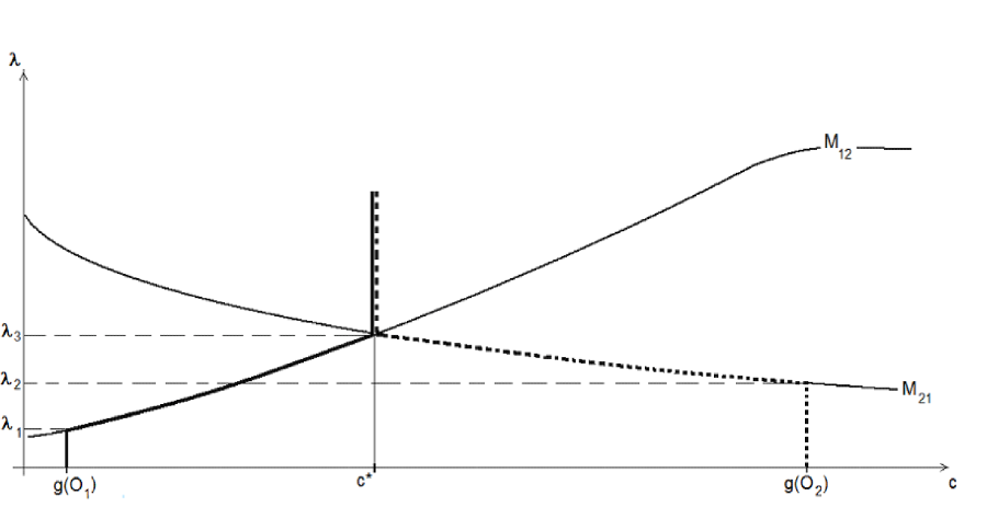
Figure 1: The case of two equilibrium points

Without loss of generality we may assume that $g(O_{1})\leq g(O_{2})$. Let $\lambda_{1}=M_{12}(g(O_{1}))$ and $\lambda_{2}=M_{21}(g(O_{2}))$. In order to formulate the results on the asymptotics of $u^{\varepsilon}(T^{\varepsilon}(\lambda),x)$, we need the functions $c^{1}(\lambda)$ and $c^{2}(\lambda)$, $\lambda>0$, defined as follows:

$$c^{1}(\lambda)=\left\{\begin{array}[]{lll}g(O_{1}),~{}~{}~{}~{}~{}~{}~{}~{}~{}~{}~{}~{}~{}~{}~{}~{}~{}~{}~{}~{}~{}~{}~{}~{}~{}~{}~{}~{}~{}~{}~{}~{}~{}~{}~{}~{}~{}~{}~{}~{}~{}~{}~{}~{}~{}~{}~{}~{}~{}~{}~{}~{}~{}~{}~{}~{}~{}~{}~{}~{}~{}~{}~{}\,0<\lambda<\lambda_{1},\\ \min\{g(O_{2}),\min\{c:c\in[g(O_{1}),g(O_{2})],M_{12}(c)=\lambda\}\},~{}~{}\,\,\lambda\geq\lambda_{1},\end{array}\right.$$ (21)

$$c^{2}(\lambda)=\left\{\begin{array}[]{lll}g(O_{2}),~{}~{}~{}~{}~{}~{}~{}~{}~{}~{}~{}~{}~{}~{}~{}~{}~{}~{}~{}~{}~{}~{}~{}~{}~{}~{}~{}~{}~{}~{}~{}~{}~{}~{}~{}~{}~{}~{}~{}~{}~{}~{}~{}~{}~{}~{}~{}~{}~{}~{}~{}~{}~{}~{}~{}~{}~{}~{}~{}~{}~{}~{}~{}~{}\,0<\lambda<\lambda_{2},\\ \max\{g(O_{1}),\max\{c:c\in[g(O_{1}),g(O_{2})],M_{21}(c)=\lambda\}\},~{}~{}\,\,\lambda\geq\lambda_{2}.\end{array}\right.$$ (22)

Let $\lambda_{3}=\inf\{\lambda:c^{1}(\lambda)\geq c^{2}(\lambda)\}$. Assume that at least one of the functions $c^{1}$ and $c^{2}$ is continuous at $\lambda_{3}$. Let $c^{*}=c^{1}(\lambda_{3})$ if $c^{1}$ is continuous at $\lambda_{3}$ and $c^{*}=c^{2}(\lambda_{3})$ otherwise. Let $\overline{c}^{1}(\lambda)=\min(c^{1}(\lambda),c^{*})$ and $\overline{c}^{2}(\lambda)=\max(c^{2}(\lambda),c^{*})$. On Figure 2, the graphs of $\overline{c}^{1}$ and $\overline{c}^{2}$ are denoted by the thick and the dotted lines, respectively.

The asymptotics of $u^{\varepsilon}(T^{\varepsilon}(\lambda),x)$ is described by the following theorem. Later, we will use this result to describe the behavior of the process $X^{t,x,\varepsilon}_{s}$ when $\varepsilon\downarrow 0$.

Theorem 3.1.

Let the above assumptions be satisfied. Suppose that the function $\overline{c}^{1}(\lambda)$ is continuous at a point $\lambda\in(0,\infty)$. Then for every $\delta>0$ the following limit

$$\lim_{\varepsilon\downarrow 0}u^{\varepsilon}(T^{\varepsilon}(\lambda),x)=\overline{c}^{1}(\lambda)$$

is uniform in $x\in D_{1}^{\delta}$. Suppose that the function $\overline{c}^{2}(\lambda)$ is continuous at a point $\lambda\in(0,\infty)$. Then for every $\delta>0$ the following limit

$$\lim_{\varepsilon\downarrow 0}u^{\varepsilon}(T^{\varepsilon}(\lambda),x)=\overline{c}^{2}(\lambda)$$

is uniform in $x\in D_{2}^{\delta}$.

Proof.

Let us show that if ${c}^{1}$ is continuous at $\lambda$, then

$$\limsup_{\varepsilon\downarrow 0}\sup_{x\in D_{1}^{\delta}}u^{\varepsilon}(T^{\varepsilon}(\lambda),x)\leq{c}^{1}(\lambda).$$ (23)

Similarly, if ${c}^{2}$ is continuous at $\lambda$, then

$$\liminf_{\varepsilon\downarrow 0}\inf_{x\in D_{2}^{\delta}}u^{\varepsilon}(T^{\varepsilon}(\lambda),x)\geq{c}^{2}(\lambda).$$ (24)

Due to Lemma 2.5, in order to prove (23), it is sufficient to show that

$$\limsup_{\varepsilon\downarrow 0}u^{\varepsilon}(T^{\varepsilon}(\lambda),O_{1})\leq{c}^{1}(\lambda),$$ (25)

Note that by Lemma 2.4 and (8) there is a positive $v_{0}$ such that for every $0<\delta<v_{0}$ there is $\varepsilon_{0}>0$ such that

$$|u^{\varepsilon}(T^{\varepsilon}(\lambda),x)-g(O_{i})|\leq\delta$$ (26)

whenever $x\in D^{\delta}_{i}$, $0<\varepsilon\leq\varepsilon_{0}$ and $\delta\leq\lambda\leq v_{0}$.

If (25) fails for a certain value of $\lambda$, then due to continuity of the functions $u^{\varepsilon}(t,O_{i})$ in $t$, it follows from (26) that for an arbitrarily small $\delta^{\prime}>0$ there are sequences $\varepsilon_{n}\downarrow 0$ and $\lambda_{n}\in[\delta^{\prime},\lambda]$ such that

$$u^{\varepsilon_{n}}(t,O_{1})\leq{c}^{1}(\lambda)+\delta^{\prime},~{}~{}~{}T^{\varepsilon_{n}}(\delta^{\prime})\leq t\leq T^{\varepsilon_{n}}(\lambda_{n})$$

and

$$u^{\varepsilon_{n}}(T^{\varepsilon_{n}}(\lambda_{n}),O_{1})={c}^{1}(\lambda)+\delta^{\prime}.$$

Take $\delta^{\prime\prime}\in(0,\delta^{\prime})$ which will be specified later. Due to the continuity of $u^{\varepsilon_{n}}(t,O_{1})$ in $t$, we can find a sequence $\mu_{n}\in[\delta^{\prime},\lambda_{n})$ such that

$$u^{\varepsilon_{n}}(T^{\varepsilon_{n}}(\mu_{n}),O_{1})={c}^{1}(\lambda)+\delta^{\prime\prime}$$

and

$$u^{\varepsilon_{n}}(t,O_{1})\in[{c}^{1}(\lambda)+\delta^{\prime\prime},{c}^{1}(\lambda)+\delta^{\prime}]~{}~{}{\rm for}~{}~{}t\in[T^{\varepsilon_{n}}(\mu_{n}),T^{\varepsilon_{n}}(\lambda_{n})].$$ (27)

We can express $u^{\varepsilon_{n}}(T^{\varepsilon_{n}}(\lambda_{n}),O_{1})$ in terms of the process $X^{T^{\varepsilon_{n}}(\lambda_{n}),O_{1},\varepsilon}_{s}$ and the solution at the earlier time $T^{\varepsilon_{n}}(\mu_{n})$ as follows

$$u^{\varepsilon_{n}}(T^{\varepsilon_{n}}(\lambda_{n}),O_{1})=\mathrm{E}u^{\varepsilon_{n}}\left(T^{\varepsilon_{n}}(\mu_{n}),X^{T^{\varepsilon_{n}}(\lambda_{n}),O_{1},\varepsilon_{n}}_{T^{\varepsilon_{n}}(\lambda_{n})-T^{\varepsilon_{n}}(\mu_{n})}\right).$$ (28)

Since ${c}^{1}$ is continuous at $\lambda$, there are arbitrarily small $\delta^{\prime}>0$ such that $M_{12}({c}^{1}(\lambda)+\delta^{\prime})>M_{12}({c}^{1}(\lambda))=\lambda$. Since $\lambda_{n}\leq\lambda$, a process starting at $O_{1}$ and satisfying (11) with

$$\sigma\sigma^{*}(x)=a(x,u^{\varepsilon_{n}}(T^{\varepsilon_{n}}(\lambda_{n}),O_{1}))=a(x,{c}^{1}(\lambda)+\delta^{\prime}))$$

will be in an arbitrarily small neighborhood of $O_{1}$ at time $T^{\varepsilon_{n}}(\lambda_{n})-T^{\varepsilon_{n}}(\mu_{n})$ with probability which tends to one when $\varepsilon_{n}\downarrow 0$. By Lemma 2.3, this remains true if the constant $u^{\varepsilon_{n}}(T^{\varepsilon_{n}}(\lambda_{n}),O_{1})$ is replaced by a function which is sufficiently close to this constant in $D_{1}^{\delta}$, where $\delta$ is sufficiently small. Therefore, due to (27) and Lemma 2.5, we can choose $\delta^{\prime\prime}$ sufficiently close to $\delta^{\prime}$ so that $X^{T^{\varepsilon_{n}}(\lambda_{n}),O_{1},\varepsilon_{n}}_{T^{\varepsilon_{n}}(\lambda_{n})-T^{\varepsilon_{n}}(\mu_{n})}$ will be in a small neighborhood of $O_{1}$ with probability which tends to one when $\varepsilon_{n}\downarrow 0$. With $\delta^{\prime}$ and $\delta^{\prime\prime}$ thus fixed, we let $\varepsilon_{n}\downarrow 0$ in (28). The left hand side is equal to ${c}^{1}(\lambda)+\delta^{\prime}$, while the right hand side tends to ${c}^{1}(\lambda)+\delta^{\prime\prime}$. This leads to a contradiction which proves that (25) holds, which in turn implies that (23) holds. The proof of (24) is completely similar.

Note that the arguments used to prove (25) also lead to the following statement: for each $\lambda_{0}>0$

$$\limsup_{\varepsilon\downarrow 0}\sup_{\lambda^{\prime}\in[\lambda_{0},\lambda]}u^{\varepsilon}(T^{\varepsilon}(\lambda^{\prime}),O_{1})\leq\lim_{\lambda^{\prime}\downarrow\lambda}{c}^{1}(\lambda^{\prime}),$$ (29)

now without assuming that $c^{1}$ is continuous at $\lambda$. Similarly, for each $\lambda_{0}>0$

$$\liminf_{\varepsilon\downarrow 0}\inf_{\lambda^{\prime}\in[\lambda_{0},\lambda]}u^{\varepsilon}(T^{\varepsilon}(\lambda^{\prime}),O_{2})\geq\lim_{\lambda^{\prime}\downarrow\lambda}{c}^{2}(\lambda^{\prime}).$$ (30)

Let us show that if ${c}^{1}$ is continuous at $\lambda$, then

$$\liminf_{\varepsilon\downarrow 0}\inf_{x\in D_{1}^{\delta}}u^{\varepsilon}(T^{\varepsilon}(\lambda),x)\geq\min({c}^{1}(\lambda),\lim_{\lambda^{\prime}\downarrow\lambda}{c}^{2}(\lambda^{\prime})).$$ (31)

Similarly, if ${c}^{2}$ is continuous at $\lambda$, then

$$\limsup_{\varepsilon\downarrow 0}\sup_{x\in D_{2}^{\delta}}u^{\varepsilon}(T^{\varepsilon}(\lambda),x)\leq\max({c}^{2}(\lambda),\lim_{\lambda^{\prime}\downarrow\lambda}{c}^{1}(\lambda^{\prime})).$$ (32)

Due to Lemma 2.5, in order to prove (31), it is sufficient to show that

$$\liminf_{\varepsilon\downarrow 0}u^{\varepsilon}(T^{\varepsilon}(\lambda),O_{1})\geq\min({c}^{1}(\lambda),\lim_{\lambda^{\prime}\downarrow\lambda}{c}^{2}(\lambda^{\prime})).$$ (33)

If (33) fails, then for each $\lambda_{0}>0$ there is $\delta^{\prime}>0$ and a sequence $\varepsilon_{n}\downarrow 0$ such that

$$u^{\varepsilon_{n}}(T^{\varepsilon_{n}}(\lambda),O_{1})<{c}^{1}(\lambda)-\delta^{\prime}.$$ (34)

$$u^{\varepsilon_{n}}(T^{\varepsilon_{n}}(\lambda),O_{1})<\inf_{\lambda^{\prime}\in[\lambda_{0},\lambda]}u^{\varepsilon_{n}}(T^{\varepsilon_{n}}(\lambda^{\prime}),O_{2})-\delta^{\prime}.$$ (35)

These two inequalities can not hold at the same time as follows from Lemma 3.11 of [7], where an analogue of (34) is ruled out for the case of the initial-boundary value problem with one equilibrium point inside the domain. Now the boundary condition is replaced by the presence of the second equilibrium point, but due to (35) the proof goes through without major modifications. We have thus justified (31), and (32) is absolutely similar.

Note that (23), (24), (31), and (32) imply the statement of the theorem for $0<\lambda<\lambda_{3}$. Expressing the solution at time $T^{\varepsilon}(\lambda)$ in terms of the solution at an earlier time $T^{\varepsilon}(\lambda^{\prime})$ (similarly to (28)), we see that if

$$\liminf_{\varepsilon\downarrow 0}\inf_{x\in D_{1}^{\delta}}u^{\varepsilon}(T^{\varepsilon}(\lambda^{\prime}),x)\leq\limsup_{\varepsilon\downarrow 0}\sup_{x\in D_{2}^{\delta}}u^{\varepsilon}(T^{\varepsilon}(\lambda^{\prime}),x),$$

then

$$\liminf_{\varepsilon\downarrow 0}\inf_{x\in D_{1}^{\delta}}u^{\varepsilon}(T^{\varepsilon}(\lambda^{\prime}),x)\leq\liminf_{\varepsilon\downarrow 0}\inf_{x\in D_{1}^{\delta}\cup D_{2}^{\delta}}u^{\varepsilon}(T^{\varepsilon}(\lambda),x)\leq$$

$$\leq\limsup_{\varepsilon\downarrow 0}\sup_{x\in D_{1}^{\delta}\cup D_{2}^{\delta}}u^{\varepsilon}(T^{\varepsilon}(\lambda),x)\leq\limsup_{\varepsilon\downarrow 0}\sup_{x\in D_{2}^{\delta}}u^{\varepsilon}(T^{\varepsilon}(\lambda^{\prime}),x).$$

As follows from the definition of the functions $\overline{c}^{1}(\lambda)$ and $\overline{c}^{2}(\lambda)$, this allows us to extend the result to $\lambda\geq\lambda_{3}$. ∎

Remark. If $\lambda>\lambda_{3}$, then $\overline{c}^{1}(\lambda)=\overline{c}^{2}(\lambda)=c^{*}$. It is possible to show that the limit

$$\lim_{\varepsilon\downarrow 0}u^{\varepsilon}(T^{\varepsilon}(\lambda),x)=c^{*}$$

is uniform in $(x,\lambda)\in B_{1/\delta}\times[\overline{\lambda},\infty)$ for each $\overline{\lambda}>\lambda_{3}$, where $B_{1/\delta}$ is the ball of radius $1/\delta$ centered at the origin. Therefore, for each $\delta>0$ and $\overline{\lambda}>\lambda_{3}$ there is $\varepsilon_{0}>0$ such that

$$|u^{\varepsilon}(t,x)-c^{*}|\leq\delta$$

whenever $\varepsilon\in(0,\varepsilon_{0})$, $x\in B_{1/\delta}$ and $t\geq T^{\varepsilon}(\overline{\lambda})$.

Let $X^{T^{\varepsilon}(\lambda),x,\varepsilon}_{s}$, $s\in[0,T^{\varepsilon}(\lambda)]$, be the process defined in (7)-(8). As follows from the large deviation theory (see Chapter 6 of [9]), the distribution of the random variable $X^{T^{\varepsilon}(\lambda),x,\varepsilon}_{T^{\varepsilon}(\lambda)}$ will be concentrated near the points $O_{1}$ and $O_{2}$. From Theorem 3.1 and the representation (8) for the solution, we obtain the following theorem.

Theorem 3.2.

Suppose that $g(O_{1})<g(O_{2})$. If the function $\overline{c}^{1}(\lambda)$ is continuous at a point $\lambda\in(0,\infty)$ and $x\in D_{1}$, then the distribution of the random variable $X^{T^{\varepsilon}(\lambda),x,\varepsilon}_{T^{\varepsilon}(\lambda)}$ converges to the measure $\mu_{1}^{\lambda}=a_{1}\delta_{O_{1}}+a_{2}\delta_{O_{2}}$, where the coefficients $a_{1}$ and $a_{2}$ can be found from the equations $\overline{c}^{1}(\lambda)=a_{1}g(O_{1})+a_{2}g(O_{2})$, $a_{1}+a_{2}=1$.

If the function $\overline{c}^{2}(\lambda)$ is continuous at a point $\lambda\in(0,\infty)$ and $x\in D_{2}$, then the distribution of the random variable $X^{T^{\varepsilon}(\lambda),x,\varepsilon}_{T^{\varepsilon}(\lambda)}$ converges to the measure $\mu_{2}^{\lambda}=a_{1}\delta_{O_{1}}+a_{2}\delta_{O_{2}}$, where the coefficients $a_{1}$ and $a_{2}$ can be found from the equations $\overline{c}^{2}(\lambda)=a_{1}g(O_{1})+a_{2}g(O_{2})$, $a_{1}+a_{2}=1$.

If $\lambda\in(\lambda_{3},\infty)$ and $x\in D$, then the distribution of the random variable $X^{T^{\varepsilon}(\lambda),x,\varepsilon}_{T^{\varepsilon}(\lambda)}$ converges to the measure $\mu^{*}=a_{1}\delta_{O_{1}}+a_{2}\delta_{O_{2}}$, where the coefficients $a_{1}$ and $a_{2}$ can be found from the equations $c^{*}=a_{1}g(O_{1})+a_{2}g(O_{2})$, $a_{1}+a_{2}=1$.

4 Three equilibrium points without changes in the hierarchy of cycles

In this section we assume that there are three asymptotically stable equilibrium points $O_{1},O_{2},O_{3}$ such that $g(O_{1})\leq g(O_{2})\leq g(O_{3})$. For $c_{1},c_{2},c_{3}\in[g_{\rm min},g_{\rm max}]$, let

$$f_{c_{1},c_{2},c_{3}}(x)=c_{1}\chi_{D_{1}}(x)+c_{2}\chi_{D_{2}}(x)+c_{3}\chi_{D_{3}}(x),~{}~{}x\in\mathbb{R}^{d}.$$ (36)

Recall the definition of the hierarchy of cycles from Section 2. We will assume that, for each choice of constants $c_{i}\in[g_{\rm min},g_{\rm max}]$ in the function $\alpha=a(x,f_{c_{1},c_{2},c_{3}}(x))$, Assumption A holds and $O_{1}$ and $O_{2}$ form a cycle $\Gamma$ of rank one. Consequently $O_{1}$, $O_{2}$ and $O_{3}$ form a cycle of rank two for each choice of the constants. Define

$$M_{12}(c)={V}^{a(\cdot,c)}_{O_{1},O_{2}},~{}~{}~{}M_{21}(c)={V}^{a(\cdot,c)}_{O_{2},O_{1}},$$

$$M_{\Gamma 3}(c)={V}^{a(\cdot,c)}_{\Gamma,O_{3}},~{}~{}~{}M_{3\Gamma}(c)={V}^{a(\cdot,c)}_{O_{3},\nu(O_{3})}.$$

Let $\lambda_{1}=M_{12}(g(O_{1}))$ and $\lambda_{2}=M_{21}(g(O_{2}))$. Define functions $c^{1}$ and $c^{2}$ by (21) and (22), respectively. Let $\lambda_{3}=\inf\{\lambda:c^{1}(\lambda)\geq c^{2}(\lambda)\}$. Assume that at least one of the functions $c^{1}$ and $c^{2}$ is continuous at $\lambda_{3}$. Let $c^{*}=c^{1}(\lambda_{3})$ if $c^{1}$ is continuous at $\lambda_{3}$ and $c^{*}=c^{2}(\lambda_{3})$ otherwise. Let $\overline{c}^{1}(\lambda)=\min(c^{1}(\lambda),c^{*})$ and $\overline{c}^{2}(\lambda)=\max(c^{2}(\lambda),c^{*})$, $\lambda<\lambda_{3}$. Let $\lambda_{4}=M_{\Gamma 3}(c^{*})$ and $\lambda_{5}=M_{3\Gamma}(g(O_{3}))$.

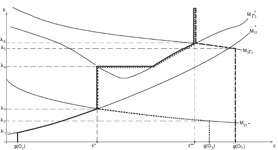
Figure 2: A case of three equilibrium points without changes in the hierarchy of cycles

Let us assume that $\lambda_{1}<\lambda_{2}<\lambda_{3}<\lambda_{4}<\lambda_{5}$ (see Figure 2). For $\lambda<\lambda_{3}$, the behavior of the solution in $D_{1}$ and $D_{2}$ is still governed by Theorem 3.1. For each $\lambda>\lambda_{3}$, the value of $u^{\varepsilon}(T^{\varepsilon}(\lambda),x)$ will be nearly constant on $D_{1}^{\delta}\cup D_{2}^{\delta}$, and we can treat the cycle $\Gamma=\{O_{1},O_{2}\}$ in the same way a single equilibrium was treated in Section 3. Namely, let

$$c^{\Gamma}(\lambda)=\left\{\begin{array}[]{lll}c^{*},~{}~{}~{}~{}~{}~{}~{}~{}~{}~{}~{}~{}~{}~{}~{}~{}~{}~{}~{}~{}~{}~{}~{}~{}~{}~{}~{}~{}~{}~{}~{}~{}~{}~{}~{}~{}~{}~{}~{}~{}~{}~{}~{}~{}~{}~{}~{}~{}~{}~{}~{}~{}~{}~{}~{}~{}~{}~{}~{}~{}~{}~{}~{}\,\lambda_{3}\leq\lambda<\lambda_{4},\\ \min\{g(O_{3}),\min\{c:c\in[c^{*},g(O_{3})],M_{\Gamma 3}(c)=\lambda\}\},~{}~{}\,\,\lambda\geq\lambda_{4},\end{array}\right.$$

$$c^{3}(\lambda)=\left\{\begin{array}[]{lll}g(O_{3}),~{}~{}~{}~{}~{}~{}~{}~{}~{}~{}~{}~{}~{}~{}~{}~{}~{}~{}~{}~{}~{}~{}~{}~{}~{}~{}~{}~{}~{}~{}~{}~{}~{}~{}~{}~{}~{}~{}~{}~{}~{}~{}~{}~{}~{}~{}~{}~{}~{}~{}~{}~{}~{}~{}\,0<\lambda<\lambda_{5},\\ \max\{c^{*},\max\{c:c\in[c^{*},g(O_{3})],M_{3\Gamma}(c)=\lambda\}\},~{}~{}\,\,\lambda\geq\lambda_{5},\end{array}\right.$$

Define $\lambda_{6}=\inf\{\lambda>\lambda_{3}:c^{\Gamma}(\lambda)\geq c^{3}(\lambda)\}$. Assume that $\lambda_{5}<\lambda_{6}$ and that at least one of the functions $c^{\Gamma}$ and $c^{3}$ is continuous at $\lambda_{6}$. Let $c^{**}=c^{\Gamma}(\lambda_{6})$ if $c^{\Gamma}$ is continuous at $\lambda_{6}$ and $c^{**}=c^{3}(\lambda_{6})$ otherwise. Define $\overline{c}^{1}(\lambda)=\overline{c}^{2}(\lambda)=\min(c^{\Gamma}(\lambda),c^{**})$, $\lambda\geq\lambda_{3}$, and $\overline{c}^{3}(\lambda)=\max(c^{3}(\lambda),c^{**})$, $\lambda>0$.

Having thus defined the functions $\overline{c}^{i}(\lambda)$, $i=1,2,3$, for all $\lambda>0$, we can now state that for each $\lambda>0$ such that $\overline{c}^{i}$ is continuous at $\lambda$ and every $\delta>0$, the limit

$$\lim_{\varepsilon\downarrow 0}u^{\varepsilon}(T^{\varepsilon}(\lambda),x)=\overline{c}^{i}(\lambda)$$

is uniform in $x\in D_{i}^{\delta}$.

On Figure 2, the limits $\lim_{\varepsilon\downarrow 0}u^{\varepsilon}(T^{\varepsilon}(\lambda),x)$, as functions of $\lambda$, for $x\in D_{1}^{\delta}$, $D_{2}^{\delta}$ and $D_{3}^{\delta}$ are depicted by thick, dotted and dashed lines, respectively.

5 A general result for the case when the hierarchy of cycles does not change

In this section we will suppose that, in addition to Assumption A, the hierarchy of cycles and the equilibrium points $\nu(\Gamma)$ for each cycle $\Gamma$ of rank less than $R$ do not depend on the choice of constants $c_{i}\in[g_{\rm min},g_{\rm max}]$ in the function $\alpha=a(x,\sum_{i=1}^{n}c_{i}\chi_{D_{i}}(x))$.

We will say that a cycle $\Gamma$ is active for a given value of $\lambda>0$ if $V^{\alpha}_{\Gamma,\nu(\Gamma)}<\lambda$. We will say that it is engaged if $V^{\alpha}_{\Gamma,\nu(\Gamma)}=\lambda$ and passive if $V^{\alpha}_{\Gamma,\nu(\Gamma)}>\lambda$. We will say that a cycle $\Gamma_{0}$ is connected to a cycle $\Gamma$ by a chain if there is a sequence of cycles $\Gamma_{1},...,\Gamma_{k}$ and equilibriums $O_{1}\in\Gamma_{1}$,…,$O_{k}\in\Gamma_{k}$, $O_{k+1}\in\Gamma$ such that $\Gamma_{i}$ are engaged or active and $O_{i+1}=\nu(\Gamma_{i})$ for $0\leq i\leq k$. The collection of all the cycles that do not belong to $\Gamma$ and are connected to $\Gamma$ by a chain will be called the cluster connected to $\Gamma$. For each cycle $\Gamma$ of less than maximal rank and $c\in[g_{\rm min},g_{\rm max}]$, we define

$$M_{\Gamma}(c)=V_{\Gamma,\nu(\Gamma)}^{a(\cdot,c)}$$

and, for $\lambda>0$ and $c_{2}\geq c_{1}$, define $C(c_{1},c_{2},\lambda,\Gamma)=\min(c_{2},\inf(c>c_{1}:M_{\Gamma}(c)\geq\lambda))$. Similarly, if $c_{2}\leq c_{1}$, define $C(c_{1},c_{2},\lambda,\Gamma)=\max(c_{2},\sup(c<c_{1}:M_{\Gamma}(c)\geq\lambda))$.

In Figure 3 we have an example of a hierarchy of cycles with the thick arrows between the actively connected cycles and the corresponding equilibrium points. The dashed arrows are used for the engaged cycles and the dotted arrows for the passively connected cycles.

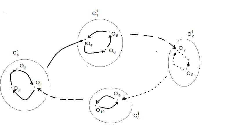
Figure 3: The hierarchy of cycles

In order to describe the asymptotics of $u^{\varepsilon}(T^{\varepsilon}(\lambda),x)$, we will define a finite number of “special” points $0=\lambda_{0}<\lambda_{1}<...<\lambda_{m}=\infty$. We claim that there are functions $\overline{c}^{i}(\lambda)$, $1\leq i\leq n$, which are continuous on each of the intervals $(\lambda_{k},\lambda_{k+1})$, $0\leq k\leq m-1$, have one-sided limits as $\lambda$ approaches the end points of the intervals, and are such that the limits

$$\lim_{\varepsilon\downarrow 0}u^{\varepsilon}(T^{\varepsilon}(\lambda),x)=\overline{c}^{i}(\lambda)$$

are uniform in $x\in D_{i}^{\delta}$ for each $\delta>0$, $\lambda\in\mathbb{R}^{+}\setminus\Lambda$ with $\Lambda=\{\lambda_{0},\lambda_{1},....,\lambda_{m}\}$. Moreover, neither of the cycles changes its type (between passive, engaged and active) for $\lambda\in(\lambda_{k},\lambda_{k+1})$ and $\alpha(x)=\lim_{\varepsilon\downarrow 0}a(x,u^{\varepsilon}(T^{\varepsilon}(\lambda),x))$. We will use induction on $k$ in order to define the functions $\overline{c}^{i}(\lambda)$ and describe for each cycle whether it is passive, engaged or active for $\lambda\in(\lambda_{k},\lambda_{k+1})$ with $\alpha(x)=\lim_{\varepsilon\downarrow 0}a(x,u^{\varepsilon}(T^{\varepsilon}(\lambda),x))$. In the process, we will make several assumptions about the functions $M_{\Gamma}$.

Assuming that we have defined $\overline{c}^{i}(\lambda)$, let

$$\lambda_{\Gamma}=\inf\{\lambda>0:\overline{c}^{i}(\lambda^{\prime})~{}~{}{\rm does}~{}{\rm not}~{}{\rm depend}~{}{\rm on}~{}i~{}{\rm for}~{}\lambda^{\prime}\geq\lambda~{}{\rm and}~{}O_{i}\in\Gamma\}.$$

From the inductive construction of the functions $\overline{c}^{i}(\lambda)$ it will follow that $\lambda_{\Gamma}<\infty$. Let $a_{\Gamma}=\lim_{\lambda\downarrow\lambda_{\Gamma}}\overline{c}^{i}(\lambda)$, $O_{i}\in\Gamma$, and $A_{\Gamma}=M_{\Gamma}(a_{\Gamma})$. We assume that all $A_{\Gamma}$ are distinct and define

$$\Lambda^{1}=\{A_{\Gamma},~{}{\rm rank}(\Gamma)<R\}.$$

We assume that $M_{\Gamma}$ has a finite number of critical points on $[g_{\rm min},g_{\rm max}]$ for each $\Gamma$ with ${\rm rank}(\Gamma)<R$. Let $c^{\Gamma}_{1},...,c^{\Gamma}_{k_{\Gamma}}$ be all the local maxima of $M_{\Gamma}$. We assume that $M_{\Gamma}(c^{\Gamma}_{i})$ are distinct for all $\Gamma$ with ${\rm rank}(\Gamma)<R$ and $i$. Define

$$\Lambda^{2}=\{M_{\Gamma}(c^{\Gamma}_{i}),~{}~{}{\rm rank}(\Gamma)<R,~{}1\leq i\leq k_{\Gamma}\}.$$

Let $\Gamma$ be a cycle of rank $r<R$, $\overline{\Gamma}$ the cycle of rank $r+1$ that contains $\Gamma$, and $\Upsilon$ a cycle that is contained in $\overline{\Gamma}\setminus\Gamma$. Let $I_{\Gamma,\Upsilon}=\{c:M_{\Gamma}(c)=M_{\Upsilon}(c)\}$. We assume that the sets $I_{\Gamma,\Upsilon}$ are finite and $I_{\Gamma_{1},\Upsilon_{1}}\cap I_{\Gamma_{2},\Upsilon_{2}}=\emptyset$ unless $(\Gamma_{1},\Upsilon_{1})=(\Gamma_{2},\Upsilon_{2})$ or $(\Gamma_{1},\Upsilon_{1})=(\Upsilon_{2},\Gamma_{2})$. Define

$$\Lambda^{3}=\{M_{\Gamma}(c),~{}c\in I_{\Gamma,\Upsilon},~{}~{}{\rm rank}(\Gamma)<R,\Upsilon\subseteq\overline{\Gamma}\setminus\Gamma\}.$$

We assume that the numbers $M_{\Gamma}(a_{\Upsilon})$ are distinct for all choices of cycles $\Gamma$ and $\Upsilon$ such that ${\rm rank}(\Gamma)<R$, ${\rm rank}(\Upsilon)\leq{\rm rank}({\Gamma})$ and $\nu(\Gamma)\in\Upsilon$. Define

$$\Lambda^{4}=\{M_{\Gamma}(a_{\Upsilon}),~{}~{}{\rm rank}(\Gamma)<R,~{}{\rm rank}(\Upsilon)\leq{\rm rank}({\Gamma}),~{}\nu(\Gamma)\in\Upsilon\}.$$

Finally, we assume that the sets $\Lambda^{1}$, $\Lambda^{2}$, $\Lambda^{3}$ and $\Lambda^{4}$ do not intersect and define

$$\Lambda=\{\lambda_{0},\lambda_{1},....,\lambda_{m}\}:=\{0\}\cup\Lambda^{1}\cup\Lambda^{2}\cup\Lambda^{3}\cup\Lambda^{4}\cup\{\infty\},$$

where we arrange $\lambda_{k}$ in the increasing order.

Below we will define $\overline{c}^{i}(\lambda)$ on the successive intervals $(\lambda_{k},\lambda_{k+1})$ using induction on $k$ while assuming that $\lambda_{k}$ are known. The above definition of $\Lambda^{1}$ and $\Lambda^{4}$ in terms of $\overline{c}^{i}(\lambda)$ does not constitute a circular argument, since we could instead define the pairs $(\lambda_{k+1},\overline{c}^{i}(\lambda)~{}{\rm for}~{}\lambda\in(\lambda_{k},\lambda_{k+1}))$ inductively. Such an approach would lead to more complicated notations, though, so we avoid it.

Let us proceed with the inductive definition of $\overline{c}^{i}(\lambda)$. For $\lambda\in(\lambda_{0},\lambda_{1})$ all cycles are passive and $\overline{c}^{i}(\lambda)=g(O_{i})$ for all $i$. Assuming that the types of the cycles and the limits $q(O_{i})=\lim_{\lambda\uparrow\lambda_{k}}\overline{c}^{i}(\lambda)$ are known for $\lambda\in(\lambda_{k-1},\lambda_{k})$ with some $0<k<m$, we will describe the types of the cycles for $\lambda\in(\lambda_{k},\lambda_{k+1})$ and specify the limits $s(O_{i})=\lim_{\lambda\downarrow\lambda_{k}}\overline{c}^{i}(\lambda)$. Then, assuming that the types of the cycles are specified for $\lambda\in(\lambda_{k},\lambda_{k+1})$ and the values of $s(O_{i})$ are known, we will define the functions $\overline{c}^{i}(\lambda)$ for $\lambda\in(\lambda_{k},\lambda_{k+1})$. We distinguish a number of cases depending on whether $\lambda_{k}$ belongs to $\Lambda^{1}$, $\Lambda^{2}$, $\Lambda^{3}$ or $\Lambda^{4}$.

First, however, we describe the procedure for determining the values of $s(O_{i})$ for $O_{i}$ which belong to a cluster.

Determining the values of $s(O_{i})$ and the types of cycles within a cluster. Suppose that we have defined $s(O_{i})=\lim_{\lambda\downarrow\lambda_{k}}\overline{c}^{i}(\lambda)$ for all $O_{i}$ that belong to a cycle $\Gamma$. Consider the cluster of cycles that are connected to $\Gamma$ for $\lambda\in(\lambda_{k-1},\lambda_{k})$. For each cycle $\Gamma^{\prime}$ in the cluster, we will define the values of $s(O)$ for $O\in\Gamma^{\prime}$ and specify its type for $\lambda\in(\lambda_{k},\lambda_{k+1})$.

First assume that $\nu(\Gamma^{\prime})=O_{i}\in\Gamma$ for $\lambda\in(\lambda_{k-1},\lambda_{k})$. It will follow from the inductive construction that $q({O^{\prime}})=q(O^{\prime\prime})$ if $O^{\prime},O^{\prime\prime}\in\Gamma^{\prime}$. Let $q(\Gamma^{\prime})=q({O^{\prime}})$. For $O\in\Gamma^{\prime}$, we define $s(O)=C(q(\Gamma^{\prime}),s(O_{i}),\lambda_{k},\Gamma^{\prime})$.

For any cycle $\Gamma^{\prime\prime}$ such that $\nu(\Gamma^{\prime\prime})\in\Gamma^{\prime}$, we can similarly determine the values of $s(O)$ for $O\in\Gamma^{\prime\prime}$. Continuing this procedure inductively, we define the values of $s(O)$ when $O$ belongs to either of the cycles from the cluster. A cycle $\Gamma^{\prime}$ from the cluster will be engaged for $\lambda\in(\lambda_{k},\lambda_{k+1})$ if $\lambda_{k}=M_{\Gamma^{\prime}}(s(O))$ for $O\in\Gamma^{\prime}$ and active if $\lambda_{k}>M_{\Gamma^{\prime}}(s(O))$ for $O\in\Gamma^{\prime}$.

Case 1. Assume that $\lambda_{k}\in\Lambda_{1}$. Let $\Gamma$ be such that $\lambda_{k}=A_{\Gamma}$. For $O_{i}\in\Gamma$, we define $s(O_{i})=C(q(O_{i}),q(\nu(\Gamma)),\lambda_{k},\Gamma)$. The cycle will be engaged for $\lambda\in(\lambda_{k},\lambda_{k+1})$ if $\lambda_{k}=M_{\Gamma}(s(O))$ for $O\in\Gamma$ and active if $\lambda_{k}>M_{\Gamma}(s(O))$ for $O\in\Gamma$.

The types of cycles that belong the the cluster connected to $\Gamma$ for $\lambda\in(\lambda_{k-1},\lambda_{k})$, and the values of $s(O_{j})$ for the equilibrium points in those cycles are determined according to the procedure described above. For the remaining equilibrium points $O$, we define $s(O)=q(O)$. The remaining cycles don’t change type.

Case 2. Assume that $\lambda_{k}\in\Lambda_{2}$. Let $c$ be the local maximum of a cycle $\Gamma$ such that $M_{\Gamma}(c)=\lambda_{k}$. If $\Gamma$ was not engaged for $\lambda\in(\lambda_{k-1},\lambda_{k})$ or if $q(O)\neq c$ for some $O\in\Gamma$, then we define $s(O)=q(O)$ for all the equilibrium points, and all the cycles have the same type on $(\lambda_{k},\lambda_{k+1})$ as on $(\lambda_{k-1},\lambda_{k})$.

If $\Gamma$ was engaged and $q(O)=c$ for $O\in\Gamma$, then for $O_{i}\in\Gamma$, we define $s(O_{i})=C(q(O_{i}),q(\nu(\Gamma)),\lambda_{k},\Gamma)$. The cycle will be engaged for $\lambda\in(\lambda_{k},\lambda_{k+1})$ if $\lambda_{k}=M_{\Gamma}(s(O))$ for $O\in\Gamma$ and active if $\lambda_{k}>M_{\Gamma}(s(O))$ for $O\in\Gamma$.

The types of cycles that belong the the cluster connected to $\Gamma$ for $\lambda\in(\lambda_{k-1},\lambda_{k})$, and the values of $s(O_{j})$ for the equilibrium points in those cycles are determined according to the procedure described above. For the remaining equilibrium points $O$, we define $s(O)=q(O)$. The remaining cycles don’t change type.

Case 3. Assume that $\lambda_{k}\in\Lambda_{3}$. Let $\Gamma$ be a cycle of rank $r<R$, $\overline{\Gamma}$ the cycle of rank $r+1$ that contains $\Gamma$, and $\Upsilon$ a cycle that is contained in $\overline{\Gamma}\setminus\Gamma$. Suppose that $c$ is such that $M_{\Gamma}(c)=M_{\Upsilon}(c)$ and $\lambda_{k}=M_{\Gamma}(c)$.

We define $s(O)=q(O)$ for all the equilibrium points. All the cycles, other than perhaps $\Gamma$ and $\Upsilon$, have the same type on $(\lambda_{k},\lambda_{k+1})$ as on $(\lambda_{k-1},\lambda_{k})$. To determine the type of cycles $\Gamma$ and $\Upsilon$ on $(\lambda_{k},\lambda_{k+1})$, we examine several cases.

(a) If $q(O)=c$ for all $O\in\Gamma\cup\Upsilon$, $\Gamma$ and $\Upsilon$ were engaged, $\Upsilon$ was connected to $\Gamma$ by a chain that contained only active cycles (other than $\Upsilon$ itself) and $\Gamma$ was connected to $\Upsilon$ by a chain that contained only active cycles (other than $\Gamma$ itself), then $\Gamma$ and $\Upsilon$ becomes active.

(b) If $q(O)=c$ for all $O\in\Gamma\cup\Upsilon$, $\Gamma$ was connected to $\Upsilon$ by a chain that contained only active cycles (other than $\Gamma$ itself), but $\Upsilon$ was not connected to $\Gamma$ by a chain that contained only active cycles (other than $\Upsilon$ itself), and $\Upsilon$ was not passive, then $\Gamma$ becomes active on $(\lambda_{k},\lambda_{k+1})$ if it was engaged on $(\lambda_{k-1},\lambda_{k})$ and becomes engaged if it was active. The type of $\Upsilon$ stays the same.

(c) the same as (b) with $\Gamma$ and $\Upsilon$ interchanged.

(d) If none of the cases (a)-(c) applies, then $\Gamma$ and $\Upsilon$ have the same types on $(\lambda_{k},\lambda_{k+1})$ as on $(\lambda_{k-1},\lambda_{k})$.

Case 4. Assume that $\lambda_{k}\in\Lambda_{4}$. Let $\lambda_{k}=M_{\Gamma}(a_{\Upsilon})$, where cycles $\Gamma$ and $\Upsilon$ are such that ${\rm rank}(\Gamma)<R$, ${\rm rank}(\Upsilon)\leq{\rm rank}({\Gamma})$ and $\nu(\Gamma)\in\Upsilon$. We define $s(O)=q(O)$ for all the equilibrium points. All the cycles, other than perhaps $\Gamma$, have the same type on $(\lambda_{k},\lambda_{k+1})$ as on $(\lambda_{k-1},\lambda_{k})$.

The cycle $\Gamma$ becomes active if it was engaged on $(\lambda_{k-1},\lambda_{k})$, $q(O)=a_{\Upsilon}$ for all $O\in\Gamma$ and $M_{\Gamma}(a_{\Upsilon})<A_{\Upsilon}$. Otherwise, $\Gamma$ has the same type on $(\lambda_{k},\lambda_{k+1})$ as on $(\lambda_{k-1},\lambda_{k})$.

Now let us define the functions $\overline{c}^{i}(\lambda)$ on $(\lambda_{k},\lambda_{k+1})$ assuming that the values of $s(O_{i})$ and the cycle types are known. For an equilibrium point $O_{i}$, we identify the cycle $\Gamma$ with the smallest possible rank $r$ such that $O_{i}\in\Gamma$ and the values of $s(O_{j})$, $O_{j}\in\Gamma$, are not all the same. If no such cycle exists, that is if $s(O_{j})$, $1\leq j\leq n$, does not depend on $j$, then we define $\overline{c}^{i}(\lambda)=s(O_{i})$ for $\lambda>\lambda_{k}$.

Assuming that such a cycle $\Gamma$ exists, let $\Gamma_{1},...,\Gamma_{l}$ be the cycles of rank $r-1$ which comprise $\Gamma$, and let $O\in\Gamma_{1}$. Here we number the cycles in such a way that $\mathcal{N}(\Gamma_{1})=\Gamma_{2}$,…,$\mathcal{N}(\Gamma_{l})=\Gamma_{1}$. Take the least $j$ such that $\Gamma_{j}$ is either passive or engaged (it can not happen that all the cycles $\Gamma_{1},...,\Gamma_{l}$ are active, since then all the values of $s(O)$, $O\in\Gamma$, would be the same, as follows from the inductive construction above). If $\Gamma_{j}$ is passive, we define $\overline{c}^{i}(\lambda)=s(O_{i})$ for $\lambda\in(\lambda_{k},\lambda_{k+1})$. If $\Gamma_{j}$ is engaged, we define $\overline{c}^{i}(\lambda)=C(r(O_{i}),\zeta,\lambda,\Gamma_{j})$ for $\lambda\in(\lambda_{k},\lambda_{k+1})$, where $\zeta=+\infty$ if $M_{\Gamma_{j}}$ is locally increasing at $r(O_{i})$ and $\zeta=-\infty$ if $M_{\Gamma_{j}}$ is locally decreasing at $r(O_{i})$.

We can now summarize the above discussion.

Theorem 5.1.

Suppose that Assumption A holds and the hierarchy of cycles and the equilibrium points $\nu(\Gamma)$ for each cycle $\Gamma$ of rank less than $R$ do not depend on the choice of the constants $c_{i}\in[g_{\rm min},g_{\rm max}]$ in the function $\alpha=a(x,\sum_{i=1}^{n}c_{i}\chi_{D_{i}}(x))$. Also suppose that the above assumptions on the sets $\Lambda^{1}$, $\Lambda^{2}$, $\Lambda^{3}$ and $\Lambda^{4}$ hold.

Then the limits

$$\lim_{\varepsilon\downarrow 0}u^{\varepsilon}(T^{\varepsilon}(\lambda),x)=\overline{c}^{i}(\lambda)$$

are uniform in $x\in D_{i}^{\delta}$ for each $\delta>0$, $\lambda\in\mathbb{R}^{+}\setminus\Lambda$, where the functions $\overline{c}^{i}(\lambda)$ were defined via the inductive procedure above.

6 Example of a change in the hierarchy of cycles

As in Section 4, we assume that there are three equilibrium points $O_{1},O_{2},O_{3}$. For each $c_{1},c_{2},c_{3}\in[g_{\rm min},g_{\rm max}]$, the function $f_{c_{1},c_{2},c_{3}}$ is defined by (36). We will assume that the hierarchy of cycles for $\alpha=a(x,f_{c_{1},c_{2},c_{3}}(x))$ depends only on $c_{2}$. This is the case, for example, if $d=1$ and $O_{1}<O_{2}<O_{3}$. More precisely, suppose that there is $\overline{c}\in(g_{\rm min},g_{\rm max})$ such that Assumption A holds for each choice of the constants $c_{i}\in[g_{\rm min},g_{\rm max}]$ such that $c_{2}\neq\overline{c}$. We assume that $O_{1}$ and $O_{2}$ form a cycle $\Gamma^{\prime}=\{O_{1},O_{2}\}$ of rank one when $c_{2}<\overline{c}$, while $O_{2}$ and $O_{3}$ form a cycle $\Gamma^{\prime\prime}=\{O_{2},O_{3}\}$ of rank one when $c_{2}>\overline{c}$.

As before, we will identify a number of “special” points $\lambda_{k}$ and describe the asymptotic behavior of $u^{\varepsilon}(T^{\varepsilon}(\lambda),x)$ for $\lambda\in(\lambda_{k},\lambda_{k+1})$ and $x\in D^{\delta}_{i}$, $i=1,2,3$. In the process, we will make various assumptions about the quasi-potential that will be specific to the example at hand.

In our example we assume that $g(O_{1})\leq g(O_{2})\leq\overline{c}\leq g(O_{3})$. Define

$$M_{12}(c)={V}^{a(\cdot,c)}_{O_{1},O_{2}},~{}M_{21}(c)={V}^{a(\cdot,c)}_{O_{2},O_{1}},~{}M_{\Gamma^{\prime}3}(c)={V}^{a(\cdot,c)}_{\Gamma^{\prime},O_{3}},~{}~{}c\in[g_{\rm min},\overline{c});$$

$$M_{32}(c)={V}^{a(\cdot,c)}_{O_{3},O_{2}},~{}M_{23}(c)={V}^{a(\cdot,c)}_{O_{2},O_{3}},~{}M_{\Gamma^{\prime\prime}1}(c)={V}^{a(\cdot,c)}_{\Gamma^{\prime\prime},O_{1}},~{}M_{1\Gamma^{\prime\prime}}(c)={V}^{a(\cdot,c)}_{O_{1},\nu(O_{1})},~{}~{}c\in(\overline{c},g_{\rm max}].$$

Let $\lambda_{1}=M_{12}(g(O_{1}))$ and $\lambda_{2}=M_{21}(g(O_{2}))$. Define functions $c^{1}$ and $c^{2}$ by (21) and (22), respectively. Let $\lambda_{3}=\inf\{\lambda:c^{1}(\lambda)\geq c^{2}(\lambda)\}$. Assume that at least one of the functions $c^{1}$ and $c^{2}$ is continuous at $\lambda_{3}$. Let $c^{*}=c^{1}(\lambda_{3})$ if $c^{1}$ is continuous at $\lambda_{3}$ and $c^{*}=c^{2}(\lambda_{3})$ otherwise. Let $\overline{c}^{1}(\lambda)=\min(c^{1}(\lambda),c^{*})$ and $\overline{c}^{2}(\lambda)=\max(c^{2}(\lambda),c^{*})$, $\lambda<\lambda_{3}$. Let $\lambda_{4}=M_{\Gamma^{\prime}3}(c^{*})$, $\lambda_{5}=\sup_{c\in[c^{*},\overline{c})}M_{\Gamma^{\prime}3}({c})$ and $\lambda_{6}=M_{32}(g(O_{3}))$.

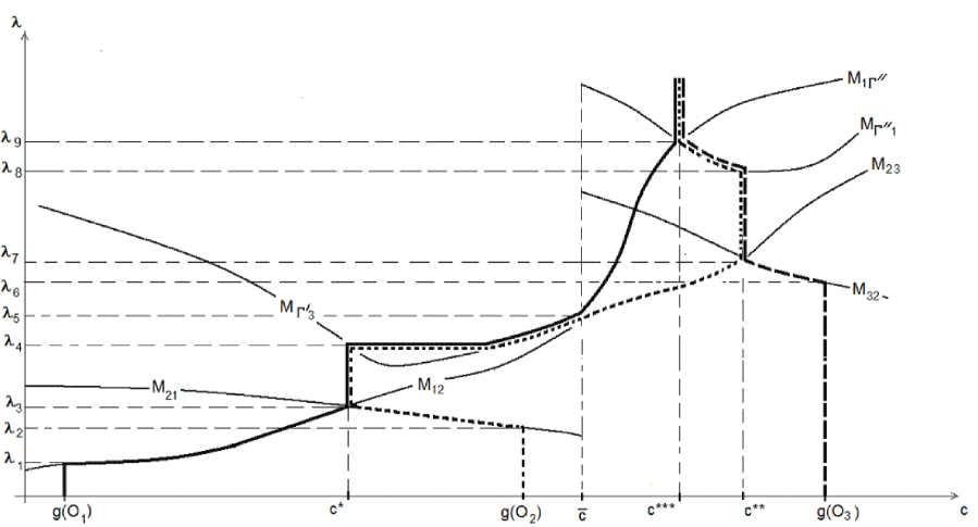
Figure 4: A case of three equilibrium when the hierarchy of cycles changes

Let us assume that $\lambda_{1}<\lambda_{2}<\lambda_{3}<\lambda_{4}<\lambda_{5}<\lambda_{6}$ (see Figure 4). Define

$$\overline{c}^{1}(\lambda)=\overline{c}^{2}(\lambda)=c^{\Gamma^{\prime}}(\lambda)=\left\{\begin{array}[]{lll}c^{*},~{}~{}~{}~{}~{}~{}~{}~{}~{}~{}~{}~{}~{}~{}~{}~{}~{}~{}~{}~{}~{}~{}~{}~{}~{}~{}~{}~{}~{}~{}~{}~{}~{}~{}~{}~{}~{}~{}~{}~{}~{}~{}~{}~{}~{}~{}~{}~{}~{}~{}~{}~{}~{}\,\lambda_{3}\leq\lambda<\lambda_{4},\\ \min\{c:c\in[c^{*},\overline{c}),M_{\Gamma^{\prime}3}(c)=\lambda\},~{}~{}~{}~{}~{}~{}~{}~{}~{}~{}~{}~{}~{}~{}\,\,\lambda_{4}\leq\lambda<\lambda_{5},\end{array}\right.$$

In order to formulate the results on the asymptotics of $u^{\varepsilon}(T^{\varepsilon}(\lambda),x)$ for $\lambda>\lambda_{5}$, we need the functions $d^{2}(\lambda)$ and $c^{3}(\lambda)$ defined as follows:

$$d^{2}(\lambda)=\min\{g(O_{3}),\min\{c:c\in[\overline{c},g(O_{3})],M_{23}(c)=\lambda\}\},~{}~{}\lambda\geq\lambda_{5},$$

$$c^{3}(\lambda)=\left\{\begin{array}[]{lll}g(O_{3}),~{}~{}~{}~{}~{}~{}~{}~{}~{}~{}~{}~{}~{}~{}~{}~{}~{}~{}~{}~{}~{}~{}~{}~{}~{}~{}~{}~{}~{}~{}~{}~{}~{}~{}~{}~{}~{}~{}~{}~{}~{}~{}~{}~{}~{}~{}~{}~{}~{}~{}~{}~{}~{}~{}\,0<\lambda<\lambda_{6},\\ \max\{\overline{c},\max\{c:c\in[\overline{c},g(O_{3})],M_{32}(c)=\lambda\}\},~{}~{}~{}~{}\,\,\lambda\geq\lambda_{6}.\end{array}\right.$$

Let $\lambda_{7}=\inf\{\lambda:d^{2}(\lambda)\geq c^{3}(\lambda)\}$. Assume that $\lambda_{6}<\lambda_{7}$ and at least one of the functions $d^{2}$ and $c^{3}$ is continuous at $\lambda_{7}$. Let $c^{**}=d^{2}(\lambda_{7})$ if $d^{2}$ is continuous at $\lambda_{7}$ and $c^{**}=c^{3}(\lambda_{7})$ otherwise. Let $\lambda_{8}=M_{\Gamma^{\prime\prime}1}(c^{**})$ and assume that $\lambda_{7}<\lambda_{8}$. Define $\overline{c}^{2}(\lambda)=\min(d^{2}(\lambda),c^{**})$, $\lambda_{5}\leq\lambda<\lambda_{8}$, and $\overline{c}^{3}(\lambda)=\max(c^{3}(\lambda),c^{**})$, $0<\lambda<\lambda_{8}$.

Let

$$d^{1}(\lambda)=\min\{c^{**},\min\{c:c\in[\overline{c},c^{**}],M_{1\Gamma^{\prime\prime}}(c)=\lambda\}\},~{}~{}\lambda\geq\lambda_{5},$$

$$c^{\Gamma^{\prime\prime}}(\lambda)=\max\{\overline{c},\max\{c:c\in[\overline{c},c^{**}],M_{\Gamma^{\prime\prime}1}(c)=\lambda\}\},~{}~{}\lambda\geq\lambda_{8}.$$

Let $\lambda_{9}=\inf\{\lambda:d^{1}(\lambda)\geq c^{\Gamma^{\prime\prime}}(\lambda)\}$. Assume that $\lambda_{8}<\lambda_{9}$ and at least one of the functions $d^{1}$ and $c^{\Gamma^{\prime\prime}}$ is continuous at $\lambda_{9}$. Let $c^{***}=d^{1}(\lambda_{9})$ if $d^{1}$ is continuous at $\lambda_{9}$ and $c^{***}=c^{\Gamma^{\prime\prime}}(\lambda_{9})$ otherwise. Define $\overline{c}^{1}(\lambda)=\min(d^{1}(\lambda),c^{***})$, $\lambda_{5}\leq\lambda$ and $\overline{c}^{2}(\lambda)=\overline{c}^{3}(\lambda)=\max(c^{\Gamma^{\prime\prime}}(\lambda),c^{***})$, $\lambda_{8}\leq\lambda$.

Having thus defined the functions $\overline{c}^{i}(\lambda)$, $i=1,2,3$, for all $\lambda>0$, we can now state that for each $\lambda>0$ such that $\overline{c}^{i}$ is continuous at $\lambda$ and every $\delta>0$, the limit

$$\lim_{\varepsilon\downarrow 0}u^{\varepsilon}(T^{\varepsilon}(\lambda),x)=\overline{c}^{i}(\lambda)$$

is uniform in $x\in D_{i}^{\delta}$.

On Figure 4, the limits $\lim_{\varepsilon\downarrow 0}u^{\varepsilon}(T^{\varepsilon}(\lambda),x)$, as functions of $\lambda$, for $x\in D_{1}^{\delta}$, $D_{2}^{\delta}$ and $D_{3}^{\delta}$ are depicted by thick, dotted and dashed lines, respectively.

Acknowledgements: While working on this article, M. Freidlin was supported by NSF grants DMS-0803287 and DMS-0854982 and L. Koralov was supported by NSF grants DMS-0706974 and DMS-0854982.

References

[1] Athreya A., Freidlin M.I., Metastability and
Stochastic Resonance in Nearly-Hamiltonian Systems, Stochastics
and Dynamics, 8, 1, pp 1-21, 2008.
[2] Dueschel J-D., Strook D., Large Deviations, AMS
Chelsea Publishing, 2001.
[3] Freidlin M. I., Metastability and Stochastic
Resonance of Multiscale Systems, Contemporary Mathematics, 2008.
[4] Freidlin M. I., Sublimiting Distributions and
Stabilization of Solutions of Parabolic Equations with a Small
Parameter, Soviet Math. Dokl., 235, 5, pp 1042-1045, 1977.
[5] Freidlin M.I., Functional Integration and
Partial Differential Equations, Princeton University Press, 1985.
[6] Freidlin M. I., Quasi-deterministic
Approximation, Metastability and Stochastic Resonance, Physica D,
137, pp 333-352, 2000.
[7] Freidlin M. I., Koralov L. Nonlinear Stochastic Perturbations of Dynamical Systems and
Quasi-linear Parabolic PDE’s with a Small Parameter, Probability
Theory and Related Fields (2010), 147, pp 273-301. (An updated
version is available on the arXiv.)
[8] Freidlin M. I., Wentzell A. D., On small
perturbations of dynamical systems, Russian Math. Surveys 25
(1970), 1-55.
[9] Freidlin M. I., Wentzell A. D., Random
Perturbations of Dynamical Systems, Springer 1998.
[10] Krylov N.V., Nonlinear Elliptic and Parabolic Equations of the Second Order
(Mathematics and its Applications), Springer 1987.
[11] Ladyzenskaya O.A., Ural’zeva N.N., Linear and
Quasi-Linear Parabolic Equations (Russian), Nauka 1967.
[12] Oliveiri E., Vares M.E. Large Deviations and
Metastability, Cambridge University Press, 2005.