Theory of heterotic SIS Josephson junctions between single- and multi-gap superconductors

Abstract

Using the functional integral method, we construct a theory of heterotic SIS Josephson junctions between single- and two-gap superconductors. The theory predicts the presence of in-phase and out-of-phase collective oscillation modes of superconducting phases. The former corresponds to the Josephson plasma mode whose frequency is drastically reduced for $\pm$ s-wave symmetry, and the latter is a counterpart of Leggett’s mode in Josephson junctions. We also reveal that the critical current and the Fraunhofer pattern strongly depend on the symmetry type of the two-gap superconductor.

The Josephson effect is one of the most drastic phenomena in superconductivity Tinkham2004 . Cooper pairs can tunnel through an insulating barrier in a non-dissipative manner. This particular feature has attracted tremendous attention of not only physicists but also device engineers.

Very recently, multi-gap superconductors have been revisited since the discovery of an iron-based high-$T_{{\rm c}}$ superconductor Kamihara;Hosono:2008 ; Takahashi2008 ; Ren;Zhao:2008 . In contrast to cuprate high-$T_{{\rm c}}$ superconductors, 3-$d$ electrons on the iron atom form multi-bands whose Cooper pairs condense into a multi-gap superconducting state. The angle resolved photoemission spectroscopy has reported that each of multiple disconnected Fermi surfaces is fully gapped Ding2008 and other experiments have also supported the gapful features fullgap . On the contrary, the nuclear magnetic resonance have shown typical gapless features Nakai;Hosono;2008 .

In order to compromise the controversy, the presence of $\pm$ s-wave gaps on the disconnected Fermi surfaces has been proposed Mazin;Du:2008 ; Kuroki;Aoki:2008 ; Nagai;Machida:2008 . The essence of the $\pm$ s-wave symmetry is a sign change between different s-wave order parameters. This is expected to bring about novel behaviors in phase interference effects. In particular, Josephson effects in SIS junction between the single- and the $\pm$ s-wave multi-gap superconductors as schematically illustrated in Fig. 1 drastically reflect the sign change. In this Letter, we focus on such a heterotic SIS junction and clarify peculiar Josephson effects. We have three main results, i.e., the drastic reduction of (i) the Josephson plasma frequency, (ii) the critical current, and (iii) the Fraunhofer pattern visibility. The $\pm$ s-wave symmetry leads to a cancellation between the two Josephson currents which arise from the two tunneling channels in this system.

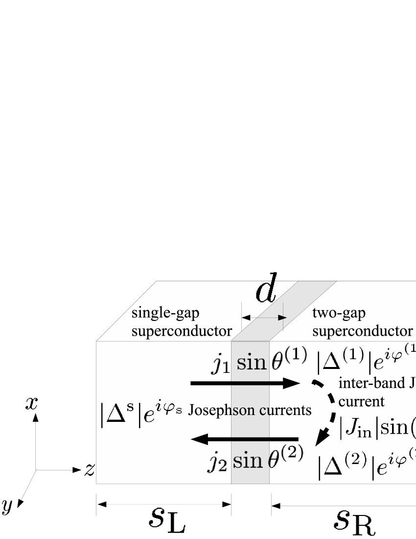
Figure 1: A schematic figure of the present heterotic junction system. The left electrode is a single-gap superconductor, and the right electrode a two-gap superconductor.

In the proposed junction as shown in Fig. 1, the left (right) electrode is a single-(two-)gap superconductor with the width $s_{{\rm L}}$ ($s_{{\rm R}}$). The insulator width and the dielectric constant are $d$ and $\epsilon$, respectively. The current and the magnetic field are applied along $z$- and $y$-direction, respectively. Similar situations were also examined from other viewpoints others .

The system’s Hamiltonian $\hat{H}=\int_{{\rm R}}d^{3}\bm{r}(\mathcal{\hat{H}}^{(1)}_{{\rm R}}+\mathcal{\hat{H}}^{(2)}_{{\rm R}}+\mathcal{\hat{H}}^{{\rm pair}}_{{\rm R}})+\int_{{\rm L}}d^{3}\bm{r}(\mathcal{\hat{H}}^{{\rm s}}_{{\rm L}}+\mathcal{\hat{H}}^{{\rm pair}}_{{\rm L}})+\hat{H}_{{\rm T}}$, where $\mathcal{\hat{H}}^{(i)}_{\rm R}$ describes the kinetic energy of the $i$-th band electrons $\hat{\psi}^{(i)}_{\sigma}$ in the right electrode. The pairing term in the right electrode $\mathcal{\hat{H}}^{{\rm pair}}_{\rm R}=-g_{1}\hat{\psi}^{(1)\,\dagger}_{\uparrow}\hat{\psi}^{(1)\,\dagger}_{\downarrow}\hat{\psi}^{(1)}_{\downarrow}\hat{\psi}^{(1)}_{\uparrow}-g_{2}\hat{\psi}^{(2)\,\dagger}_{\uparrow}\hat{\psi}^{(2)\,\dagger}_{\downarrow}\hat{\psi}^{(2)}_{\downarrow}\hat{\psi}^{(2)}_{\uparrow}-g_{12}(\hat{\psi}^{(1)\,\dagger}_{\uparrow}\hat{\psi}^{(1)\,\dagger}_{\downarrow}\hat{\psi}^{(2)}_{\downarrow}\hat{\psi}^{(2)}_{\uparrow}+\text{h.c.})$ SGB2002 , where $g_{i}>0$, and the inter-band interaction can be either attractive (i.e., $g_{12}>0$) or repulsive (i.e., $g_{12}<0$). The left electrode is described by $\mathcal{\hat{H}}^{{\rm s}}_{{\rm L}}+\mathcal{\hat{H}}^{{\rm pair}}_{{\rm L}}$, where $\mathcal{\hat{H}}^{{\rm s}}_{{\rm L}}$ is the kinetic energy and $\mathcal{\hat{H}}^{{\rm pair}}_{{\rm L}}=-g_{{\rm s}}\hat{\psi}^{{\rm s}\,\dagger}_{\uparrow}\hat{\psi}^{{\rm s}\,\dagger}_{\downarrow}\hat{\psi}^{{\rm s}}_{\downarrow}\hat{\psi}^{{\rm s}}_{\uparrow}$, in which $g_{{\rm s}}>0$. The tunneling Hamiltonian $\hat{H}_{{\rm T}}=\hat{H}_{{\rm T}}^{(1)}+\hat{H}_{{\rm T}}^{(2)}$, where $\hat{H}_{{\rm T}}^{(i)}$ means the tunneling between the electrons in the left side and the $i$-th band electrons in the right side. Using the imaginary time functional integral method Simanek1994 ; MKTT2000 , the effective action with respect to the order parameters $\Delta^{(i)}$ and $\Delta^{{\rm s}}$ is given by $S_{\rm eff}=\int^{\hbar\beta}_{0}\!\!\!d\tau[\!\int_{{\rm R}}d^{3}\bm{r}(g_{2}|\Delta^{(1)}|^{2}/g+g_{1}|\Delta^{(2)}|^{2}/g+V_{\rm in})+\int_{{\rm L}}d^{3}\bm{r}|\Delta^{{\rm s}}|^{2}/g_{{\rm s}}]-{\rm Tr}\ln\hat{G}_{0}-{\rm Tr}\ln\hat{G}^{-1}$, where $\beta$ is the inverse temerature and $V_{{\rm in}}=-g_{12}(\Delta^{(1)\ast}\Delta^{(2)}+\text{c.c.})/g$. We assume here that $g\equiv g_{1}g_{2}-g_{12}^{2}>0$ SGB2002 . The Green functions for the non-interacting system $\hat{G}_{0}$ and the total system $\hat{G}$ are $6\times 6$ matrices. We do not write their explicite expressions here, but those consists of $4\times 4$ for the two-gap and $2\times 2$ for the single-gap superconductors Simanek1994 ; MKTT2000 . The inter-band Josephson coupling term $V_{{\rm in}}$ is rewritten as $V_{{\rm in}}=-2(g_{12}/g)|\Delta^{(1)}|\,|\Delta^{(2)}|\cos(\varphi^{(1)}-\varphi^{(2)})$, in which $\Delta^{(i)}=|\Delta^{(i)}|e^{i\varphi^{(i)}}$.

Based on the standard procedure Simanek1994 ; MKTT2000 , the effective Lagrangian density of the superconducting phases on $zx$-plane in the real time formalisum is given by

$$\mathcal{L}_{{\rm eff}} = \frac{s_{{\rm L}}}{8\pi\mu^{2}}a_{0}^{2}+\sum_{i=1}^{2}\frac{s_{{\rm R}}}{8\pi\mu^{(i)\,2}}a_{0(i)}^{2}-\frac{s_{{\rm L}}}{8\pi\lambda^{2}}a_{x}^{2}$$ (1)

$$-\sum_{i=1}^{2}\frac{s_{{\rm R}}}{8\pi\lambda^{(i)\,2}}a_{x(i)}^{2}-V_{{\rm J}}+\mathcal{L}_{{\rm EM}},$$

where

$$V_{{\rm J}} = -\frac{\hbar j_{1}}{e^{\ast}}\cos\theta^{(1)}-\frac{\hbar j_{2}}{e^{\ast}}\cos\theta^{(2)}-\frac{\hbar J_{{\rm in}}}{e^{\ast}}\cos\varphi,$$ (2)

$$\mathcal{L}_{{\rm EM}} = \frac{\epsilon d}{8\pi}E_{{\rm RL}}^{z\,2}-\frac{d}{8\pi}B_{{\rm RL}}^{y\,2},$$ (3)

$$\theta^{(i)} = \varphi^{(i)}-\varphi_{{\rm s}}-\frac{e^{\ast}d}{\hbar c}A^{z}_{{\rm RL}},$$ (4)

$$\varphi = \varphi^{(1)}-\varphi^{(2)}=\theta^{(1)}-\theta^{(2)},$$ (5)

and note that $a_{0}=(\hbar/e^{\ast})\partial_{t}\varphi_{{\rm s}}+A_{{\rm L}}^{0}$, $a_{x}=(\hbar c/e^{\ast})\partial_{x}\varphi_{{\rm s}}-A_{{\rm L}}^{x}$, $a_{0(i)}=(\hbar/e^{\ast})\partial_{t}\varphi^{(i)}+A_{{\rm R}}^{0}$, $a_{x(i)}=(\hbar c/e^{\ast})\partial_{x}\varphi^{(i)}-A_{{\rm R}}^{x}$, and $e^{\ast}=2e$. The phase $\varphi_{{\rm s}}$ is defined as $\Delta^{{\rm s}}=|\Delta^{{\rm s}}|e^{i\varphi_{{\rm s}}}$, and $j_{i}$ is the Josephson critical current between $i$-th and single-band Cooper pairs. The charge screening length and the penetration depth on the left (right) electrode are $\mu$ ($\mu^{(i)}$) and $\lambda$ ($\lambda^{(i)}$), respectively. The last term in the gauge-invariant phase difference (4) is the $z$ component of the spatial averaged vector potential in the insulator, defined as $A^{z}_{{\rm RL}}=d^{-1}\int_{-d/2}^{d/2}A^{z}(z)\,dz$. The electric and the magnetic fields in the insulator are defined as $E_{{\rm RL}}^{z}=-c^{-1}\partial_{t}A^{z}_{{\rm RL}}-d^{-1}(A^{0}_{{\rm R}}-A^{0}_{{\rm L}})$ and $B_{{\rm RL}}^{y}=d^{-1}(A^{x}_{{\rm R}}-A^{x}_{{\rm L}})-\partial_{x}A^{z}_{{\rm RL}}$, respectively. Here, let us focus on the Josephson coupling energy (2). The first and the second terms are the ordinary Josephson coupling terms, while the third term corresponds to the inter-band Josephson coupling energy and $|J_{{\rm in}}|$ is proportional to $|(g_{12}/g)s_{{\rm R}}|$. One finds that $J_{{\rm in}}$ is positive (negative) if $g_{12}>0$ ($g_{12}<0$). If $s_{{\rm L}}$ and $s_{{\rm R}}$ are much larger than $d$, then it allows us to regard $|J_{{\rm in}}|\gg j_{1},\,j_{2}$.

From Eq. (1), we have the Euler-Lagrange equations with respect to $A^{0}_{l}$ and $A^{x}_{l}$ as follows,

$$\frac{\bar{\alpha}}{\alpha_{1}}\partial_{t}\theta^{(1)}+\frac{\bar{\alpha}}{\alpha_{2}}\partial_{t}\theta^{(2)} = C\frac{e^{\ast}d}{\hbar}E^{z}_{{\rm RL}},$$ (6)

$$\frac{\bar{\eta}}{\eta_{1}}\partial_{x}\theta^{(1)}+\frac{\bar{\eta}}{\eta_{2}}\partial_{x}\theta^{(2)} = L\frac{e^{\ast}d}{\hbar c}B^{y}_{{\rm RL}},$$ (7)

where the dimensionless parameters in each electrode are defined as $\alpha=\epsilon\mu^{2}/s_{{\rm L}}d$, $\alpha_{i}=\epsilon\mu_{i}^{2}/s_{{\rm R}}d$, $\bar{\alpha}^{-1}=\alpha_{1}^{-1}+\alpha_{2}^{-1}$, $\eta=\lambda^{2}/s_{{\rm L}}d$, $\eta_{i}=\lambda^{(i)\,2}/s_{{\rm R}}d$, and $\bar{\eta}^{-1}=\eta_{1}^{-1}+\eta_{2}^{-1}$. The magnitude of the electric (magnetic) field coupling is characterized by $\alpha$ and $\alpha_{i}$ ($\eta$ and $\eta_{i}$) MS2004 . The constants $C$ and $L$ are defined as $C=1+\alpha+\bar{\alpha}$ and $L=1+\eta+\bar{\eta}$, respectively. Equations (6) and (7) correspond to the generalized Josephson relations MKT1999 . The Euler-Lagrange equation with respect to $A^{z}_{{\rm RL}}$ gives the Maxwell equation,

$$\frac{e^{\ast}d}{\hbar c}\partial_{x}B^{y}_{{\rm RL}} = \sum_{i=1}^{2}\frac{1}{\lambda_{{{\rm J}}i}^{2}}\sin\theta^{(i)}+\frac{\epsilon}{c^{2}}\frac{e^{\ast}d}{\hbar}\partial_{t}E^{z}_{{\rm RL}},$$ (8)

where $\lambda_{{{\rm J}}i}^{-2}=4\pi e^{\ast}dj_{i}/\hbar c^{2}$. The first term on the right hand side of Eq. (8) is the summation of the Josephson current terms [Fig. 1]. Using Eqs. (6)-(8), we obtain

$$\sum_{i=1}^{2}\frac{C\bar{\eta}}{\eta_{i}}\partial_{x}^{2}\theta^{(i)}=\sum_{i=1}^{2}\frac{CL}{\lambda_{{\rm J}i}^{2}}\sin\theta^{(i)}+\sum_{i=1}^{2}\frac{L\bar{\alpha}}{\alpha_{i}}\partial_{t}^{2}\theta^{(i)}.$$ (9)

Next, from the Euler-Lagrange equations about $\varphi_{{\rm s}}$ and $\varphi^{(i)}$, we have

$$\frac{\epsilon}{c^{2}}\sum_{i=1}^{2}\bigg{[}(-1)^{i+1}\frac{CL}{\alpha_{i}}\partial_{t}^{2}\theta^{(i)}+\frac{(1+\alpha)\xi L}{\alpha_{i}}\partial_{t}^{2}\theta^{(i)}\bigg{]}$$ (10)

$$= \sum_{i=1}^{2}\bigg{[}(-1)^{i+1}\frac{CL}{\eta_{i}}\partial_{x}^{2}\theta^{(i)}+\frac{(1+\eta)\zeta C}{\eta_{i}}\partial_{x}^{2}\theta^{(i)}\bigg{]}$$

$$-2CL\frac{4\pi e^{\ast}d}{\hbar c^{2}}\frac{\partial V_{{\rm J}}}{\partial\varphi},$$

where the parameter $\xi$ ($\zeta$) means the difference of the magnitude of the electric (magnetic) field coupling between the different superconducting bands as $\xi=(\alpha_{1}-\alpha_{2})/(\alpha_{1}+\alpha_{2})$ and $\zeta=(\eta_{1}-\eta_{2})/(\eta_{1}+\eta_{2})$.

The present description is valid from very thin electrode junctions ($s_{{\rm L}}\sim\mu$ and $s_{{\rm R}}\sim\mu^{(i)}$) to conventional thick ones. In the latter case ($s_{{\rm L}}\gg\mu$ and $s_{{\rm R}}\gg\mu^{(i)}$), we can take an approximate treatment, $\alpha\to 0$ and $\alpha_{i}\to 0$. Remark that the present paper highlight, i.e., particular features due to $\pm$ s-wave is unchanged in this limit.

Now, let us examine the collective modes involved in Eqs.(9) and (10). For this purpose, we linearize them around a stable point of $V$. First, we focus on $J_{{\rm in}}>0$. Then, a stable point for $(\theta^{(1)},\theta^{(2)})$ is $(0,0)$ and the dispersion relations $\omega_{\pm}^{2}(k_{x})$ is given by

$$\omega_{{\pm}}^{2}(J_{{\rm in}}>0)=\frac{X(\omega_{{\rm P}}^{2}+\omega_{{\rm L}}^{2})-2\bar{\alpha}\xi C^{-1}D\pm\sqrt{R}}{2(1-\xi^{2})},$$ (11)

where

$$\left\{\begin{array}[]{l}\omega_{{\rm P}}^{2}=C(\omega_{{\rm p}1}^{2}+\omega_{{\rm p}2}^{2})[1+L^{-1}(k_{x}/K)^{2}],\\ \omega_{{\rm L}}^{2}=\bar{\alpha}X^{-1}\{4\nu_{{\rm in}}^{2}+(\omega_{{\rm p}1}^{2}+\omega_{{\rm p}2}^{2})[1+\bar{\eta}^{-1}Y(k_{x}/K)^{2}]\}.\end{array}\right.$$

The Josephson plasma frequency associated with the Josephson current for $\theta^{(i)}$, $\omega_{{\rm p}i}=c/\sqrt{\epsilon}\lambda_{{{\rm J}}i}$, while the pseudo Josephson-plasma frequency associated with the inter-band Josephson current, $\nu_{{\rm in}}=\sqrt{4\pi e^{\ast}d|J_{\rm in}|/\epsilon\hbar}$. Note that $K^{2}=c^{-2}\epsilon(\omega_{{\rm p}1}^{2}+\omega_{{\rm p}2}^{2})$, the dimensionless parameters $X$ and $Y$ are defined as $X=1-\xi^{2}C^{-1}(1+\alpha)$ and $Y=1-\zeta^{2}L^{-1}(1+\eta)$, respectively, and the quantities $D$ and $R$ are, respectively, $D=C(\omega_{{\rm p}1}^{2}+\omega_{{\rm p}2}^{2})[-\delta+\zeta L^{-1}(k_{x}/K)^{2}]$ and $R=X\{(1-\xi^{2})(\omega_{{\rm P}}^{2}-\omega_{{\rm L}}^{2})^{2}+4\bar{\alpha}C^{-1}[D-\xi(\omega_{{\rm P}}^{2}+\omega_{{\rm L}}^{2})/2]^{2}\}$, where $\delta=(j_{1}-j_{2})/(j_{1}+j_{2})$. When $\xi=\zeta=\delta=0$ (i.e., the superconducting characters are perfectly equivalent between the two bands), we find that $\omega_{+}=\omega_{{\rm P}}$ and $\omega_{-}=\omega_{{\rm L}}$. We then notice that no term related to the inter-band Josephson coupling is involved in the expression of $\omega_{{\rm P}}$. It indicates that the origin of $\omega_{{\rm P}}$ is irrelevant to the motion of the relative phase $\varphi$. Then $\omega_{+}$ corresponds to the in-phase motion for $\theta^{(1)}$ and $\theta^{(2)}$. On the other hand, the origin of $\omega_{-}$ is the out-of-phase motion for $\theta^{(1)}$ and $\theta^{(2)}$. Next, we study another case of $J_{{\rm in}}<0$, in which $(\pi,0)$ is a stable point since $|J_{{\rm in}}|\gg j_{1},j_{2}$. Expanding $V$ around $(\pi,0)$, we have

$$\omega_{\pm}^{2}(J_{\rm in}<0)=\frac{X(\omega_{{\rm P}}^{\prime\,2}+\omega_{{\rm L}}^{\prime\,2})-2\bar{\alpha}\xi C^{-1}D^{\prime}\pm\sqrt{R^{\prime}}}{2(1-\xi^{2})},$$ (12)

where

$$\left\{\begin{array}[]{l}\omega^{\prime\,2}_{{\rm P}}=C(\omega_{{\rm p}1}^{2}+\omega_{{\rm p}2}^{2})(|\delta|+L^{-1}(k_{x}/K)^{2}),\\ \omega^{\prime\,2}_{{\rm L}}=\bar{\alpha}X^{-1}[4\nu_{{\rm in}}^{2}+(\omega_{{\rm p}1}^{2}+\omega_{{\rm p}2}^{2})(|\delta|+\bar{\eta}^{-1}Y(k_{x}/K)^{2}].\end{array}\right.$$

The quantities $D^{\prime}$ and $R^{\prime}$ are $D^{\prime}=C(\omega_{{\rm p}1}^{2}+\omega_{{\rm p}2}^{2})(1+\zeta L^{-1}(k_{x}/K)^{2})$ and $R^{\prime}=X\{(1-\xi^{2})(\omega_{{\rm P}}^{\prime\,2}-\omega_{{\rm L}}^{\prime\,2})^{2}+4\bar{\alpha}C^{-1}[D^{\prime}-\xi(\omega_{{\rm P}}^{\prime\,2}-\omega_{{\rm L}}^{\prime\,2})/2]^{2}\}$, respectively. Figures 2(a) and (b) show the typical dispersion relations for $J_{{\rm in}}>0$ and $J_{{\rm in}}<0$, respectively. For both cases, the frequency of the out-of-phase mode $\omega_{-}$ is found to be lower than the in-phase mode $\omega_{+}$ for an arbitrary value of $k$. Here, we take the limit $k_{x}\to 0$ in Eqs. (11) and (12) to explicitly evaluate the gap frequency for these modes. As for $J_{{\rm in}}>0$, the leading order terms are, respectively, given as $\omega_{+}\simeq(\omega_{{\rm p}1}^{2}+\omega_{{\rm p}2}^{2})^{1/2}$ and $\omega_{-}\simeq(\alpha_{1}+\alpha_{2})^{1/2}\nu_{{\rm in}}$ by regarding $\bar{\alpha}$ and $\alpha$ to be small. However, remark that we keep the term $\bar{\alpha}\nu_{{\rm in}}^{2}(\omega_{{\rm p}1}^{2}+\omega_{{\rm p}2}^{2})^{-1}$ in the above evaluation, because $|J_{{\rm in}}|>j_{1},\,j_{2}$ even though $\bar{\alpha}$ is small. Similarly, when $J_{{\rm in}}<0$, we have $\omega_{+}\simeq|\omega_{{\rm p}1}^{2}-\omega_{{\rm p}2}^{2}|^{1/2}$ and $\omega_{-}\simeq(\alpha_{1}+\alpha_{2})^{1/2}\nu_{{\rm in}}$.

(a)​​ (b)​​

Figure 2: The dispersion relations for $\omega_{\pm}$. The solid (dotted) line is for $\omega_{+}$ ($\omega_{-}$). The parameters are set as follows: $\alpha=\alpha_{1}=10^{-3}$, $\alpha_{2}/\alpha_{1}=1.4$, $\eta=\eta_{1}=10^{3}$, $\eta_{2}/\eta_{1}=1.4$, $j_{2}/j_{1}=0.9$ and $|J_{{\rm in}}|/j_{1}=40.0$. The reduction of $\omega_{+}$ is observed for $J_{{\rm in}}<0$. (a) $J_{{\rm in}}>0$. (b) $J_{{\rm in}}<0$.

The gap of $\omega_{+}$ is characterized by a superposition ($J_{{\rm in}}>0$) or subtraction ($J_{{\rm in}}<0$) between $\omega_{{\rm p}1}$ and $\omega_{{\rm p}2}$. Thus, we refer $\omega_{+}$ to the Josephson plasma mode. We emphasize that the a signature of $\pm$ s-wave is the reduction of plasma frequency [Fig. 2]. On the other hand, since the gap of $\omega_{-}$ is characterized by $\nu_{{\rm in}}$ and $\alpha_{i}$, we find that it corresponds to the gap of the Leggett’s mode, which was derived as a collective mode generated by the density fluctuation between two superfluidities Leggett1966 . Thus, it should be called Josephson-Leggett mode. The inter-band Josephson coupling and the charge density fluctuation create the the mode. Conventionally, the first and the second terms in Eq. (1) are fixed to be zero ($\alpha_{i}\to 0$) because the charge screening length is much smaller than the electrode size. Then, the effective Lagrangian density gives the standard Josephson relation $\partial_{t}\theta^{(i)}=(e^{\ast}d/\hbar)E^{z}_{{\rm RL}}$, resulting in $\partial_{t}(\theta^{(1)}-\theta^{(2)})=0$. It means that the Josephson-Leggett mode becomes a gapless mode. In contrast, the mode $\omega_{{\rm P}}$ can still remain massive in $\alpha_{i}\to 0$. The retainment of non-zero $\alpha_{i}$ is responsible for the finite gap frequency of the Josephson-Leggett mode. The bulk Leggett’s mode is normally embedded in the quasi-particle excitation continuum Blumberg;Karpinski:2007 , while the Josephson-Leggett mode is more clearly and easily observable because the mode lies far beneath the gap energy.

(a)​​  (b)​​  (c)

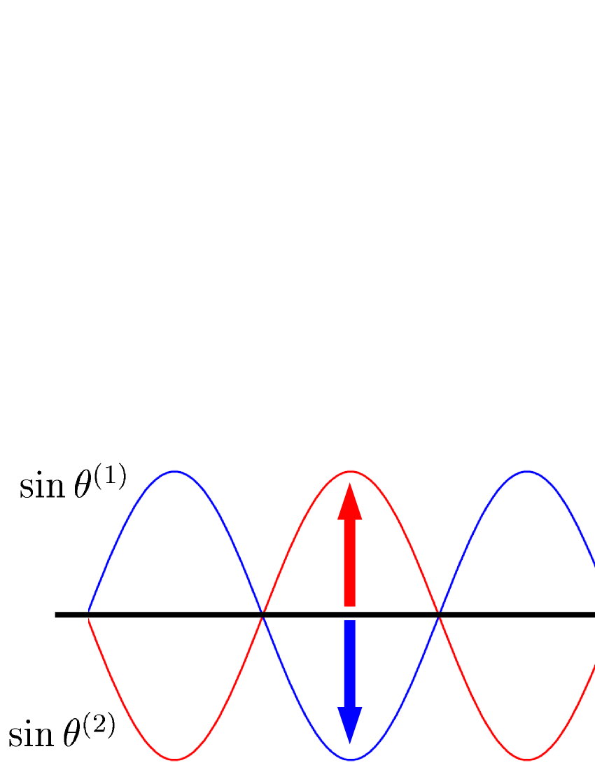
Figure 3: The current vs. the magnetic flux. The value of $I_{0}$ is $I(H^{y}=0)$ for $\varphi=0$. (a) $J_{{\rm in}}>0$ and $\varphi=0$. (b) $J_{{\rm in}}<0$ and $\varphi=\pi$. No current is observed when $j_{1}=j_{2}$. (c) The demonstration of the cancellation between two Josephson currents.

The remaining part of this Letter is devoted to basic Josephson effects. First, let us discuss the Josephson critical current $j_{{\rm c}}$. The bias current is assumed to be uniformly applied without the external magnetic field. Namely, $\theta^{(1)}$ and $\theta^{(2)}$ are assumed to be unifrom along the $x$-axis in Fig. 1. The bias current $I$ is added to the right hand side of Eq. (9) with the elimination of the spatial dependent terms, and $j_{{\rm c}}$ can be derived by estimating the maximum threshold of $I$ under keeping a stationary solution. The condition is given by

$$I = j_{1}\sin\theta^{(1)}+j_{2}\sin\theta^{(2)},$$ (13)

$$0 = -j_{1}\sin\theta^{(1)}+j_{2}\sin\theta^{(2)}-J_{{\rm in}}\sin\varphi.$$ (14)

Equation (13) means that $I$ coincides with the sum of two Josephson currents between the electrodes, while Eq. (14) is an internal current conservation law, which gives a significant constraint on the critical current. When $J_{{\rm in}}>0$, the preferable choice of $\varphi$ is $0$. Equation (14) implies $(j_{1}-j_{2})\sin\theta^{(1)}=0$, because $\theta^{(1)}=\theta^{(2)}$. This is always satisfied if $j_{1}=j_{2}$. Then, since $\theta^{(1)}$ can vary from $0$ to $2\pi$, $j_{{\rm c}}=j_{1}+j_{2}$. If $j_{1}\neq j_{2}$, then $\varphi$ can deviate from $0$ and $j_{{\rm c}}\leq j_{1}+j_{2}$. On the other hand, when $J_{{\rm in}}<0$, $\varphi$ should be $\pi$. Equation (14) implies $(j_{1}+j_{2})\sin\theta^{(1)}=0$. The only possible solution is $\theta^{(1)}=0$ and $\theta^{(2)}=-\pi$, because $j_{1}+j_{2}\neq 0$. Thus, we find that the value of $j_{{\rm c}}$ is drastically reduced compared to the case of $J_{{\rm in}}>0$, e.g., $j_{{\rm c}}=0$ for the case of perfectly identical $\pm$ s-wave two-gap superconductivity.

Next, we consider the Josephson effects in the presence of the external magnetic field $H^{y}$. We focus on stationary solutions, i.e., we drop the temporal terms of $\theta^{(i)}$. According to Eq. (7), $\theta^{(1)}(x)=kx+\theta_{0}+(\bar{\eta}/\eta_{2})\varphi(x)$ and $\theta^{(2)}(x)=kx+\theta_{0}-(\bar{\eta}/\eta_{1})\varphi(x)$, where $k=L(e^{\ast}d/\hbar c)H^{y}$ and $\theta_{0}\in[0,2\pi)$ is an integral constant. The observed current is then given by $I(H^{y},\theta_{0})=\int_{-L_{x}/2}^{L_{x}/2}\left[j_{1}\sin\theta^{(1)}(x)+j_{2}\sin\theta^{(2)}(x)\right]dx$. Hereafter, we assume that $\varphi(x)$ is spatially uniform. Taking account of $|J_{{\rm in}}|>j_{1},\,j_{2}$, we should have $0\approx-J_{{\rm in}}\sin\varphi$ from Eq. (10). When $J_{{\rm in}}>0$ (i.e., $\varphi=0$), the magnetic field dependece of the current is given by $I(H^{y},\theta_{0})=L_{x}\sin\theta_{0}[(j_{1}+j_{2})(\Phi_{0}/\pi\Phi)\sin(\pi\Phi/\Phi_{0})]$, where $\Phi_{0}=2\pi\hbar c/e^{\ast}$ and $\Phi=LH^{y}dL_{x}$. Then, $I(H^{y})\equiv\max_{\theta_{0}}|I(H^{y},\theta_{0})|=L_{x}(j_{1}+j_{2})|(\Phi_{0}/\pi\Phi)\sin(\pi\Phi/\Phi_{0})|$. As a result, we obtain the ordinary Fraunhofer diffraction pattern as a function of the magnetic flux $\Phi$ [Fig. 3(a)]. The maximun value of $I(H^{y})$ is the sum of two Josephson currents as $I(0)=L_{x}(j_{1}+j_{2})$. We also observe that the net current conventionally vanishes when $\Phi=\kappa\Phi_{0}$ ($\kappa\in\mathbb{N}$). In contrast, as for $J_{{\rm in}}<0$ (i.e., $\pm$ s-wave), the current is given by $I(H^{y})=L_{x}|j_{1}-j_{2}||(\Phi_{0}/\pi\Phi)\sin(\pi\Phi/\Phi_{0})|$. If $j_{1}=j_{2}$, the Fraunhofer diffraction pattern completely disappears. When $j_{1}\neq j_{2}$, the pattern is observable except for $\Phi=\kappa\Phi_{0}$, but the maximum value becomes unexpectedly small [Fig. 3(b)]. The situation at $j_{1}=j_{2}$ is schematically displayed in Fig. 3(c). The Josephson currents for $\theta^{(1)}$ and $\theta^{(2)}$ cancel out each other.

Finally, let us discuss how to experimentally confirm the theoretical predictions. We point out that the maximum Josephson current can be estimated from the normal state resistance based on Ambegaokar-Baratoff relation Simanek1994 under an assumption $J_{{\rm in}}>0$. If the measured $j_{{\rm c}}$ is significantly reduced from the one estimated above, then $J_{{\rm in}}<0$, i.e., $\pm$ s-wave symmetry is concluded.

In summary, we microscopically derived an effective Lagrangian density of the SIS Josephson junction between single- and two-gap superconductors and examined the collective modes, the critical current, and the Fraunhofer pattern. We found that these properties are considerably affected by the type of the pairing symmetry of the two-gap superconductor. We conclude that the heterotic junction is useful to identify directly a symmetry of two-gap superconductors.

The authors (Y.O. and M.M) wish to acknowledge valuable discussion with H. Aoki, S. Shamoto, Y. Ohashi, D. Inotani, N. Hayashi, Y. Nagai, S. Yamada, H. Nakamura, M. Okumura, and N. Nakai. M.M. specially thanks H. Fukuyama for his illuminating comments. The work was partially supported by Grant-in-Aid for Scientific Research on Priority Area “Physics of new quantum phases in superclean materials” (Grant No. 20029019) from the Ministry of Education, Culture, Sports, Science and Technology of Japan. M.M. is supported by JSPS Core-to-Core Program-Strategic Research Networks, “Nanoscience and Engineering in Superconductivity”.

References

(1)
M. Tinkham,
Introduction to Superconductivity
(Dover, New York, 2004) 2nd ed.
(2)
Y. Kamihara, et al., J. Am. Chem. Soc. 130, 3296 (2008).
(3)
H. Takahashi, et al., Nature 453, 376 (2008).
(4)
Z.-A. Ren, et al., Chin. Phys. Lett. 25, 2215 (2008).
(5)
H. Ding, et al., Euro. Phys. Lett. 83, 47001 (2008).
(6)
A. Kawabata, et al.,
J. Phys. Soc. Jpn. 77, 103704 (2008);
K. Hashimoto, et al.,
Phys. Rev. Lett. 102, 017002 (2009).
(7)
Y. Nakai, et al., J. Phys. Soc. Jpn. 77, 073701 (2008).
(8)
I. I. Mazin, et al.,
Phys. Rev. Lett. 101, 057003 (2008).
(9)
K. Kuroki, et al.,
Phys. Rev. Lett. 101, 087004 (2008).
(10)
Y. Nagai, et al.,
New. J. Phys. 10, 103026 (2008).
(11)
D. F. Agterberg, E. Demler, and B. Janko,
Phys. Rev. B 66, 214507 (2002);
T. K. Ng and N. Nagaosa, arXiv:0809.3343 (2008);
D. Inotani and Y. Ohashi, arXiv:0901.1718 (2009);
J. Linder, I. B. Sperstad, and A. Sudbø, arXiv:0901.1895 (2009).
(12)
S. G. Sharapov, V. P. Gusynin, and H. Beck,
Euro. Phys. J. B 30, 45 (2002).
(13)
E. imnek,
Inhomogeneous Superconductors: Granular and Quantum Effects
(Oxford University Press, New York, 1994).
(14)
M. Machida, et al.,
Physica C 331 85 (2000).
(15)
M. Machida and S. Sakai,
Phys. Rev. B 70, 144520 (2004).
(16)
M. Machida, T. Koyama, and M. Tachiki,
Phys. Rev. Lett. 83, 4618 (1999).
(17)
A. J. Leggett,
Prog. Theor. Phys. 36, 901 (1966).
(18)
G. Blumberg, et al.,
Phys. Rev. Lett. 99, 227002 (2007).
(b)
(b)
(b)
(b)
(c)
(c)