Random hypergraphs and their applications

Abstract

In the last few years we have witnessed the emergence, primarily in on-line communities, of new types of social networks that require for their representation more complex graph structures than have been employed in the past. One example is the folksonomy, a tripartite structure of users, resources, and tags—labels collaboratively applied by the users to the resources in order to impart meaningful structure on an otherwise undifferentiated database. Here we propose a mathematical model of such tripartite structures which represents them as random hypergraphs. We show that it is possible to calculate many properties of this model exactly in the limit of large network size and we compare the results against observations of a real folksonomy, that of the on-line photography web site Flickr. We show that in some cases the model matches the properties of the observed network well, while in others there are significant differences, which we find to be attributable to the practice of multiple tagging, i.e., the application by a single user of many tags to one resource, or one tag to many resources.

I Introduction

Networks are a versatile mathematical tool for representing the structure of complex systems and have been the subject of large volume of work in the last few years Newman (2003); Boccaletti et al. (2006); Dorogovtsev and Mendes (2003); Newman et al. (2006); Caldarelli (2007). In its simplest form a network consists of a set of nodes or vertices, connected by lines or edges, but many extensions and generalizations have also been studied, including networks with directed edges, networks with labeled or weighted edges or vertices, and bipartite networks, which have two types of vertices and edges running only between unlike types.

Recently, however, new and more complex types of network data have become available, especially associated with on-line social and professional communities, that cannot adequately be described by existing network formats. One example is the folksonomy. “Folksonomy” is the name given to the common on-line (and sometimes off-line) process by which a group of individuals collaboratively annotate a data set to create semantic structure. Typically mark-up is performed by labeling pieces of data with tags. A good example is provided by the on-line photography resource Flickr, a web site to which users upload photographs that can then be viewed by other users. Flickr allows any user to give a short description of any photo they see, usually just a single word or a few words. These are the tags. In principle, tags can allow users to do many things, such as searching for photos with particular subjects or clustering photos into topical groups. There are also many other websites and on-line resources with similar tagging capabilities, but dealing with different resources. On the website CiteUlike, for example, users upload academic papers as opposed to photographs and label them with descriptive tags.

Researchers have taken a variety of approaches to the representation of folksonomy data using network methods, including modeling them as simple unipartite graphs and bipartite graphs as well as limited forms of tripartite graphs Gorlitz et al. (2008); Cattuto et al. (2007); Lambiotte and Ausloos (2006); Palla et al. (2008). Each of these approaches, however, fails to capture some elements of the structure of the data and hence limits the conclusions that can be drawn from subsequent network analysis.

The fundamental building block in a folksonomy is a triple consisting of a resource, such as a photograph, a tag, usually a short text phrase, and a user, who applies the tag to the resource. Any full network representation of folksonomy data needs to capture this three-way relationship between resource, tag, and user, and this leads us to the consideration of hypergraphs.

A hypergraph is a generalization of an ordinary graph in which an edge (or hyperedge) can connect more than two vertices together. To represent our folksonomy we make use of a tripartite hypergraph, a generalization of the more familiar bipartite graph, in which there are three types of vertices representing resources, tags, and users, and three-way hyperedges joining them in such a way that each hyperedge links together exactly one resource, one tag, and one user. Each hyperedge corresponds to the act of a user applying a tag to a resource and hence the tripartite hypergraph preserves the full structure of the folksonomy—see Fig. 1.

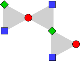
Figure 1: Vertices in our networks come in three types, represented here by the red circles, green diamonds, and blue squares, and are connected by three-way hyperedges that each join together exactly one circle, one diamond, and one square. In the language of folksonomies, the circles represent, say, the resources, the diamonds the tags, and the squares the users.

In this paper, we study the theory of such tripartite graphs, starting with basic network properties such as degree distributions and then developing a random graph model that allows us to make analytic predictions of a variety of network properties. We test our predictions by comparing them with data from the Flickr folksonomy and find good agreement in some, but not all, cases.

II Tripartite graphs

We begin our study of tripartite hypergraphs by outlining some of the basic properties of such networks. Our tripartite graphs have three different types of vertices, which, to preserve generality, we will refer to as red, green, and blue vertices. (In this paper, when discussing applications of the theory to folksonomies, red will represent resources, green tags, and blue users, but the theory itself is entirely agnostic about what the colors represent.) Let us suppose that there are $n_{r}$ red vertices, $n_{g}$ green ones, and $n_{b}$ blue ones.

The edges in our network are three-way hyperedges that each connect one red, one green, and one blue vertex. (We might say that the hyperedges are “colorless” or “white,” since red, green, and blue make white when combined in the human visual system.) Let us suppose there to be $m$ hyperedges in total.

There are a number of ways in which vertex degree can be defined for a hypergraph. Some authors, for instance, have defined degree as the total number of other vertices to which a given vertex is connected by hyperedges. This corresponds to the definition of degree in an ordinary graph (at least when there are no multiedges or self-edges), but in failing to distinguish between the different types of vertices to which hyperedges are connected, it can lead to confusion in the hypergraph case. The best, and also simplest, definition of degree for a vertex in a hypergraph is simply the number of hyperedges attached to that vertex. Thus a red vertex participating in four hyperedges has degree four. This might mean that it has four green and four blue neighbors in the network, but it is also possible that some neighboring vertices are common to more than one hyperedge, in which case the number of neighboring vertices of a given color may be smaller than four.

The mean degree $c_{r}$ of a red vertex in our network is given by the number of hyperedges in the network divided by the number of red vertices, and similarly for green and blue:

$$c_{r}={m\over n_{r}},\qquad c_{g}={m\over n_{g}},\qquad c_{b}={m\over n_{b}}.$$ (1)

Rearranging these equations to give three separate expressions for $m$, we also have,

$$n_{r}c_{r}=n_{g}c_{g}=n_{b}c_{b}=m.$$ (2)

Thus the mean degrees of the different vertex types cannot be chosen independently, but are linked via the fact that the same hyperedges connect to the red, green and blue vertices.

One of the most important parameters of a network is its degree distribution. Just as bipartite networks have two distinct degree distributions, our tripartite ones have three: we define $p_{r}(k)$ to be the fraction of red vertices in the network that have degree $k$, and $p_{g}(k)$ and $p_{b}(k)$ to be the corresponding quantities for green and blue vertices. These distributions satisfy the sum rules

$$\sum_{k=0}^{\infty}p_{r}(k)=\sum_{k=0}^{\infty}p_{g}(k)=\sum_{k=0}^{\infty}p_{b}(k)=1,$$ (3)

and

$$\sum_{k=0}^{\infty}kp_{r}(k)=c_{r},\quad\sum_{k=0}^{\infty}kp_{g}(k)=c_{g},\quad\sum_{k=0}^{\infty}kp_{b}(k)=c_{b}.$$ (4)

As with bipartite graphs, it is sometimes convenient to form “projections” of tripartite graphs onto a subset of their vertices. In a bipartite graph of red and green vertices, for instance, one forms a projection onto the red vertices alone by constructing the network of red vertices in which vertices are connected by an edge if they share a common green neighbor in the original bipartite graph Newman et al. (2001).

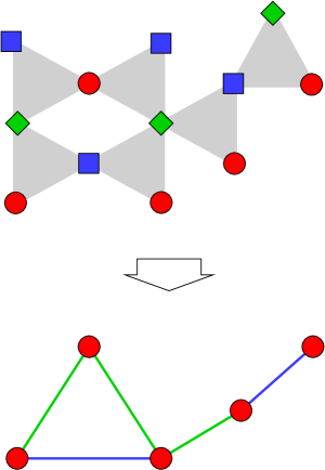
Figure 2: Ways of projecting a tripartite graph onto one of its vertex types (red in this case). Red vertices in the projected graph can be connected if they share a green neighbor (green edges in the projected graph), a blue neighbor (blue edges), or a neighbor of either kind (all edges together).

While for bipartite graphs there is essentially only one way of performing projections, there are several distinct possibilities for tripartite graphs—see Fig. 2. One can again join two red vertices if they share a green neighbor—in our Flickr example from the introduction, two photos would be connected if they have a tag in common. Or one can join two red vertices that share a common blue neighbor—two photos that were tagged by the same user. Or one could join vertices that share either a green or a blue neighbor. And of course one can define the equivalent projections onto the green and blue vertices.

But it doesn’t stop there. In a tripartite network, one can also form projections onto two of the colors. For instance, one can form a projected bipartite network of red and green vertices, in which a red and a green vertex are connected by an ordinary edge if they were connected by a hyperedge in the original network. Thus one can create a network of, for example, photos and the tags applied to them, while dropping information about which users applied which tags. And again one can also construct the equivalent projections onto red/blue and blue/green vertex combinations. Alternatively, one can construct a red/green network by connecting any pair of vertices—of different colors or not—if they share a common blue neighbor. Thus a tag would be connected to a photo if any user applied that tag to that photo, but tags would also be connected to other tags that were used by the same user.

Many other standard concepts in the theory of networks can be generalized to tripartite graphs, including clustering coefficients, correlations between the degrees of adjacent vertices (including three-point correlations), community structure and modularity, motif counts, and more. The concepts introduced above, however, will be sufficient for our purposes in this paper.

III Random tripartite graphs

In theoretical studies of networks, random graph models have received particular emphasis because they capture many of the essential properties of networked systems in the real world while simultaneously being amenable to analytic treatment. A variety of random graph models have been studied, from models of simple undirected or directed graphs to more complicated examples with correlations, communities, or bipartite structure Erdős and Rényi (1960); Molloy and Reed (1995); Bollobás (2001); Newman et al. (2001); Newman (2002). In this section we develop the theory of random tripartite hypergraphs with given degree distributions, which turn out to model many of the properties of real tripartite graphs quite effectively.

III.1 The model

Consider a model hypergraph with $n_{r}$ red vertices, $n_{g}$ green vertices, and $n_{b}$ blue vertices. Each vertex is assigned a degree, corresponding to the number of hyperedges it will have. These degrees can be visualized as “stubs” of hyperedges emerging from each vertex in the appropriate numbers. The degrees must satisfy Eq. (2), so that the total number of stubs emerging from vertices of each color is the same and equal to the total desired number of hyperedges $m$.

A total of $m$ three-way hyperedges are now created by choosing trios of stubs uniformly at random, one each from a red, green, and blue vertex, and connecting them to form hyperedges. This model is the equivalent for our tripartite graph of the so-called “configuration model” for unipartite graphs Molloy and Reed (1995) and the random bipartite graph model of Newman et al. (2001) for bipartite graphs.

Given the definition of the model, we can, for example, calculate the probability that a hyperedge exists between a given trio of vertices $i,j,k$. In the process of creating a single hyperedge, the probability that we will choose a specific stub attached to red vertex $i$ is $1/m$, since there are a total of $m$ stubs attached to red vertices and we choose uniformly among them. If $i$ has degree $k_{i}$ then the total probability of choosing a stub from vertex $i$ is $k_{i}/m$. Similarly the probability of choosing stubs from green and blue vertices $j$ and $k$ are $k_{j}/m$ and $k_{k}/m$. Given that there are $m$ hyperedges in total, the overall probability of a hyperedge between $i$, $j$, and $k$ is then

$$P_{ijk}=m\times{k_{i}\over m}\times{k_{j}\over m}\times{k_{k}\over m}={k_{i}k_{j}k_{k}\over m^{2}}.$$ (5)

Via a similar argument, the probability that there is a hyperedge connecting a particular red/green pair $i,j$ (or any other color combination) is $k_{i}k_{j}/m$. Note that in a sparse graph in which the typical degrees remain constant as the size of the graph increases, both of these probabilities vanish as $1/m$. Among other things, this implies that the chance of occurrence of small loops in the network vanishes in the limit of large graph size. In the language of graph theory, one says that the network is locally tree-like, a property that will be important in the developments to follow.

Rather than specifying the degree of every vertex in the network, we can alternatively specify just the degree distributions $p_{r}(k)$, $p_{g}(k)$, and $p_{b}(k)$ of the three vertex types (constrained to satisfy the sum rules (3) and (4)), then draw a specific sequence of degrees from those distributions and connect the vertices as before. As a practical matter, if one wanted to generate actual example networks on a computer, one would need to ensure that the degrees satisfied Eq. (2), which in general they will not on first being drawn from the distributions. A simple strategy for ensuring that they do is first to draw a complete set of degrees and then repeatedly choose at random a trio of vertices, one of each color, discard the current values of their degrees, and redraw them from the appropriate distributions until the constraint is satisfied.

The degree distributions represent the probability that a vertex of a given color chosen at random from the entire network has a given degree. If we choose a hyperedge at random, however, and follow it to the red, green, or blue vertex at one of its corners, that vertex will not have degree distributed according to $p_{r}(k)$, $p_{g}(k)$, or $p_{b}(k)$, and the reason is easy to see: vertices with many hyperedges are proportionately more likely to be encountered when following edges. A vertex of degree ten, for instance, has ten times as many chances to be chosen in this way than a similarly colored vertex of degree one. (And a vertex of degree zero will never be chosen at all.) Thus the distribution of degrees of vertices encountered is proportional to $kp_{r}(k)$ for red vertices, and similarly for green and blue. Requiring this distribution to sum to unity, the correctly normalized distribution is $kp_{r}(k)/\sum_{k}kp_{r}(k)=kp_{r}(k)/c_{r}$.

As in other random graph models, we are in fact usually interested not in the degree of the vertex we encounter but in the number of hyperedges attached to it other than the one we followed to reach it. This so-called excess degree, which is 1 less than the total degree, has the same distribution as above, but with the replacement $k\to k+1$, giving an excess degree distribution of

$$q_{r}(k)={(k+1)p_{r}(k+1)\over c_{r}},$$ (6)

and similarly for other vertex colors.

III.2 Generating functions

The fundamental tools we will use in calculating the properties of the random tripartite graph are probability generating functions. We begin by defining generating functions for the degree distributions thus:

$$r_{0}(z) =\sum_{k=0}^{\infty}p_{r}(k)z^{k},$$ (7a)

$$g_{0}(z) =\sum_{k=0}^{\infty}p_{g}(k)z^{k},$$ (7b)

$$b_{0}(z) =\sum_{k=0}^{\infty}p_{b}(k)z^{k}.$$ (7c)

Given these generating functions we can, for instance, easily calculate the means of the distributions: $c_{r}=r_{0}^{\prime}(1)$ and so forth. Higher moments are also straightforward.

We also define corresponding generating functions for the excess degree distributions:

$$r_{1}(z)=\sum_{k=0}^{\infty}q_{r}(k)z^{k}={1\over c_{r}}\sum_{k=0}^{\infty}(k+1)p_{r}(k+1)z^{k}={r_{0}^{\prime}(z)\over r_{0}^{\prime}(1)},$$ (8a)

and

$$g_{1}(z) =\sum_{k=0}^{\infty}q_{g}(k)z^{k}={g_{0}^{\prime}(z)\over g_{0}^{\prime}(1)},$$ (8b)

$$b_{1}(z) =\sum_{k=0}^{\infty}q_{b}(k)z^{k}={b_{0}^{\prime}(z)\over b_{0}^{\prime}(1)}.$$ (8c)

III.3 Projections

As a first example, we use our generating functions to calculate the degree distribution for the projection of a tripartite random graph onto one of its vertex types, as described in Section II. Consider first the projection onto (say) red vertices in which two red vertices are joined by an edge if they share a green neighbor. (The blue vertices are ignored in this projection.)

Suppose a given red vertex A has $s$ green neighbors and each of those green neighbors has $t$ red neighbors other than vertex A. Given that $s$ is distributed according to $p_{r}(s)$ and $t$ is distributed according to $q_{g}(t)$, the probability $\rho_{g}(k)$ that A has exactly $k$ neighbors in the projected network is

$$\rho_{g}(k)=\sum_{s=0}^{\infty}p_{r}(s)\sum_{t_{1}=0}^{\infty}q_{g}(t_{1})\ldots\sum_{t_{s}=0}^{\infty}q_{g}(t_{s})\,\delta\biggl{(}k,\sum_{n=1}^{s}t_{n}\biggr{)},$$ (9)

where $\delta(i,j)$ is the Kronecker delta. Multiplying both sides by $z^{k}$ and summing over $k$, the generating function for this probability distribution is,

$$R_{g}(z) =\sum_{k=0}^{\infty}z^{k}\sum_{s=0}^{\infty}p_{r}(s)$$

$$\qquad{}\times\sum_{t_{1}=0}^{\infty}q_{g}(t_{1})\ldots\sum_{t_{s}=0}^{\infty}q_{g}(t_{s})\,\delta\biggl{(}k,\sum_{n=1}^{s}t_{n}\biggr{)}$$

$$=\sum_{s=0}^{\infty}p_{r}(s)\sum_{t_{1}=0}^{\infty}q_{g}(t_{1})\ldots\sum_{t_{s}=0}^{\infty}q_{g}(t_{s})z^{\sum_{n}t_{n}}$$

$$=\sum_{s=0}^{\infty}p_{r}(s)\sum_{t_{1}=0}^{\infty}q_{g}(t_{1})z^{t_{1}}\ldots\sum_{t_{s}=0}^{\infty}q_{g}(t_{s})z^{t_{s}}$$

$$=\sum_{s=0}^{\infty}p_{r}(s)\Biggl{[}\sum_{t=0}^{\infty}q_{g}(t)z^{t}\Biggr{]}^{s}=\sum_{s=0}^{\infty}p_{r}(s)\bigl{[}g_{1}(z)\bigr{]}^{s}$$

$$=r_{0}(g_{1}(z)).$$ (10)

We can also calculate the generating function for the projection in which two red vertices are connected by an edge if they share either a green or a blue neighbor. The probability for a vertex to have $k$ neighbors in this network is

$$\rho_{gb}(k) =\sum_{s=0}^{\infty}p_{r}(s)\sum_{t_{1}=0}^{\infty}q_{g}(t_{1})\ldots\sum_{t_{s}=0}^{\infty}q_{g}(t_{s})$$

$$\quad{}\times\sum_{u_{1}=0}^{\infty}q_{b}(u_{1})\ldots\sum_{u_{s}=0}^{\infty}q_{b}(u_{s})\,\delta\biggl{(}k,\sum_{n=1}^{s}(t_{n}+u_{n})\biggr{)},$$ (11)

and the corresponding generating function is

$$R_{gb}(z) =\sum_{k=0}^{\infty}z^{k}\sum_{s=0}^{\infty}p_{r}(s)\sum_{t_{1}=0}^{\infty}q_{g}(t_{1})\ldots\sum_{t_{s}=0}^{\infty}q_{g}(t_{s})$$

$$\quad{}\times\sum_{u_{1}=0}^{\infty}q_{b}(u_{1})\ldots\sum_{u_{s}=0}^{\infty}q_{b}(u_{s})\,\delta\biggl{(}k,\sum_{n=1}^{s}(t_{n}+u_{n})\biggr{)}$$

$$=\sum_{s=0}^{\infty}p_{r}(s)\Biggl{[}\sum_{t=0}^{\infty}q_{g}(t)z^{t}\Biggr{]}^{s}\Biggl{[}\sum_{u=0}^{\infty}q_{b}(u)z^{u}\Biggr{]}^{s}$$

$$=r_{0}(g_{1}(z)b_{1}(z)).$$ (12)

We can use this result to calculate, for instance, the average degree in the projected network, which is given by

$$R^{\prime}_{gb}(1)=r^{\prime}_{0}(1)\bigl{[}b^{\prime}_{1}(1)+g^{\prime}_{1}(1)\bigr{]}.$$ (13)

We will also use it in Section IV to compare predictions of the random graph model with real-world networks.

III.4 Formation and size of the giant component

In this section we examine the component structure of our model network, focusing on the giant component. As with all networks, if our tripartite network is sufficiently sparse—if it has very few edges for the given number of vertices—then vertices will be connected together only in small groups or small components. If, however, the number of edges is sufficiently high, then a fraction of the vertices will join together into a single large group, the giant component, with the remainder in small components. There is a phase transition with increasing density at which the giant component forms that is closely analogous to the phase transition in classical percolation.

There is more than one possible definition of a component in our tripartite network, but the simplest approach is to define it as a set of vertices of any colors that are connected via hyperedges such that every vertex in the set is reachable from every other by some path through the network. Thus the collection of vertices depicted in the top panel of Fig. 2 constitutes a component in this sense.

When viewed in the context of folksonomies, components, and particularly the giant component, play an important practical role. In a folksonomy such as that of Flickr, the photography web site, users can “surf” between photographs by traversing the hypergraph. A user can, for example, click on the tag associated with a photo and see a list of other photos with the same tag. Similarly a user can click on the name of another user and see a list of photos that user has tagged. The existence, or not, of a giant component in the network dictates whether this type of surfing is actually useful or not. If there is no giant component, then surfing users will find themselves restricted to the small set of photos, tags, and users in the component in which they start their surfing. But if there is a giant component then users will be able to surf to a significant fraction of all photos on the entire web site just by clicking on tags or users that seem interesting. The same considerations affect automated surfing by computerized “crawlers” that crawl web sites either to perform directed searches (so-called “spiders”) or to create indexes for later search. If there is no giant component in the folksonomy, then it cannot be crawled in a useful way.

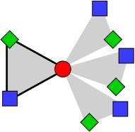
Figure 3: If a hyperedge (outlined in bold) is not to belong to the giant component, then it must be that none of the hyperedges reachable via, for instance, its red vertex are themselves members of the giant component.

We can calculate properties of the giant component in our tripartite random graph by methods similar to those used for ordinary random graphs Newman et al. (2001). Consider a randomly chosen hyperedge in the full hypergraph, as depicted in Fig. 3, and let us calculate the probability that this hyperedge is not a part of the giant component. We define $u_{r}$ to be the probability that the hyperedge is not connected to the giant component via its red vertex, and similarly for $u_{g}$ and $u_{b}$, so that the total probability of not belonging to the giant component is $u_{r}u_{g}u_{b}$.

Suppose that the excess degree of the red vertex—the number of other hyperedges attached to it—is $k$. (In the example shown in Fig. 3 we have $k=3$.) In order that the hyperedge be not connected to the giant component via the red vertex it must be that none of these other hyperedges are connected to the giant component either. Any one hyperedge satisfies this criterion with probability $u_{g}u_{b}$—the probability that neither of its other corners lead to the giant component—and all $k$ of them together do so with probability $(u_{g}u_{b})^{k}$.

The excess degree is distributed according to the distribution $q_{r}(k)$ defined in Eq. (6). Averaging over this distribution, we then derive an expression for $u_{r}$ thus:

$$u_{r}=\sum_{k=0}^{\infty}q_{r}(k)(u_{g}u_{b})^{k}=r_{1}(u_{g}u_{b}).$$ (14)

Similarly we can show that

$$u_{g}=g_{1}(u_{b}u_{r}),\qquad u_{b}=b_{1}(u_{r}u_{g}).$$ (15)

The simultaneous solution of these three equations for $u_{r}$, $u_{g}$, and $u_{b}$ then allows us to calculate the probability $1-u_{r}u_{g}u_{b}$ that a randomly chosen hyperedge is in the giant component. Alternatively, the probability that a randomly chosen red vertex is not in the giant component is the probability that none of its $k$ hyperedges lead to the giant component, which is $\sum_{k}p_{r}(k)(u_{g}u_{b})^{k}=r_{0}(u_{g}u_{b})$, so the that a red vertex is in the giant component with probability

$$S_{r}=1-r_{0}(u_{g}u_{b}),$$ (16)

and we can write similar equations for $S_{g}$ and $S_{b}$. $S_{r}$ can also be thought of as the fraction of red vertices in the giant component, and hence is a measure of the size of that component. The absolute number of red vertices in the giant component is $n_{r}S_{r}$ and the number of vertices of all colors is $n_{r}S_{r}+n_{g}S_{g}+n_{b}S_{b}$.

As in other random graph models, it is in most cases not possible to solve Eqs. (14) and (15) for $u_{r}$, $u_{g}$, and $u_{b}$ in closed form, but a numerical solution can be found easily by iteration starting from suitable initial values.

We can also derive a condition for the existence of a giant component in the network. A giant component exists if and only if $u_{r}$, $u_{g}$, and $u_{b}$ are all less than 1. (They must all be less than 1 because an extensive giant component of vertices of any one color automatically implies an extensive component of the other two colors, since, with only mild conditions on the degree distribution, the first color must be connected into a giant component by an extensive number of hyperedges, and each hyperedge is attached to one vertex of each color.)

Consider values of the variables that are only slightly different from 1 thus:

$$u_{r}=1-\epsilon_{r},\qquad u_{g}=1-\epsilon_{g},\qquad u_{b}=1-\epsilon_{b},$$ (17)

where $\epsilon_{r}$, $\epsilon_{g}$, and $\epsilon_{b}$ are small. Then, from Eq. (14),

$$\epsilon_{r} =1-u_{r}=1-r_{1}(u_{g}u_{b})=1-r_{1}(1-\epsilon_{g}-\epsilon_{b}+\epsilon_{g}\epsilon_{b})$$

$$=(\epsilon_{g}+\epsilon_{b})r_{1}^{\prime}(1)+\mathrm{O}(\epsilon^{2}),$$ (18)

where we have performed a Taylor expansion of $r_{1}$ and made use of $r_{1}(1)=1$ (which is necessarily true if $q_{r}(k)$ is a properly normalized distribution). We can derive similar equations for $\epsilon_{g}$ and $\epsilon_{b}$ and combine all three into the single vector equation

$$\begin{pmatrix}\epsilon_{r}\\ \epsilon_{g}\\ \epsilon_{b}\end{pmatrix}=\begin{pmatrix}0&r&r\\ g&0&g\\ b&b&0\end{pmatrix}\begin{pmatrix}\epsilon_{r}\\ \epsilon_{g}\\ \epsilon_{b}\end{pmatrix},$$ (19)

where we have introduced the shorthand $r=r_{1}^{\prime}(1)$, $g=g_{1}^{\prime}(1)$, and $b=b_{1}^{\prime}(1)$.

If $u_{r}$, $u_{g}$, and $u_{b}$ are to be less than 1, meaning the corresponding $\epsilon$’s must all be non-zero, then this equation implies the determinant condition

$$\begin{vmatrix}-1&r&r\\ g&-1&g\\ b&b&-1\end{vmatrix}=0,$$ (20)

or

$$2rgb+rg+gb+br=1.$$ (21)

This condition defines the point at which the phase transition takes place. Equivalently, $2rgb+rg+gb+br$ crosses 1 at the transition. In fact it is greater than 1 when there is a giant component and less 1 when there is none (rather than the other way around) as can be shown by exhibiting any example where this is the case. A suitable example is provided by a network in which all vertices have degree one, which clearly has no giant component. This choice makes $r=g=b=0$ and the result follows.

Thus our condition for the existence of a giant component is,

$$2rgb+rg+gb+br>1.$$ (22)

This is the equivalent of the well known condition of Molloy and Reed for the existence of a giant component in a unipartite random graph Molloy and Reed (1995).

An alternative form for this condition can be derived by making use of Eqs. (6) and (8) to write

$$r =r_{1}^{\prime}(1)=\sum_{k=0}^{\infty}kq_{r}(k)={1\over c_{r}}\sum_{k=0}^{\infty}k(k+1)p_{r}(k+1)$$

$$={1\over c_{r}}\sum_{k=0}^{\infty}k(k-1)p_{r}(k)={\langle k^{2}\rangle_{r}\over\langle k\rangle_{r}}-1,$$ (23)

and similarly for $g$ and $b$. Here $\langle\ldots\rangle_{r}$ indicates an average over the degree distribution of the red vertices and $c_{r}=\langle k\rangle_{r}$.

Substituting these expressions into (22), we find, after some algebra, that

$${\langle k\rangle_{r}\over\langle k^{2}\rangle_{r}}+{\langle k\rangle_{g}\over\langle k^{2}\rangle_{g}}+{\langle k\rangle_{b}\over\langle k^{2}\rangle_{b}}<2.$$ (24)

This form is particularly pleasing, since it has the same general shape as the criterion of Molloy and Reed for the unipartite case, which can be written as $\langle k\rangle/\langle k^{2}\rangle<\frac{1}{2}$.

III.5 Other types of components

The definition of a component used in the previous section is not the only one possible for our tripartite graph. In some folksonomies one cannot surf over connections formed by both users and tags. In some cases, for instance, one is barred from seeing which resources a particular user has tagged for privacy reasons, meaning one can surf between resources with the same tag, but not with the same user. In this case we are surfing on the network formed by two colors of vertices only, say red and green.

We can approach this situation using the same techniques as in the previous section. We define probabilities $u_{r}$ and $u_{g}$ as before and find that they satisfy the equations,

$$u_{r}=r_{1}(u_{g}),\qquad u_{g}=g_{1}(u_{r}).$$ (25)

Linearizing around the point $u_{r}=u_{g}=1$ we then find that the transition at which the giant component appears takes place when

$$\begin{vmatrix}-1&r\\ g&-1\end{vmatrix}=0,$$ (26)

or equivalently $rg=1$, with $r$ and $g$ defined as before. By considering appropriate special cases, one can then show that the giant component exists if and only if $rg>1$. Substituting from Eq. (23), we can also write this condition in the form,

$${\langle k\rangle_{r}\over\langle k^{2}\rangle_{r}}+{\langle k\rangle_{g}\over\langle k^{2}\rangle_{g}}<1.$$ (27)

Note that this expression is not symmetric with respect to permutations of the three color indices, as Eq. (24) was. This means that in general giant components for different color pairs will appear at different transitions, and it is possible to have a giant component for one pair without having a giant component for another. Thus for instance in our Flickr example one might be able to surf the network of photos and tags, but not the network of photos and users. (Actually, one can surf both just fine in the real Flickr network.)

III.6 Percolation

One can also consider percolation processes on tripartite networks. If some vertices are removed from the network then the remaining network may or may not percolate, i.e., possess a giant component. For example, on the Flickr web site users can designate photos as publicly viewable or not, and those that are not are, for all intents and purposes, removed from the network. One cannot use them, for instance, for surfing across the network. There are many ways in which vertices might be removed, but as a simple example let us assume that vertices of only one kind are removed and make the standard percolation assumption that they are removed uniformly at random. (More complicated percolation schemes are certainly possible, with more than one type of vertex removed, different probabilities of removal for different types, or nonuniform removal, and all of these schemes can be studied by methods similar to those outlined here.)

Suppose a fraction $\phi$ of the red vertices in our network are present (or functional) and $1-\phi$ are removed (or nonfunctional). In the language of percolation theory, a fraction $\phi$ of the vertices are occupied. Then define $u_{r}$ as before to be the probability that the red vertex attached to a random hyperedge does not belong to the giant component, or the giant cluster as it is more commonly called in the percolation context. There are two different ways in which this can happen. If the vertex itself has been removed, then it does not belong to the giant cluster. Alternatively, it may be present but, as before, none of its neighbors, either blue or green, are in the giant cluster. This allows us to write down an expression for $u_{r}$ thus:

$$u_{r}=1-\phi+\phi r_{1}(u_{g}u_{b}).$$ (28)

The corresponding expressions for $u_{g}$ and $u_{b}$ are the same as in our previous calculation, $u_{g}=g_{1}(u_{b}u_{r})$, $u_{b}=b_{1}(u_{r}u_{g})$, and the fractions of red, green, and blue vertices in the giant percolation cluster are

$$S_{r} =\phi[1-r_{0}(u_{g}u_{b})],$$ (29a)

$$S_{g} =1-g_{0}(u_{b}u_{r}),$$ (29b)

$$S_{b} =1-b_{0}(u_{r}u_{g}).$$ (29c)

We can also calculate an expression for the value of $\phi$ at which the percolation transition happens. As before we perturb around the point $u_{r}=u_{g}=u_{b}=1$ that corresponds to no giant cluster and the equivalent of Eq. (19) is

$$\begin{pmatrix}\epsilon_{r}\\ \epsilon_{g}\\ \epsilon_{b}\end{pmatrix}=\begin{pmatrix}0&\phi r&\phi r\\ g&0&g\\ b&b&0\end{pmatrix}\begin{pmatrix}\epsilon_{r}\\ \epsilon_{g}\\ \epsilon_{b}\end{pmatrix},$$ (30)

with $r$, $g$, and $b$ defined as before. This implies that the transition happens at $\phi=\phi_{c}$ where $\phi_{c}$ is the solution of $2\phi rgb+\phi rg+gb+\phi br=1$. That is,

$$\phi_{c}={1-gb\over r(2gb+g+b)}.$$ (31)

Making use of Eq. (23) and the corresponding expressions for $g$ and $b$ we then find that

$$\phi_{c}=\biggl{(}{\langle k^{2}\rangle_{r}\over\langle k\rangle_{r}}-1\biggr{)}^{-1}\biggl{[}\biggl{(}2-{\langle k\rangle_{g}\over\langle k^{2}\rangle_{g}}-{\langle k\rangle_{b}\over\langle k^{2}\rangle_{b}}\biggr{)}^{-1}-1\biggr{]}.$$ (32)

III.7 Simulations

Before looking at real-world tripartite networks, we first compare our calculations with simulation results for computer-generated random graphs.

Consider a tripartite random graph with Poisson degree distributions thus:

$$p_{r}(k)=\mathrm{e}^{-c_{r}}{c_{r}^{k}\over k!},\quad p_{g}(k)=\mathrm{e}^{-c_{g}}{c_{g}^{k}\over k!},\quad p_{b}(k)=\mathrm{e}^{-c_{b}}{c_{b}^{k}\over k!},$$ (33)

where the average degrees $c_{r}$, $c_{g}$, and $c_{b}$ satisfy Eq. (2). The corresponding generating functions are

$$r_{0}(z) =r_{1}(z)=\mathrm{e}^{-c_{r}}\sum_{k=0}^{\infty}\frac{c_{r}^{k}}{k!}z^{k}=\mathrm{e}^{c_{r}(z-1)},$$

$$g_{0}(z) =g_{1}(z)=\mathrm{e}^{-c_{g}}\sum_{k=0}^{\infty}\frac{c_{g}^{k}}{k!}z^{k}=\mathrm{e}^{c_{g}(z-1)},$$

$$b_{0}(z) =b_{1}(z)=\mathrm{e}^{-c_{b}}\sum_{k=0}^{\infty}\frac{c_{b}^{k}}{k!}z^{k}=\mathrm{e}^{c_{b}(z-1)}.$$ (34)

We can use these to calculate, for instance, the degree distribution of the projection of the network onto the red vertices in which two vertices are connected if they share either a green or a blue neighbor. The generating function for this distribution is given by Eq. (12) to be

$$R_{gb}=r_{0}(g_{1}(z)b_{1}(z))=\mathrm{e}^{c_{r}(\mathrm{e}^{(c_{g}+c_{b})(z-1)}-1)}.$$ (35)

Expanding in powers of $z$, we then find that the probability $\rho_{gb}(k)$ of a red vertex having exactly $k$ neighbors in the projected network is

$$\rho_{gb}(k) ={(c_{g}+c_{b})^{k}\over k!}\mathrm{e}^{c_{r}(\mathrm{e}^{-(c_{g}+c_{b})}-1)}$$

$$\qquad{}\times\sum_{m=1}^{k}\biggl{\{}{\!{k\atop m}\!}\biggr{\}}\bigl{[}c_{r}\mathrm{e}^{-(c_{g}+c_{b})}\bigr{]}^{m},$$ (36)

where $\bigl{\{}{k\atop m}\bigr{\}}$ is a Stirling number of the second kind, i.e., the number of ways of dividing $k$ objects into $m$ nonempty sets Abramowitz and Stegun (1974).

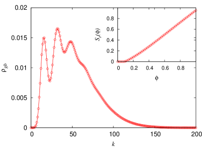
Figure 4: The degree distribution for the projection of our Poisson hypergraph onto its red vertices alone, in which two red vertices are joined by an edge if they have either a green or a blue neighbor in common on the original tripartite network. The solid line is the exact solution, Eq. (36), and the points are the results of numerical simulations averaged over a hundred realizations of the network. The error bars are smaller than the size of the points in all cases. Inset: The fraction of red vertices belonging to the giant percolation cluster for site percolation on the tripartite network, as a function of occupation probability $\phi$. The solid line is the exact solution and the points are the results of numerical simulations.

The main panel of Fig. 4 shows the form of this distribution for the case $c_{r}=3$, $c_{g}=10$, $c_{b}=6$. In the same plot we show the results of simulations in which random tripartite graphs with the same degree distributions and $n_{r}=100\,000$, $n_{g}=30\,000$, and $n_{b}=50\,000$ were generated and then explicity projected onto the red vertices and the resulting degree distribution measured directly. As the figure shows, the agreement between the two is excellent.

The inset of Fig. 4 shows the size of the giant cluster for percolation on the red vertices of the same network as a function of the occupation probability $\phi$, calculated both by numerical solution of Eqs. (28)–(29) and by direct measurement on simulated networks. Again the agreement is excellent.

IV Comparison with real-world data

In this section we compare the predictions of our tripartite random graph model against data for the folksonomy of the Flickr photo-sharing web site. As we show, the theory and empirical observations agree well in some respects, but less well in others. In many ways the discrepancies are at least as interesting as the cases of agreement, since they indicate situations in which the structure of the observed network cannot be explained by a simple random model that ignores social and other effects. When data and model disagree it is a sign that these effects are important in determining the network structure. Thus, as with other random graph models, one of the most significant roles our model can play may be as a null model that allows the experimenter to determine when a network is doing something nontrivial.

Our example data set represents the folksonomy network of $266\,198$ photos added to the Flickr web site by its users during 2007, along with the tags applied to those photos and the users who applied them. The first step in analyzing the data is to measure the three degree distributions for the three types of vertices. The degree distributions are shown in Fig. 5. As is common in most social networks, they are highly right-skewed, meaning there are many vertices of low degree and a small number of very high degree, although the distributions do not follow power-law forms as the distributions in some networks do. Using these distributions, we can, following Eqs. (7) and (8), construct the corresponding generating functions, which are simple polynomials (albeit of high order) that can be easily evaluated numerically.

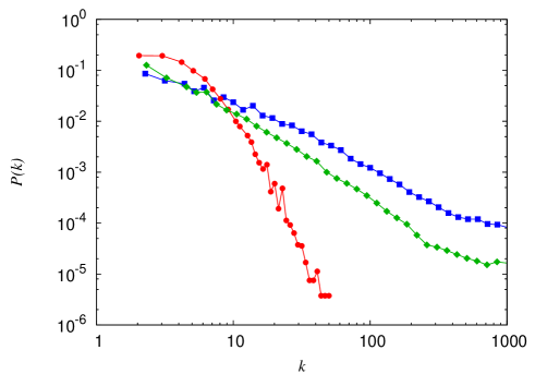
Figure 5: The three degree distributions of the tripartite Flickr folksonomy network for photos (red), tags (green), and users (blue).

We can use our generating functions to calculate, for example, the generating functions $R_{gb}(z)$ and so forth for the degree distributions of the projections of the network onto one vertex type, using Eqs. (10) and (12) and their equivalents for other vertex types. Again these functions can be rapidly evaluated for any argument $z$ numerically. The degree distributions themselves are then given by derivatives of the generating functions thus:

$$p_{k}=\frac{1}{k!}\frac{\mathrm{d}^{k}R_{gb}}{\mathrm{d}z^{k}}\biggr{|}_{z=0}.$$ (37)

Direct numerical evaluation of derivatives is plagued by problems with noise and should be avoided, but one can get good results Moore and Newman (2000) by instead employing Cauchy’s integral formula for the $k$th derivative of a function:

$$\frac{\mathrm{d}^{k}\!f}{\mathrm{d}z^{k}}\biggr{|}_{z=z_{0}}=\frac{k!}{2\pi\mathrm{i}}\oint\frac{f(z)}{(z-z_{0})^{k+1}}\>\mathrm{d}z,$$ (38)

where the integral is around a contour enclosing the point $z_{0}$ but excluding any poles of $f(z)$. Applying this formula to (37) we get

$$p_{k}=\frac{1}{2\pi\mathrm{i}}\oint\frac{R_{gb}(z)}{z^{k+1}}\>\mathrm{d}z.$$ (39)

We then calculate the degree distribution by performing the contour integral numerically around a suitable contour (the unit circle $|z|=1$ works well). One can without difficulty calculate to good precision the first thousand or so coefficients of the generating function in this fashion.

We have performed this calculation using the degree distributions of the Flickr network and projecting onto the resources, i.e., the photos. Figure 6 shows a comparison of the results with the degree distribution for the actual projected network. The upper solid line in the figure represents the theoretical result, while the circles represent the measurements. Although the two curves have the same general shape, it’s clear from the figure that the agreement between them is only moderately good in this case. Upon closer inspection, however, it turns out that there is a relatively simple reason for this.

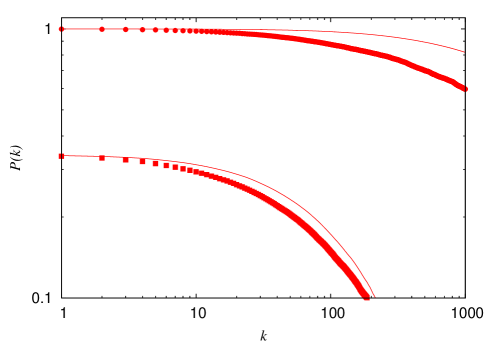
Figure 6: Circles show the cumulative distribution function for the degree distribution of the projection of the Flickr network onto its photograph vertices, while the upper solid line shows the predictions of the random graph model for the same quantity. Squares show the same function after pruning of the data to remove multiple tagging as described in the text and the lower solid curve shows the corresponding model prediction, recalculated from the new degree distributions after pruning.

As discussed in Section III.1, our random graph model assumes a locally-tree like structure for the tripartite network, a structure with no short loops. The Flickr network, on the other hand, turns out to have many short loops, which is why empirical measurements and model do not agree in Fig. 6. As we now show, however, the loops in the Flickr network are primarily of a trivial kind that can easily be allowed for in the calculations.

Typically, photos are not added to the Flickr network individually, but in sets. The most common practice is for a user to upload a set of photos on a particular subject—say, pictures of a Ferrari motor car—and then label all of the photos in the set with the same set of tags—Ferrari, automobile, sports car, and so forth. This creates short loops between photos in the set of the form $P_{1}\to T_{1}\to P_{2}\to T_{2}\to P_{1}$, where the $P$s are the photos and the $T$s are tags. These loops will have an adverse affect on the calculation of the number of neighbors a photo has in the projected network, since in many cases two projected edges from a photo will lead to the same neighboring photo, rather than to different neighbors, and hence give a lower degree in the projected network than our naive random graph calculation.

To test the effect of these “trivial” loops in the network structure, we have pruned the data set to remove instances of multiple tagging. In the pruned data set the application by a user of many tags to the same photo is represented by just a single hyperedge, rather than many. In this representation, hyperedges represent the act of tagging a photo, rather than a specific tag, and only one hyperedge is included between a user and a photo no matter how many tags the user applies. Similarly we also represent the tagging of many photos with the same tag by a single hyperedge, so that hyperedges represent the act of tagging an entire photo set, rather than just a single photo. This should remove most instances of trivial loops in the projected network of the type described above.

Now we calculate again the projection of the hypergraph onto the set of photos. We also recalculate the theoretical predictions to reflect the changed degree distributions of the hypergraph following pruning. The results are shown in Fig. 6 (squares and lower solid curve) and, as the figure shows, the agreement is now quite good between theory and observation. This suggests that the earlier disagreement between the two is indeed primarily a result of the presence of the loops in the hypergraph introduced by the practice of multiple tagging.

We can perform similar calculations for projections onto other types of vertices. In Fig. 7 we show degree distributions, before and after pruning of the data set, for the projection onto users. Agreement between theory and observation for the unpruned data is again quite poor in this case but significantly better for the pruned data.

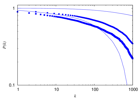
Figure 7: Cumulative distribution functions for the degree distributions of the projection of the Flickr network onto its user vertices, both before and after pruning of the data. The points represent the observations, unpruned (circles) and pruned (squares), while the solid lines represent the predictions of the model.

These calculations provide, in many ways, a good example of the utility of random graph models. When compared with the raw data from the Flickr network, our random graph model agrees qualitatively, but not quantitatively, indicating that there are effects present in the network that are not accounted for by simple random hyperedges. On the other hand, once one prunes the data to remove multiple tagging, the agreement becomes much better, suggesting that multiple tagging is the primary nonrandom behavior taking place in the network and that in other respects the network is in fact quite close to being a random graph. Thus the model allows us not only to say when the network deviates from the random assumption, but also the particular nature of the deviation.

V Conclusions

Motivated by the emergence of new types of social networks, such as folksonomies, we have in this paper proposed and studied a model of random tripartite hypergraphs. We have defined basic network measures, such as degree distributions and projections onto individual vertex types, and calculated a variety of statistical properties of the model in the limit of large network size. Among other things we have calculated the explicit degree distributions for projected networks, conditions for the emergence of a giant component, the size of the giant component when there is one, and the location of the percolation threshold for site percolation on the network. In principle, the techniques introduced could be extended to hypergraphs with more vertex types or additional types of edges, although we have not pursued any such extensions here.

We have compared our results against measurements of computer-generated random hypergraphs and a real-world tripartite network, the folksonomy of the on-line photo-sharing web site Flickr. In the latter case, we have focused on the degree distributions of projections of the hypergraph onto one vertex type and find that in some instances the theory makes predictions in moderately good agreement with the observations while in others the agreement is poorer. In all cases, however, we find that agreement becomes significantly better when we remove instances of multiple tagging from the network—instances in which a user applies many tags to the same photo or the same tag to many photos—suggesting that the disagreement is primarily a result of relatively trivial structures in the network, rather than more subtle or large-scale social network effects.