AGN Jet-induced Feedback in Galaxies.
II. Galaxy colours from a multicloud simulation

Abstract

We study the feedback from an AGN on stellar formation within its host galaxy, mainly using one high resolution numerical simulation of the jet propagation within the interstellar medium of an early-type galaxy. In particular, we show that in a realistic simulation where the jet propagates into a two-phase ISM, star formation can initially be slightly enhanced and then, on timescales of few million years, rapidly quenched, as a consequence both of the high temperatures attained and of the reduction of cloud mass (mainly due to Kelvin-Helmholtz instabilities). We then introduce a model of (prevalently) negative AGN feedback, where an exponentially declining star formation is quenched, on a very short time scale, at a time $t_{AGN}$, due to AGN feedback. Using the Bruzual & Charlot (2003) population synthesis model and our star formation history, we predict galaxy colours from this model and match them to a sample of nearby early-type galaxies showing signs of recent episodes of star formation (Kaviraj et al. 2007). We find that the quantity $\mbox{$t_{gal}$}-\mbox{$t_{AGN}$}$, where $t_{gal}$ is the galaxy age, is an excellent indicator of the presence of feedback processes, and peaks significantly around $\mbox{$t_{gal}$}-\mbox{$t_{AGN}$}\approx 0.85\,\rm Gyr$ for our sample, consistent with feedback from recent energy injection by AGNs in relatively bright ($M_{B}\mathrel{\hbox to0.0pt{\lower 3.5pt\hbox{\hskip 0.5pt$\sim$}\hss}\raise 0.5pt\hbox{$<$}}-19$) and massive nearby early-type galaxies. Galaxies that have experienced this recent feedback show an enhancement of 3 magnitudes in $NUV(GALEX)-g$, with respect to the unperturbed, no-feedback evolution. Hence they can be easily identified in large combined near UV-optical surveys.

1 Introduction

Active galactic nuclei (AGN) have been advocated in recent years as sources able to influence the evolutionary history of stellar populations within their host galaxies. They are ubiquitous and lie in the cores of a wide variety of galaxies, possibly suppressing, or possibly on occasion speeding up, star formation (SF). Massive and bright early-type galaxies (ETGs) have been shown to host very old stellar populations where SF stopped early, while fainter ETGs show lower ages and more protracted SF phases (Thomas et al. 2005, De Lucia et al. 2006). This is the so-called downsizing scenario, which is predicted by observations and generated in some recent simulations (Cowie et al. 1996, Borch et al. 2006, Bundy et al. 2006, De Lucia et al. 2006, Trager 2000, Thomas et al. 2005, 2005, Tortora et al. 2009). However, only very recently semi-analytic simulations have been able to reproduce some of the key observations (Cattaneo et al. 2006, De Lucia et al. 2006).

Kauffmann & Charlot (1998) predicted results that contrast with the downsizing scenario. The main reason for this discrepancy may be that supernova feedback in massive galaxies is not sufficient to quench SF (Dekel & Silk 1986, Benson et al. 2003). Feedback from AGN is the additional source able to heat the cold gas that fuels SF in galaxies. It is such effects that allow us to match the evolution of massive galaxies predicted from simulations with results from observations (e.g., Kaviraj et al. 2005, Silk 2005, Bower et al. 2006, Croton et al. 2006, De Lucia et al. 2006). However, these studies did not account for the downsizing phenomenon.

Feedback from AGN plays a major role during different phases of galaxy evolution. Higher activity is observed at high redshifts. At these early phases of galaxy evolution, during a major merger, the gas accreted by central supermassive black holes is ejected within the host galaxy, and inhibits SF (Di Matteo et al. 2005, Springel et al. 2005a, b). At more recent epochs, the effect of AGN feedback is weaker, but still sufficient to quench SF, particularly near the central regions (Croton et al. 2006, Bower et al. 2006, Schawinski et al. 2006, 2008). Evidence for the presence of AGNs is evident in many previous studies. In particular, Kauffmann et al. (2003) collected more than 20000 narrow-line AGNs from SDSS at $z\mathrel{\hbox to0.0pt{\lower 3.5pt\hbox{\hskip 0.5pt$\sim$}\hss}\raise 0.5pt\hbox{$<$}}0.3$. Type-II AGN are found within host galaxies having structural properties similar to normal ETGs, and reside almost exclusively in massive galaxies with $M_{\star}>10^{10}\,\rm M_{\odot}$. Many of these galaxies have experienced a recent burst of SF or show evidence of ongoing SF, thus indicating that a black hole and prominent source of fuel supply are necessary ingredients for AGN feedback, but no evidence of SF quenching is found (Kauffmann et al. 2003). While the existence of a black hole within massively star forming galaxies is a rarity in our cosmological neighbors, the situation is different at higher redshifts, where the AGN frequency is higher (Hasinger et al. 2005) and the feedback could be effective in producing red galaxies (Benson et al. 2003, Cattaneo et al. 2006, Schawinski et al. 2008).

More recently, a series of analyses have been devoted to the detection of recent star formation (RSF) within the last Gyrs of galaxy lifetimes. Ultraviolet data allowed the detection of small fractions of young stars, allowing one to trace this residual SF in ETGs both in the local universe (Yi et al. 2005, Kaviraj et al. 2007a) and at high redshift (Kaviraj et al. 2008). The link between SF and AGNs is strengthened by other analyses, where AGNs have been found to be responsible for the migration of star-forming galaxies, lying within the blue cloud, to almost quiescent located in the red sequence (Schawinski et al. 2006, 2007, 2008, Bildfell et al. 2008). In Kaviraj et al. (2007b), the recent feedback effect in E+A galaxies is analyzed and the bimodal correlation of the quenching efficiency with mass and luminosity is interpreted as due to negative feedback from supernovae or AGNs.

The physics of the SF-AGN connection is still poorly understood, and the empirical models of SF quenching by AGN used in different works (Granato et al. 2001, 2004, Martin et al. 2007a), although reasonable, do not yet have a solid motivation. Thus, a primary goal should be to analyze this phenomenology by means of hydrodynamical simulations, modelling the propagation of jets produced by AGNs within a gaseous medium (Scheuer 1974, Falle 1991) and their interaction with an inhomogeneous interstellar medium (2005, 2007, Sutherland & Bicknell 2007). In a previous paper (Antonuccio-Delogu & Silk 2008, paper I hereafter) we used an Adaptive Mesh Refinement (AMR) code to follow the evolution of the cocoon produced by the jet propagating in the ISM/IGM: we have analyzed the thermodynamic evolution of a cloud embedded within the cocoon and seen how its SF is modified. We found the SF to be quenched on time-scales of $10^{5}-10^{6}\,\rm yrs$.

In the present paper, we deduce a Star Formation History (hereafter SFH) directly from a numerical simulation of the interaction of an AGN with the multiphase ISM of its host galaxy. In principle, a realistic simulation should at least encompass a range of scales spanning more than 5 orders of magnitudes in the spatial coordinates, down to single star-formation scales, and should include a very wide range of heating and cooling phenomena. In this work we have restricted ourselves to consider only the mechanical feedback from the AGN, and its effect on the thermodynamic state of the ISM, thus neglecting the radiative feedback. We have modelled the ISM as a two-phase, multicloud system, and we have followed the thermodynamic evolution of both phases, particularly of the cold, star-forming phase. We introduce a feedback model where negative feedback, i.e. the suppression of SF within the volume affected by the jet, plays a dominant role. Using an empirical prescription to take into account the effect of cocoon on SF within cold clouds, we present a scenario where SF in unperturbed ETGs is described by an exponential SF law, corresponding to an early starburst followed by a slow decline. This evolution, starting at some time $t_{AGN}$ is quenched by a feedback process, and we follow the evolution of galaxy colors, determining the free parameters such as galaxy age $t_{gal}$ and $t_{AGN}$ by comparing with a previously studied sample (Kaviraj et al. 2007a).

For the first time, the amplitude and typical timescales of negative AGN feedback are directly derived from a simulation designed to address this phenomenology.

The plan of the paper is as follows. In Sect. 2 we discuss the simulation set-up, while in Sect. 3 we describe the propagation of the cocoon and its influence on SF. In order to compare predicted results with observations, we use single burst population models from Bruzual & Charlot (2003), suitably convolved with the SF rate predicted by our simulation: we describe our procedure and predicted synthetic colours in Sect. 4. Finally, Sect. 5 is devoted to a comparison with observations, and conclusions are detailed in Sect. 6.

Whenever required, we will adopt the 3-year WMAP “concordance” model: h=0.74,  $\Omega_{m}=0.234,\,\Omega_{b}h^{2}=0.0223$, corresponding to a Universe age of $t_{\rm Univ}\sim 13.6\,\rm Gyr$.

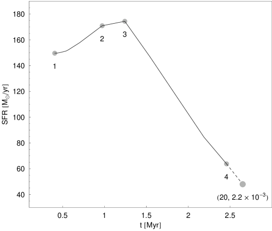
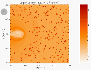
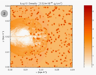
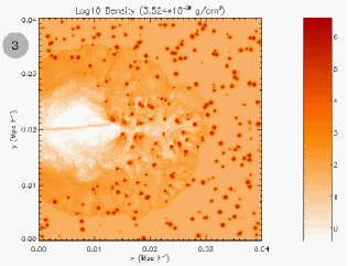
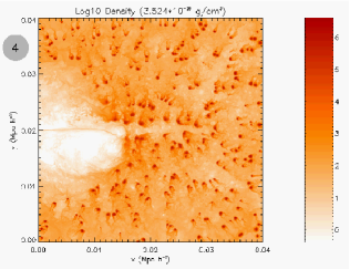
Figure 1: Temporal evolution of the star formation rate, for different snapshots of the simulation. In the upper panel we show the SF as a function of time (measured in $\mbox{$M_{\odot}$}\ /yr$ and $\rm Myr$ respectively), marking with numbers $1,\,2,\,3,\,4$ the SFs at the times $t\approx 0.4,\,1.0,\,1.2,\,2.5\,\rm Myr$ respectively. In the four bottom panels we show the propagation of the cocoon within the ISM and the effect on clouds (corresponding to the numbers in the top panel). SF rate is obtained using the Schmidt-Kennicutt law ($n=1.4$) and collecting the clouds within a radius of $27\,\rm kpc$. At very late epochs ($t\sim 20\,\rm Myrs$) the SFR declines to a very small value, as seen in the top panel. Note that our simulation maps only one-half of the galaxy, thus, assuming symmetry, we multiply our SF by a factor 2.

2 Simulation setup

To perform the simulation, we used FLASH v.2.5 (Fryxell et al. 2000), a parallel, Adaptive Mesh Refinement (AMR) code, which implements a second order, shock-capturing PPM solver. The modular structure of FLASH allows the inclusion of various physical effects, including a source of external heating, radiative cooling and thermal conduction. In our simulation, we include radiative cooling, using the standard cooling function from Sutherland & Dopita (1993), conveniently extended towards higher temperatures, $T>10^{7}\,\rm K$, which are attained within the cocoon generated in this simulation (see App. A in Paper I). We also take into account gravity, but we neglect thermal conduction and large-scale, ordered magnetic fields.

The jet is modelled as a one-component fluid, characterized by a density $\rho_{j}$ which is a fraction $\epsilon_{j}$ of the initial density of the interstellar medium. In order to prevent numerical instabilities at the jet/ISM injection interface, we use a steep, continuous and differentiable transverse velocity and density profile, as we did before (paper I; 2004, 2005):

$$v_{x,j}=\frac{V_{j}}{\cosh\left\{\left(\frac{y-y_{j}}{d_{j}}\right)^{\alpha_{j}}\right\}}$$ (1)

$$n_{j}=n_{env}-\frac{\left(n_{env}-n_{j}\right)}{\cosh\left\{\left(\frac{y-y_{j}}{d_{j}}\right)^{\alpha_{j}}\right\}}$$ (2)

where: $\alpha_{j}=10$ is an exponent which determines the steepness of the injection profile, $n_{j},n_{env}$ denote the jet and environment electron number densities and the scalelength $d_{j}$ characterizes the width of the jet. The power injected by the jet is then given by $P_{j}=\beta 2\pi d_{j}^{2}\rho_{j}V_{j}^{3}$, with $\beta\simeq 0.7158$. In this simulation we set: $P_{j}=10^{46}\,\rm erg\,s^{-1}$.

We model the environment, where the jet propagates, as a 2-phase interstellar medium, comprising a hot, diffuse, low-density component and a cold, clumped system of high density clouds in pressure equilibrium with the diffuse component. The warm phase is characterized by a density profile $\rho_{env}(r)$ and a constant temperature $T_{env}$. We assume that the diffuse gas is embedded within a dark matter halo, the latter being described by a NFW density profile. This DM halo is chosen to have a total mass $M_{h}=5\times 10^{11}\,{\rm M}_{\sun}$, concentration $c=10.2$ and a scalelength $l_{h}=206\,h^{-1}\,$ kpc. The ISM gas is assumed to be a fraction $m_{g}=\Omega_{gas}/\Omega_{DM}\approx 0.212$ of the DM, and to be distributed in hydrostatic equilibrium within this DM halo, following the prescription given in Appendix C of (2006). Each of the clouds in the cold component is modelled as a truncated isothermal sphere (TIS: Shapiro et al. 1999, 2001), because this model seems to adequately reproduce the properties of clouds formed in simulations of a thermally unstable ISM. TIS spheres posses a finite radius, and are characterized by two parameters, which we assume to be the mass $M_{cl}$ and a typical radius $r_{cl}$. They are exact solutions of the equilibrium equations for isothermal spheres confined by an external pressure. We distribute 300 clouds within the simulation volume, using a mass spectrum previously derived from numerical simulations (Baek et al. 2005). Summarizing, the simulation is specified by 10 parameters: three of these describe the DM halo ($M_{h},c,l_{h}$), two the diffuse phase of the ISM ($m_{g},T_{env}$), two the mass distribution within the cold component of the ISM ($M_{cl},r_{cl}$), and the last three describe the jet ($n_{j},d_{j},P_{j}$).

Table 1: Parameters of the simulation. The halo mass is in units of $M_{\sun}$, distances are measured in kpc $h^{-1}$, $n_{env},n_{j}$ are, respectively, the central gas electron and jet’s densities, in units of $\rm cm^{-3}$, $T_{env}$ is in Kelvin, $d_{j}$ and $P_{j}$ are the jet width and power, respectively. The latter is expressed in cgs units (ergs$\cdot$ sec.

Parameter	Adopted value
$M_{h}$	$5\times 10^{11}$
$c$	10.2
$l_{h}$	206
$m_{g}$	$1.06\times 10^{11}$
$n_{env}$	$10^{2}$
$T_{env}$	$10^{7}$
$n_{j}$	$1$
$d_{j}$	10
$P_{j}$	$10^{46}$

Figure 2: Star formation rate in 14 circular, equally-spaced shells. The results for different times are shown, from continuous to long dashed lines spanning $t=0.4,\,1,\,1.6,\,2.5,\,3.2\,\rm Myr$.

We choose a simulation box having a size: $L_{box}=40\,h^{-1}\,\rm kpc$, so that the jet will diffuse through it at the end of the simulation. The spatial resolution attained is a function of the maximum refinement level and of the structure of the code. For a block-structured AMR code like FLASH, where each block is composed by ${\rm n}_{x}\times{\rm n}_{y}$ cells, the maximum resolution along each direction is given by $L_{box}/({\rm n}_{x}2^{l})$, where $l$ is the maximum refinement level. In this simulation: ${\rm n}_{x}={\rm n}_{y}=8\,$ and $l=6$, thus the minimum resolved scale is $78.125\,$ pc. Note that we are performing a 2D simulation, but we do not impose any special symmetry.

We assume that the duty cycle of the jet is active for a time of $4\times 10^{6}$ yrs, as is typical for jets having such power (Shabala et al. 2008), and its power declines linearly with time since this epoch until it switches off at $t~{}\approx 2\times 10^{7}$ yrs. As for the star formation rate, we assume that the clouds are converting gas into stars with a rate specified by the Schmidt-Kennicutt (SK) law (Schmidt 1959, 1963, Kennicutt 1998): $SFR=\dot{\Sigma}=A\Sigma^{n}$, where $A=(2.5\pm 0.17)\times 10^{-4}\,\rm\mbox{$M_{\odot}$}\,yr^{-1}\,kpc^{-2}$ and $n=1.4\pm 0.15$. We further require that SF is ongoing only within regions having a mass larger than the Bonnor-Ebert mass (Ebert 1955, Bonnor 1956), and temperature less than a specified upper limit, i.e. $T\leq 1.2\times 10^{4}\,\rm K$. These are rather conservative constraints, which tend to underestimate the magnitude of the negative feedback.

Our initial setup is very different from that of the very recent simulation by Sutherland & Bicknell (2007), particularly in one very important point: while we model a population of pressure-confined clouds embedded within the ISM, Sutherland & Bicknell (2007) put a turbulent disk around the jet’s source, embedding the AGN within it, as they are more interested in addressing problems related to the evolution of GPS and CSS radio sources. Also, note that their simulation box is much smaller than ours (1 kpc), and the temporal scale is also very different ($\approx 10^{5}\,\rm yrs$ in their simulation, compared to $2\times 10^{7}\,\rm yrs$ in the present work). Moreover, one may notice that we have neglected the velocity field of the inhomogeneous component: in fact, as already noted by Sutherland & Bicknell (2007), for the spatial and temporal scales of interest, its inclusion has little effect on the evolution of the clouds and of their SF. The typical turbulent velocities of clouds are in the range $10-70\,{\rm km\,s}^{-1}$. Thus, on typical timescales $\mathrel{\hbox to0.0pt{\lower 3.5pt\hbox{\hskip 0.5pt$\sim$}\hss}\raise 0.5pt\hbox{$<$}}2\times 10^{7}\,\rm yrs$ in our simulation, these clouds have displacements $l\mathrel{\hbox to0.0pt{\lower 3.5pt\hbox{\hskip 0.5pt$\sim$}\hss}\raise 0.5pt\hbox{$<$}}0.2-1.4\,\rm kpc$, smaller than the average distance among clouds (see Fig. 1).

3 Propagation of the jet

Soon after the jet enters the ISM, a low-density region, the cocoon, is generated. The details of the propagation of the jet within the ISM, and the properties of the cocoon, have been extensively studied in the past (Scheuer 1974, Falle 1991). Only recently, however, numerical simulations have been used to study in more detail the effect which this interaction has on the inhomogeneous component of the ISM, where stars are forming (e.g., 2005, 2007). In Paper I, we extensively analyzed properties of cocoon and the interaction with a single cloud that is forming stars. In the following we will make few comments about cocoon propagation, concentrating rather on the effects on our multicloud system.

3.1 Quenching of star formation

The global evolution can be seen in Fig. 1, it is possible to distinguish two main phases, corresponding to the evolution of the cocoon: an active and passive phase. While the jet is active, the cocoon is fed and it expands almost self-similarly, while, when it is switched off, the cocoon diffuses and affects a larger fraction of the ISM.

Initially (see snapshots 1 and 2 in Fig. 1), the interaction mostly takes place through the weak shock at the interface between the cocoon and the ISM. This shock compresses and heats up the clouds, having two opposite effects on SF: compression tends to increase SF, but the larger temperature also increases the critical mass for gravitational collapse, thus decreasing the volume fraction of the clouds which can actively form stars. Globally, we observe an initial enhancement of SF (i.e., we observe a positive feedback). The effects of the two concomitant processes on clouds can be seen in Fig. 2, where we build the shell-SFs by adding the SF of clouds lying in a concentric annulus of mean radius $r$ and plot them as a function of radius for different time steps. Here, few episodes of positive feedback are evident in the clouds which are nearer to the cocoon. Later ( see snapshots 3 and 4 in Fig. 1), the cocoon propagates within the medium inducing a general increase of the temperature, which heats up the clouds and decreases their density, and finally the outer regions of the clouds are stripped due to Kelvin-Helmholtz instabilities, as we studied in more detail in Paper I. These effects tend to reduce the mass of the clouds, decreasing SF, and eventually drastically suppressing it on a time-scale of $2-3\times 10^{6}\,\rm yr$ (negative feedback). Obviously, the more external regions in the galaxy are affected later by the disruptive effect of the cocoon, being almost unperturbed until $t\sim 10^{6}\,\rm yr$ and $t=1.6\times 10^{6}\,\rm yr$, respectively at $r\sim 30$ and $\sim 45\,\rm kpc$ (see Fig. 2). As we see from this simulation, approximately on a timescale over which the cocoon diffuses, the clouds are destroyed: this is then the typical time-scale over which SF will be inhibited. Obviously, one must observe that this timescale is not exactly coincident with the duty cycle of the jet.

Figure 3: Timescale for feedback. The three curves refer to the same density profile, having $\rho_{0}=1.7\times 10^{-25}\,\rm g\,cm^{-3}$, $\beta=2$, and 3 values for $a_{0}=0.8,\,1,\,1.2\,\,\rm kpc\,h^{-1}$ (dashed, continuous and dotted curves, respectively). The strong dependence on $a_{0}$ is simply a consequence of the high exponent with which it appears in the expression for $t_{0}$.

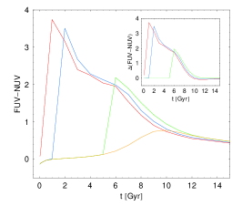
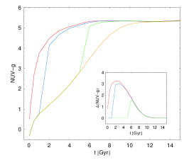
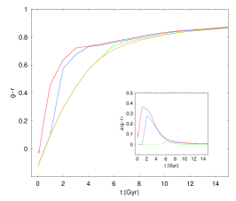
Figure 4: Estimated synthetic colours FUV-NUV, NUV-g and g-r (in AB system) as a function of galaxy age (in units of $\rm Gyr$) for $Z=\mbox{$Z_{\odot}$}$. Red, blue, green and orange curves correspond respectively to an unperturbed exponential SF with $\tau=0$, an exponential SF with $\tau=1\,\rm Gyr$ and $\mbox{$t_{AGN}$}=1\,\rm Gyr$, an exponential SF with $\tau=1\,\rm Gyr$ and $\mbox{$t_{AGN}$}=5\,\rm Gyr$ and an unperturbed exponential SF with $\tau=1\,\rm Gyr$. In the inset panels we show the difference of colours with respect to the reference one with an unperturbed exponential SF with $\tau=1\,\rm Gyr$ as a function of galaxy age; the colour code is the same as in the plot of colours vs age.

Following Paper I, we restricted our simulation to a single episode of jet injection. Any subsequent event of jet injection would have little influence on SF, since the jet would propagate through a high temperature ($T\sim 10^{8}-10^{11}\,\rm K$) and low density ($n_{e}\sim 10^{-2}-10^{-1}\,\rm cm^{-3}$) environment. As already noted in (2001) and in Paper I, after the injection of the jet, the cooling time of the diffuse ISM exceeds the dynamical time by a factor $6.5\times 10^{2}-3\times 10^{5}$; thus the heated gas is not able to cool, quenching the second emitted jet. The extent of this region crucially depends on the physical parameters of the medium and on $P_{j}$. The case we present in this paper is that of a very powerful jet, so at the end all the gas within the affected region is influenced by the expansion of the cocoon. For less powerful jets, it is reasonable to expect that the extent of the quenched SF region will be much smaller.

We should however remark that this scenario could not be exhaustive of all the possibilities. In a recent paper, (2007) studied the evolution of clouds lying very near to a jet. The clouds are destroyed by the Kelvin-Helmoltz instability produced by the jet, but the authors notice that a fraction of these clouds, under the effect of thermal instabilities, evolve into filamentary structures which are characterized by high densities. These filaments could then still host SF, although it is not clear the quantitative relevance of this phenomenon to global SF within the host galaxy.

In Sutherland & Bicknell (2007) the mechanical energy of the jet is mostly dissipated when the jet tries to percolate through the disk, while when the jet has already formed a cocoon, as in our simulation, its energy feeds the turbulence within the cocoon. On the large scales probed by our simulation, the turbulence within the cocoon is responsible for the final destruction of the clouds. When the jet is switched off this turbulence will decay but, as already noticed by (2001), often the cooling time of the very hot plasma is too long to allow the formation of cold clouds. Other external episodes like minor interactions between clouds could however fuel again some cold gas, and strip the hot gas, thus favoring the subsequent development of embedded cold clouds.

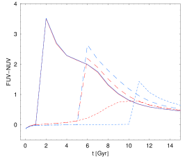
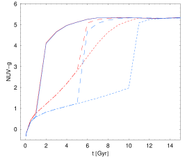
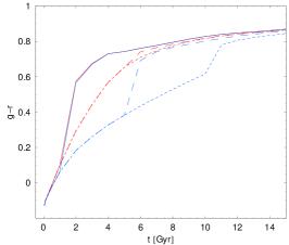
Figure 5: Estimated synthetic colours FUV-NUV, NUV-g and g-r (in AB system) as a function of galaxy age (in units of $\rm Gyr$) for $Z=\mbox{$Z_{\odot}$}$ and for $\tau=1\,\rm Gyr$ (red lines) and $\tau=3\,\rm Gyr$ (blue lines). Continuous, long-dashed and short-dashed lines correspond to $\mbox{$t_{AGN}$}=1,\,5,\,10\,\rm Gyr$.

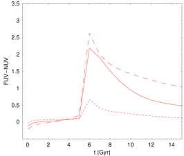
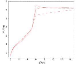
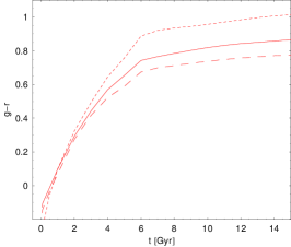
Figure 6: Estimated synthetic colours FUV-NUV, NUV-g and g-r (in AB system) as a function of galaxy age (in units of $\rm Gyr$) for $\tau=1\,\rm Gyr$ and $\mbox{$t_{AGN}$}=5\,\rm Gyr$. Long-dashed, continuous and short-dashed lines correspond respectively to $Z=0.008,\,0.02,\,0.05$.

3.2 Time-scales

Although we discuss the output of only one single simulation, the general model of jet propagation in the ISM which is also probed by our simulation allows us to determine one of the most relevant parameters of the star feedback model that we will develop in the next paragraphs: the typical time-scale for suppression of stellar formation.

In the self-similar expansion model of Kaiser & Alexander (1997), the cocoon is supposed to propagate into an unperturbed ISM which is well described by a power-law profile: $\rho(r)=\rho_{0}(r/a_{0})^{-\beta}$, and the typical scale length of the jet varies with time according to:

$$L_{j}=c_{1}a_{0}\left(\frac{t}{t_{0}}\right)^{3/5-\beta}$$ (3)

where (Kaiser & Alexander 1997, Eq. 5):

$$t_{0}=1.186\times 10^{6}\left(\frac{a_{0}^{5}\,\rho_{0}}{P_{j,45}}\right)^{1/3}\,{\rm yrs.}$$ (4)

and $P_{j,45}$ is the jet’s mechanical power in units of $10^{45}\,\rm erg\,s^{-1}$.
We have assumed that the number density of cold, star-forming clouds is proportional to that of the diffuse gas, and thus can be well approximated by the same power-law density profile outside the core ($r>a_{0}$). There exists a threshold cloud number density under which SF becomes negligible, and we will suppose that this corresponds to a value of the gas density $\rho_{cr}\approx 10^{-27}{\rm g\,cm}^{-3}$, which is reached at a distance: $r_{cr}=a_{0}(\rho_{0}/\rho_{cr})^{1/\beta}$. Inserting this into Eq. (3), we find that the characteristic timescale needed to reach this distance is given by:

$$t_{fb}=t_{0}\left(\frac{\rho_{0}}{\rho_{cr}}\right)^{\frac{5}{\beta(3-\beta)}}c_{1}^{-\frac{5}{3-5\beta}}$$ (5)

We plot in Fig. 3 the dependence of $t_{fb}$ on jet’s power $P_{j}$. As we can see, typical values for the time-scale of feedback are in the range $10^{6}-10^{8}$ yrs, for reasonable values of the input parameters. The values of $P_{j}$ that we choose are representative of the observed mass range of BHs at the centers of typical galaxies, according to the empirical relation between $M_{bh}$ and $P_{j}$ found by Liu, Jiang, & Gu (2006). Thus, the quenching time-scale for our simulation, of the order of a few Myrs, will increase of about two orders of magnitudes for less powerful jets.

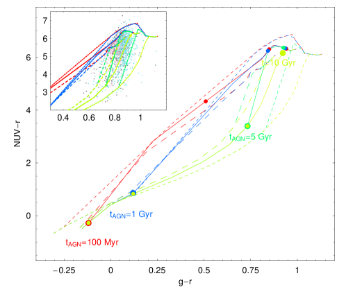
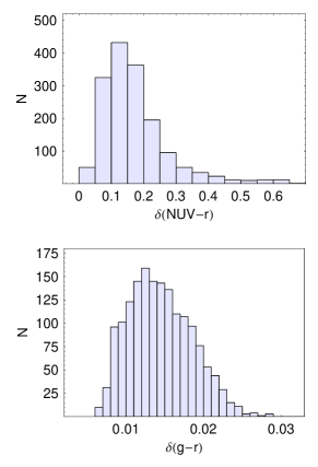
Figure 7: UV/optical colour-colour diagram (NUV-r vs g-r) from synthetic spectra redshifted to median redshift of the sample $z_{med}=0.057$ assuming $\tau=1\,\rm Gyr$ and metallicities $Z=0.008$ (long-dashed line), $Z=0.02$ (continuous line) and $Z=0.05$ (short-dashed line). Red, blue, green and yellow lines correspond, respectively, to $\mbox{$t_{AGN}$}=0.1,\,1,\,5,\,10\,\rm Gyr$. The large points set the values of $t_{AGN}$ on each synthetic track, while the small ones indicate $t_{gal}$ ($=0.1,\,1,\,5,\,10\,\rm Gyr$), which on different tracks correspond to different set of colours after the quenching. In the inset panel we superimpose the sample galaxies to theoretical tracks, with violet, gray and cyan points indicating galaxies in the redshift bins 0–0.04, 0.04–0.06 and 0.06–0.08. Instead of error bars, we show in the right panels the distributions of uncertainties on galaxy colours $g-r$ and $NUV-r$.

4 Synthetic colours

The simulation discussed in this paper describes the impact that the jet emitted by AGN has on quenching SF. However, we would like to transpose this modification of the SF into a change of some observable quantities. Colors and absorption/emission lines are the most important observables given by the observations: here we will concentrate on the former ones. In order to reproduce galaxy colours, we use the synthetic models of Bruzual & Charlot (2003, hereafter BC03), that allows us to encompass a wide range of metallicities, starting from galaxy ages $t_{gal}$ of $10^{5}\,\rm yrs$, and gives a full coverage in wavelength from $91\,\rm{\AA}$ to $160\rm\,\mu m$. We start from a single initial burst model, consisting of a single population with a Chabrier IMF and three values of the metallicities: $Z=0.008,\,0.02$ i.e. ($Z=\mbox{$Z_{\odot}$}$), $0.05$ and convolve it with a SFR law.

We suppose that without interaction of the AGN with the ISM, SF within the clouds evolves following an exponential SF law $SFR\propto e^{-t/\tau}$, where $\tau$ is a characteristic timescale corresponding to the time when SF is reduced of $e^{-1}$.. Then at $t=\mbox{$t_{AGN}$}$, the AGN interaction begins to work, shocking the ISM and inhibiting SF. This configuration can be realized by combining the unperturbed exponential SFR for $t\leq\mbox{$t_{AGN}$}$ and SFR from our simulation for $t>\mbox{$t_{AGN}$}$. Due to the short time-scale involved in the AGN effect on SFR, positive feedback is not observable in the derived colours, while the negative feedback is directly translated into a strong truncation of SFR. Note that this model is an approximation, since less powerful AGNs are observed at low redshifts and the decrease of SF can be shallower, as discussed in the previous section (see, also, the parametric model of SF quenching discussed in Martin et al. (2007a)). If $\tau\to\infty$, the SFR becomes a burst with finite length $t_{AGN}$ (i.e. a SF constant up to $t_{AGN}$ with a null value for $t>\mbox{$t_{AGN}$}$).

We calculate colours by convolving the filter responses of $\rm u,\,g,\,r,\,i$ and z SDSS and the ultraviolet FUV and NUV GALEX bands (Martin et al. 2005, Yi et al. 2005, Kaviraj et al. 2007a) with synthetic spectra. In Figs. 4, 5 and 6 we show the change with time of colours $FUV-NUV$, $NUV-g$ and $g-r$ and the effect of quenching. In particular, in Fig. 4 we compare the colours of our inhibited SF (with $\mbox{$t_{AGN}$}=1$ and $5\,\rm Gyr$) and two simple models using an exponential SF with $\tau=0$ and $\tau=1\,\rm Gyr$. SF inhibition essentially reddens the colours starting at t$>$$t_{AGN}$. Ultraviolet is much sensitive to SF inhibition (see the middle panel in Fig. 4), with variations of $1-3$ magnitudes in $NUV-g$; less sensitive are the visible colours, with variations of $\sim 0.2-0.4$ in $g-r$. The colour FUV-NUV increases after the action of the AGN up to $\sim 1-4$, depending on $t_{AGN}$, but after this event it decreases reaching a value $\mathrel{\hbox to0.0pt{\lower 3.5pt\hbox{\hskip 0.5pt$\sim$}\hss}\raise 0.5pt\hbox{$<$}}1$ for large $t_{gal}$. Therefore, the latter colour is degenerate, because one is not able to univocally determine the galaxy age from colour (each colour corresponds to two possible values of $t_{gal}$).

A single burst model ($\tau=0$) is similar to our models with inhibited SF for $t>2-4\,\rm Gyr$, but predicts larger values for $t<2-4\,\rm Gyr$. While $g-r$ colours for the different models shown in Fig. 4 are similar since $t\sim 6-8\,\rm Gyr$, the other colours are comparable at larger ages $t\sim 8-10\,$ Gyr, being more sensitive to SF. Not shown in the figure is the case $\tau\to\infty$, characterized for fixed values of $t_{AGN}$ and $t_{gal}$  by bluer colours.

These considerations are obviously dependent on the choice of $\tau$ and $Z$. In Fig. 5, we compare the results for $\tau=1$ and $3\,\rm Gyr$. At fixed age, a more protracted unperturbed SF predicts smaller $NUV-g$ and $g-r$ and a larger $FUV-NUV$. Metallicity has the opposite effect: $FUV-NUV$ decreases if we increase metallicity, while g-r increases; finally, a more complex behaviour is observed for $NUV-g$, as can be seen by inspecting Fig. 6. These complex dependencies on metallicity are linked to the details of stellar population prescriptions.

We can outline a picture where the AGN effect has a main role in the evolution of brighter elliptical galaxies. In particular, inhibition of SF by AGN transforms a galaxy with a protracted SF (in our case an unperturbed SF obtained using an exponential SF law with a specific $\tau$) into a more quiescent galaxy with SF stopped at a time approximately equal to the epoch of jet injection. The extreme case of this model is represented by a single burst model, where only at $t=0$ is the SF observable and most of the SF has been completed by this epoch.

5 Epoch of quenching event

We will now attempt to fit synthetic models to a large sample of local ETGs, in order to obtain information about the epoch of quenching event and RSF. The galaxy sample is presented in Sect. 5.1, while the spectral fit procedure and the first results are described in Sect. 5.2. We go into more detail in Sects. 5.3 and 5.4, where quenching and the properties of the recemtly formed stellar populations are discussed. Finally, few comments on galaxy evolution are addressed in Sect. 5.5.

5.1 Galaxy sample

We use a sample of ETGs extracted from the SDSS, using a selection procedure described in Kaviraj et al. (2007a). The initial selection is made using the fracDev parameter in SDSS, that attributes a weight to the best composite (deVaucouleur’s + exponential) fit to the galaxy image in a particular band. The criterion fracDev $>0.95$ has been proven to be extremely robust, allowing one to pick up $\sim 90\%$ of ETGs in a typical sample of SDSS galaxies. Furthermore, a visual inspection of SDSS images is needed to refine the selection: the ability to classify galaxies obviously depends on redshift and apparent magnitude of the observed galaxies. In order to construct a magnitude-limited sample, we restrict ourselves to r-band magnitude $<16.8$ and redshift $z<0.08$. Finally, cross-matching with ultraviolet GALEX data produces the final sample, with measured magnitudes in SDSS bands u, g, r, i, z and GALEX FUV and NUV (see Kaviraj et al. (2007a) for further details). In this way, we have a wide coverage of galaxy spectra, since in the optimal cases, magnitudes in 7 bands are observed, ranging from $\lambda\sim 1500\,\rm\AA$ up to $\lambda\sim 9000\,\rm\AA$. SDSS magnitudes have typical uncertainties of $\sim 0.01$, while GALEX data are more uncertain with mean errors of $\sim 0.25$ and $\sim 0.15$, respectively for FUV and NUV magnitudes.

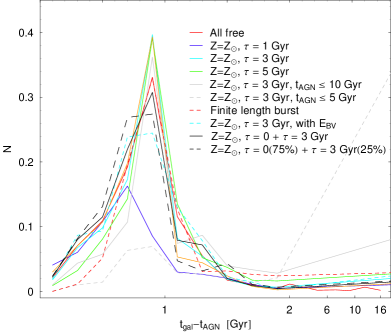
Figure 8: Distribution of recovered best fit values of $\mbox{$t_{gal}$}-\mbox{$t_{AGN}$}$ for different spectra sub-libraries extracted from our initial library. On the y-axis, we plot the fraction of galaxies (normalized to dimension of the sample) within bins of $\mbox{$t_{gal}$}-\mbox{$t_{AGN}$}$. In the range $\mbox{$t_{gal}$}-\mbox{$t_{AGN}$}\in[0-2]\,\rm Gyr$ the scale is linear, while for $\mbox{$t_{gal}$}-\mbox{$t_{AGN}$}>2\,\rm Gyr$ we use an arbitrary logarithmic scale. In the linear range we group galaxies in bins of size $0.2\,\rm Gyr$, while larger bins are used outside this range. In particular, we show the results leaving all parameters free to change, setting $Z=\mbox{$Z_{\odot}$}$ and $\tau=1$, $3$ or $5\,\rm Gyr$, for $\tau=3\,\rm Gyr$ we analyze two cases with constraints on $t_{AGN}$ and then include internal extinction in the fit. We analyze the case of a finite length burst ($\tau=\infty$) and a combination of two coeval stellar populations with $\tau=0$ and $\tau=3\,\rm Gyr$ with a free mass ratio or a fixed one. See labels in the plot and discussion in the text for further details.

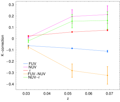
Figure 9: Median K-corrections derived by fitted synthetic spectra for bands FUV, NUV, r and colour FUV-NUV and NUV-r. The bars are the median scatters. See legend for details on the colour code.

In Fig. 7 we show a colour-colour ($NUV-r$ vs $g-r$) diagram from our synthetic tracks. In the inner plot we present our sample, superimposing the galaxies, colour coded according to redshift bins. This diagram gives information about both $t_{gal}$ and $t_{AGN}$  selecting specific values for two colours and the best parameters of galaxies. Different values of galaxy parameters predict galaxy colours that populate different regions of the diagram.

The sample of Kaviraj et al. (2007a) is suitable for our analysis, since AGN spectral features are observed in spectra of many galaxies. Type-I AGN are automatically removed by using the SDSS spectral classification algorithm, while we are interested in galaxies that host a Type-II AGN. To distinguish between normal star forming galaxies and galaxies hosting an AGN, it is usual to analyze a few strong emission lines, e.g. the emission line ratios $[OIII/H\beta]$ and $[NII/H\alpha]$ (1981, Kauffmann et al. 2003). Galaxies with both these indicators measured represent $\sim 65\%$ of the galaxy sample, and $\sim 86\%$ of them have spectral features consistent with those of LINER, Seyfert or transition objects.

Emission from Type-II AGN does not affect the stellar continuum of host galaxies. In fact, for luminous Type-II AGNs the maximum contamination in flux amounts to few percents in visible bands and to less than $15\%$ (translating to 0.15 mags) in UV bands (Kauffmann et al. 2003, Salim et al. 2007). In addition, galaxies hosting AGN are systematically redder in the UV colours than their counterparts which do not have AGNs, further on suggesting that continuum emission from AGN leaves unaffected galaxy spectra.

5.2 Spectral fit

We build a library of synthetic spectra, using our SFR prescription with galaxy age $t_{gal}$, $\tau$, $t_{AGN}$ and $Z$ as free parameters. We divide the sample into 3 redshift bins 0–0.04, 0.04–0.06 and 0.06–0.08 and we move our spectra to the median redshift of each bin (respectively of 0.031, 0.052, 0.069). Synthetic magnitudes and colours are obtained convolving these redshifted spectra with the filter responses. Finally, the synthetic colours are fitted to the observed ones ($FUV-NUV$, $NUV-g$, $u-g$, $g-r$, $g-i$ and $g-z$), by a maximum likelihood method, which allows us to estimate the best values for the free galaxy parameters. In this way we do not need to have K-corrections, leaving the fit safe from possible uncertainties introduced by these corrections, and the simplistic division of our sample into only 3 redshift bins will not affect our estimates. Later, we will discuss the K-correction that we derive from the fitting procedure and we will use to obtain rest-frame magnitudes.

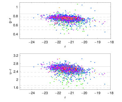
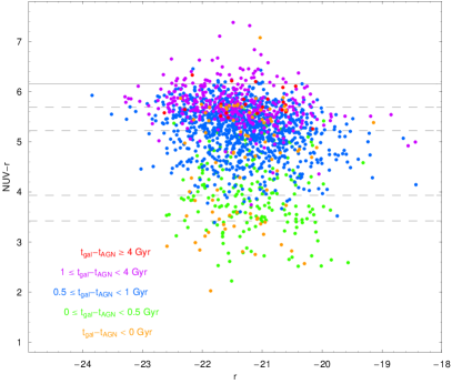
Figure 10: Colour-magnitude diagrams of our sample, colour-coded following the classification shown in the legend: $\mbox{$t_{gal}$}-\mbox{$t_{AGN}$}<0$ (orange), $0\leq\mbox{$t_{gal}$}-\mbox{$t_{AGN}$}<0.5$ (green), $0.5\leq\mbox{$t_{gal}$}-\mbox{$t_{AGN}$}<1$ (blue), $1\leq\mbox{$t_{gal}$}-\mbox{$t_{AGN}$}<4$ (violet), $4\leq\mbox{$t_{gal}$}-\mbox{$t_{AGN}$}$ (red). We show $z=0$ colours predicted using a $z_{f}=3$ single burst population for $Z=\mbox{$Z_{\odot}$}$ as a continuous gray line and various $Z<\mbox{$Z_{\odot}$}$ (i.e. $Z=0.0001,\,0.0004,\,0.004,\,0.008$) as dashed gray lines. Left Panels. We plot g-r vs r and u-r vs r diagrams. Right Panel. We plot NUV-r vs r magnitude.

We restrict synthetic library to spectra with $t_{gal}$ free to change (with a tiny step) up to $17\,\rm Gyr$, $\mbox{$t_{AGN}$}\in(0,15)\,\rm Gyr$, $Z\in(0.008,\,0.02,\,0.05)$ and 3 reference values for the SFR scale $\tau=1,\,3,\,5\,\rm Gyr$. For each value of $t_{gal}$ we have more than 150 spectral models. This library is wide enough to reproduce spectral features of ETGs (2008). The range of metallicities used here has been shown to be representative of luminous ETGs with $M_{B}\mathrel{\hbox to0.0pt{\lower 3.5pt\hbox{\hskip 0.5pt$\sim$}\hss}\raise 0.5pt\hbox{$<$}}-19$ (Romeo et al. 2008, Tortora et al. 2009). In particular, the fit of spectra with an unperturbed exponential SF and variable $Z$ to local ETGs gives on average values of $\tau\mathrel{\hbox to0.0pt{\lower 3.5pt\hbox{\hskip 0.5pt$\sim$}\hss}\raise 0.5pt\hbox{$<$}}1$ and $Z\geq Z_{\odot}$ (Tortora et al. 2009). Such an unperturbed exponential SF with a low time-scale $\tau$ can disguise a more complex SF evolution, which we have obtained from the simulation and want to probe against observations.

Before proceeding to model the properties of the observed sample of galaxies, we briefly discuss the possible systematics which the fitting procedure can generate in the best fitted parameters, by performing a set of Montecarlo simulations on synthetic colours. We have extracted a large sample of simulated spectra from our SED library with random $t_{gal}$, $t_{AGN}$, $\tau$ and $Z$. Then, we applied our fitting procedure and compared the recovered best fit parameters against the intrinsic ones. While $t_{gal}$, $t_{AGN}$ and $Z$ are recovered quite well, $\tau$ is poorly constrained. To reduce the unavoidable degeneracies in the fitting procedure, it would be acceptable to set $\tau$ to a fixed value, however, in the following we will discuss both the cases with $\tau$ variable and constant. In addition, to further reduce the noise in our final results we also analyze the effect of adopting constant metallicity.

Coming back to the observed sample of galaxies, we use different synthetic libraries to fit the observed colours, extracting spectra from our initial and extended set of synthetic models. We show the results of this analysis in Fig. 8, where we plot the distribution of recovered values of $\mbox{$t_{gal}$}-\mbox{$t_{AGN}$}$. If on one hand the change of spectral library can modify the estimates of single values of the parameters, on the other hand it leaves the main clump of the distribution of differences $\mbox{$t_{gal}$}\ -\mbox{$t_{AGN}$}$ unaffected. Due to the correlations among parameters and constraints imposed on some of them, the sample distributions of recovered values for $t_{gal}$, $t_{AGN}$ and Z can change, but median values for $\mbox{$t_{gal}$}\ -\mbox{$t_{AGN}$}$ ($\sim 0.8-0.9\,\rm Gyr$ with a median scatter of $\sim 0.1-0.2\,\rm Gyr$) are almost unchanged, with a scatter among the different estimates consistent with 0. If we impose strong constraints on $t_{AGN}$ (e.g., $\mbox{$t_{AGN}$}\ \leq 5\,\rm Gyr$), we observe a departure from the mean trend obtained using other libraries, with a peak at very large values of $\mbox{$t_{gal}$}-\mbox{$t_{AGN}$}$ (corresponding to quenching at high redshift), but this constraint does not seem to be motivated since it decreases the quality of fit. In addition, note that for $\tau=1\,\rm Gyr$ the distribution peak is slightly lower and less prominent, mainly due to the larger number of galaxies estimated to have unperturbed SF (i.e., with $\mbox{$t_{gal}$}<\mbox{$t_{AGN}$}$). To perform a more complete analysis, we also show the results for a combined spectral model obtained by summing up two coeval stellar populations: a single burst model to a quenched SF assuming a variable or a fixed mass ratio of the two populations. This model takes into account the coexistence of stellar populations having different properties: a part of stars formed in a single initial burst, in addition to this component, there is gas which cools to form continuously stars and is affected by AGN. What we see in Fig. 8 is that these combined models we have discussed give the same results as using the single component ones. Our estimates of $\mbox{$t_{gal}$}-\mbox{$t_{AGN}$}$ are robust, since the bulk of their distribution depends little on the duration of the unperturbed SF and $Z$. Despite this result, as we will see later, the past SF history of galaxies is dependent on the choice of these models. Finally, two shortcomings have to be discussed. If considering more protracted unperturbed SF we will obtain a larger number of galaxies with higher $\mbox{$t_{gal}$}-\mbox{$t_{AGN}$}$ values than using SFs with lower $\tau$ (see Fig. 8). In addition, a similar effect is given if quenching is not almost instantaneous as in our simulation, also in this case we would obtain larger values of $\mbox{$t_{gal}$}-\mbox{$t_{AGN}$}$. However, our fast quenching is a good approximation to describe AGN effect for a wide sample of galaxies, but further analysis on these aspects waits to be done in future.

In order to avoid confusion, we will use in the following the results obtained in the most general case where $Z$, $\tau$, $t_{gal}$ and $t_{AGN}$  are all unconstrained. Also, K-corrections deserve particular attention. In fact, due to uncertainties in the UV spectrum, it can be difficult to quantify the amount of this correction, acircumstance which can introduce systematics. In our range of redshifts, we find typical NUV corrections of $0-0.3$, in good agreement with those found in Kaviraj et al. (2007a) using the same galaxy catalog. In Fig. 9, we show also results for K-corrections of FUV, r and colours FUV-NUV and NUV-r. We obtain a sharp rise in NUV correction: this is negligible in the lowest redshift bin, while its median value becomes $\sim 0.25$ at higher z. The median scatter in the estimated values of NUV and FUV corrections is consistent with typical uncertainties of observed magnitudes in these bands. Note that Kaviraj et al. (2007a), using a $9\,\rm Gyr$ old single burst model and Rawle et al. (2008), using both single burst and frosting models, find larger corrections of $0.2-1.2$ for galaxies having $z\mathrel{\hbox to0.0pt{\lower 3.5pt\hbox{\hskip 0.5pt$\sim$}\hss}\raise 0.5pt\hbox{$<$}}\,0.1$.

5.3 Quenching event

In Fig. 10 we show the visible and UV colour-magnitude diagrams for our sample. As already detailed in Kaviraj et al. (2007a), the UV diagram in the right panel of this figure is largely different from similar colour diagrams for optical bands (see left panels), since it shows a larger scatter. Fig. 10 shows the power of $NUV-r$ colour in selecting galaxies with different SFR histories. In particular, the points in the figure are colour-coded according to the fitted value of $\mbox{$t_{gal}$}-\mbox{$t_{AGN}$}$: galaxies that experienced some quenching phenomena in the past lie upper in this diagram, while those having lower values of this quantity populate on average a region with a flatter UV continuum and a larger scatter.

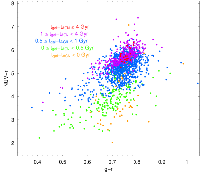
Figure 11: UV/optical colour-colour diagram. We plot NUV-r vs g-r of galaxies in our sample colour-coded following the classification shown in the legend.

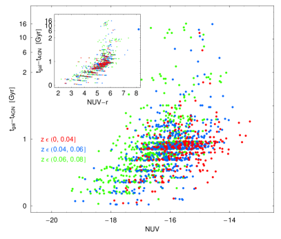
Figure 12: $\mbox{$t_{gal}$}-\mbox{$t_{AGN}$}$ as a function of ultraviolet magnitude NUV, while in the inserted panel is plotted $\mbox{$t_{gal}$}-\mbox{$t_{AGN}$}$ as a function of colour NUV-r. Points are colour coded for various redshift bins. See Fig. 8 for details on the scale used in the y-axes.

A rough comparison with the expectation of the monolithic scenario has been made, superimposing the predicted colours for single burst populations with a more extended formation redshift starting at $z_{f}=3$. For completeness, in addition to a model with $Z=\mbox{$Z_{\odot}$}$ we also show the predictions for various metallicities $<\mbox{$Z_{\odot}$}$ implemented within BC03 prescription. These predictions are not very sensitive to the precise value of $z_{f}$ (at least when considering relatively old stellar populations), and our choice is consistent with optical analyses which estimate $z_{f}~{}\hbox to0.0pt{$>$\hss}{\lower 4.30554pt\hbox{$\sim$}}\,2$ (Bower et al. 1992). We see that an almost solar single burst model is only consistent with redder galaxies both for g-r and NUV-r colours. Thus, while galaxies with low g-r and NUV-r can be matched by models with low $Z$, galaxies in the u-r vs r plot appear to depart from these predictions which systematically lead to redder colours. However, as we pointed out in a previous subsection, luminous ETGs are almost solar and very low values of metallicities like those used in Fig. 10 are not applicable to our galaxies (2008, Tortora et al. 2009). Moreover, semi-analytic simulations predict that a single solar metallicity is a reasonable hypothesis to describe ETGs (Nagashima & Okamoto 2006) and similar results for the brighter and more massive galaxies have been obtained in N-body+hydrodynamical simulations (Romeo et al. 2008). Thus, the comparison with a solar metallicity single burst model indicates that only a few galaxies ($\mathrel{\hbox to0.0pt{\lower 3.5pt\hbox{\hskip 0.5pt$\sim$}\hss}\raise 0.5pt\hbox{$<$}}\,6-7\%$) are consistent (within the errors) with a single and old stellar population; these galaxies are the redder ones mainly with $\mbox{$t_{gal}$}-\mbox{$t_{AGN}$}~{}\hbox to0.0pt{$>$\hss}{\lower 4.30554pt\hbox{$\sim$}}\,1$. This result is consistent with the $\mathrel{\hbox to0.0pt{\lower 3.5pt\hbox{\hskip 0.5pt$\sim$}\hss}\raise 0.5pt\hbox{$<$}}\,1\%$ of purely passive galaxies found in Kaviraj et al. (2008) analyzing a sample of galaxies at $z~{}\hbox to0.0pt{$>$\hss}{\lower 4.30554pt\hbox{$\sim$}}\,0.5$, since in the local universe we observe a larger number of quiescent and passive galaxies.

In Fig. 11 we show NUV-r vs g-r, with points colour-coded according to Fig. 10. A correlation is observed, but note that the excursion in NUV-r is much larger than in g-r.

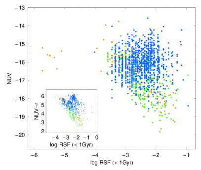
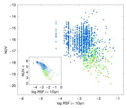
Figure 13: NUV (and NUV-r) vs. RSF for a model leaving free all parameters (left panel) and one with $Z=\mbox{$Z_{\odot}$}$ and $\tau=3\,\rm Gyr$ (right panel). The colour code is the same as in Figs. 10 and 11.

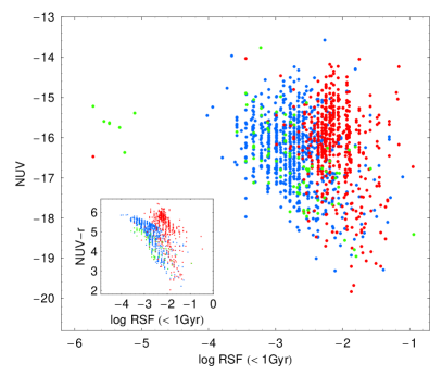
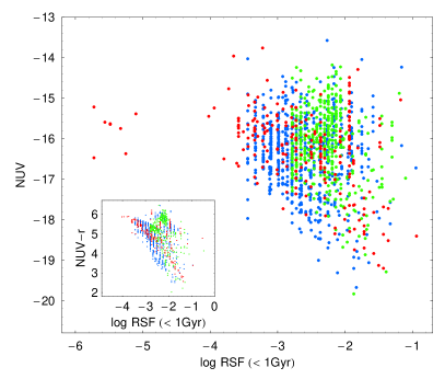
Figure 14: NUV (and NUV-r) vs RSF for a model leaving free all parameters. In the left panel we colour for Z, with $Z=0.008$ (green), $Z=0.02$ (blue) and $Z=0.05$ (red). In the right panel we colour for $\tau$ with $\tau=1\,\rm Gyr$ (red), $\tau=3\,\rm Gyr$ (blue) and $\tau=5\,\rm Gyr$ (green).

Galaxies with a stronger ultraviolet flux are on average characterized by higher RSF, that translates into lower values of $\mbox{$t_{gal}$}-\mbox{$t_{AGN}$}$, while those with a lower NUV flux have SF that is quenched early. This correlation is shown in Fig. 12. In the inner panel, we show the trend with colour NUV-r, implicit in Fig. 10.

The results concerning the scale of SF are also interesting. When considering the results obtained fitting our reference spectral library, we find that only $\sim 15\%$ of galaxies have $\tau=1\,\rm Gyr$, while a more protracted SF is recovered for the other galaxies in the sample, with $\sim 43\%$ and $\sim 42\%$ of these having $\tau=3$ and $5\,\rm Gyr$. As a comparison, we also fitted unperturbed SFs with $\tau\in(0.1,\,5)\,\rm Gyr$ and $Z\in(0.008,\,0.02,\,0.05)$ obtaining that $\sim 86\%$ of galaxies have $\tau\leq 1$, while less than $1\%$ have $\tau>3\,\rm Gyr$ (see also Tortora et al. 2009). Thus, the low SF scales recovered when simple unperturbed exponential SFs are fitted to data can hide a galaxy population with a more protracted background SF that is quenched in the late stage of galaxy evolution for a feedback effect. These results are consistent with the general scenario depicted for the color evolution of E+A galaxies in Kaviraj et al. (2007b). They find that, superimposed to an early burst of formation, a recent SF burst (which typically takes place within $1\,\rm Gyr$) over a timescale ranging between 0.01 and 0.2 Gyrs is needed to match galaxy colours. These galaxies are just migrating towards the red sequence and show a SF quenching which is correlated with their stellar mass and velocity dispersion and linked to different sources of feedback (AGN or supernovae). However, although also different models can have the same final result as our unperturbed and truncated SFs for different class of galaxies, this work reproduces typical timescales consistent with those discussed here (see also Fig. 3).

Fitting our reference library, we find that $\sim 35\%$ of galaxies have $\mbox{$t_{gal}$}>t_{Univ}$, while this percentage decreases to $\sim 15\%$ for those galaxies with $\mbox{$t_{gal}$}>t_{Univ}+2$. Excluding all galaxies with $\mbox{$t_{gal}$}>t_{Univ}$ we find a median formation redshift of $z_{f}=1.0^{+1.4}_{-0.4}$ (uncertainties are $25^{\rm th}$ and $75^{\rm th}$ percentiles); note that the distribution has a strong tail for high formation redshift. For $t_{AGN}$ we find the best estimate $z_{AGN}=0.13\pm 0.02$.

5.4 Stellar mass fraction and AGN feedback

Until now, we have discussed how the quenching event is linked to colours and galaxy luminosities, but we have not expressly discussed the amount of stellar mass that is produced. To quantify this recent star formation, we define the RSF via the amount of stars produced (i.e. the produced stellar mass fraction) in the last $1\,\rm Gyr$ in the rest frame of the galaxy (Kaviraj et al. 2007a, 2008). As discussed in the previous subsections, this quantity is strictly dependent on the time of the quenching event, and in particular on $\mbox{$t_{gal}$}-\mbox{$t_{AGN}$}$. The latter has been show to depend on colour NUV-r and the luminosity in the NUV band, while it is less sensitive to the same quantities obtained only using visible bands.

Galaxies with brighter ultraviolet fluxes and bluer NUV-r colours have much more RSF with respect to fainter ones. This result is not surprising, since an indication of it has been obtained by the trends shown in Fig. 12. In Fig. 13 we show the RSF as a function of NUV and NUV-r. In the left panel, we show the results using our reference library. Obviously, only galaxies with $\mbox{$t_{gal}$}-\mbox{$t_{AGN}$}$ less than $1\,\rm Gyr$ survive in these plots and show the presence of RSF. In this case, the trends are not so tight, since some galaxies depart from them (red points). As a comparison, in the right panel we show the results for a model with fixed values of $Z$ and $\tau$, where the correlations are tighter. Coming back to the results we obtained using our reference library, we show in Fig. 14 the same results already plotted in the left panel of Fig. 13, but now coded for metallicity and $\tau$, respectively in the left and right panels. These plots show that those galaxies, which experience a significant RSF, also have metallicities significant different from the average. In fact, galaxies with different metallicities seem to stay on three different sequences, with a lot of supersolar galaxies having red colours and a low NUV flux, but a large SF. This trend is more evident if we look at the plot as a function of colour. The trends with SF time-scale $\tau$ are less clear, but some of those galaxies departing from the mean trend have $\tau=5\,\rm Gyr$. Thus, some systematics might be introduced into these results by the degeneracies between $Z$ and $\tau$, and possibly with other parameters. However, our results are robust, since qualitatively we recover some trends which do not depend on the particular choice of spectral library.

For the model that leaves all of the parameters free, we find a median RSF of $\sim 0.2^{+0.4}_{-0.2}\%$. In particular, galaxies with the bluest colours (and with larger NUV fluxes) have RSF of $\sim 1\%$, while the redder ones have RSF less than $0.1\%$. On the contrary, a lower median RSF of $\sim 0.1\%$ is observed for the model with $\tau=3\,\rm Gyr$ and $Z=\mbox{$Z_{\odot}$}$.

On average, our recovered RSF fractions are slightly lower than those obtained in Kaviraj et al. (2007a), but this is not surprising since we follow a different approach. In detail, we adopt what we can call a blue-to-red approach, since we have modelled galaxies using an exponential SF. Thus, a galaxy is initially blue, and later it becomes red since SF is quenched. On the contrary, using a red-to-blue approach, galaxies are modelled with a single burst population, which predict systematically redder colours than those obtained with a more complex SF. Thus, to match the observations one needs a recent burst to make the colours bluer. It is however worth to be noted that within scatter the two analysis give fully compatible results.

Our results can also be connected with the downsizing scenario. In fact, the fact that redder galaxies (i.e. with a lower NUV flux) have less RSF with respect to the bluer ones can reproduce the trends found in recent works (Cowie et al. 1996, Borch et al. 2006, Bundy et al. 2006, De Lucia et al. 2006, Trager 2000, Thomas et al. 2005, 2005, Kaviraj et al. 2008, Romeo et al. 2008, Tortora et al. 2009). However, this connection has to be better analyzed and further information could be recovered by extending the luminosity range.

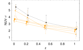
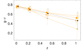
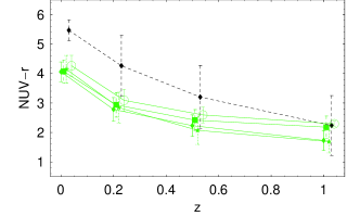
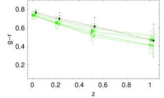
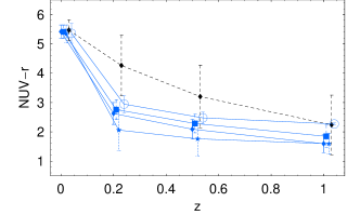
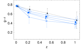
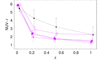
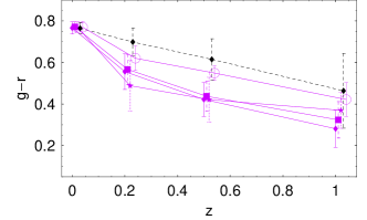
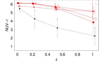
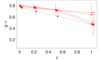
Figure 15: Colour evolution predicted by fit. The different panels refer to values of $\mbox{$t_{gal}$}-\mbox{$t_{AGN}$}$ accordingly to the same colour coding of Figs. 10, 11 and 13. We show the results from our reference model leaving all parameters free to change (star symbols and short-dashed error bars), $Z=\mbox{$Z_{\odot}$}$ and $\tau=3\,\rm Gyr$ (diamond symbols and continuous error bars), two combined models with a $Z=\mbox{$Z_{\odot}$}$ burst superimposed to a truncated exponential SF with $\tau=3\,\rm Gyr$ with a free mass ratio (box symbols and long-dashed error bars) and one with single burst amounting to the $75\%$ of the total mass (circle symbols and thin continuous error bars). The black symbols and bars are obtained using an unperturbed SF with $\tau$ and $Z$ free to change (averaged over all galaxies in the sample). At each redshift, the different models are artificially shifted to make clearer the appearance. Left panels. NUV-r vs z. Right panels. g-r vs z.

5.5 SED evolution

In the previous subsection, we obtained results that indicate the presence of a RSF that is connected with the quenching events. Here, we quantify the evolutive path of galaxies in our sample, discussing how colours and magnitudes (averaged over the galaxy sample) evolve. A more detailed analysis of these results is beyond the scope of this paper.

We verified that a large part of the galaxies in our sample are not very sensitive to changes of the details of the spectral library, since they predict a median $\mbox{$t_{gal}$}-\mbox{$t_{AGN}$}$ that does not change siginficatly (see Fig. 8). Thus, our models are able to successfully describe the recent formation history of galaxies, while the extrapolation to early phases of galaxy evolution is influenced by the choice of unperturbed synthetic spectra. However, this extrapolation can fail to describe the earlier evolution, since galaxies which have experienced various (minor or major) mergers, and AGNs can act to quench SF at different epochs (2008). Therefore, both SF, magnitude and colour evolution can be very complex and is not possible to efficiently probe them.

We map the evolution of rest-frame galaxy colours up to 7-8 billion of years ago, that we determine from our best fitted models for 3 values of the look-back time $t_{lbt}$ corresponding to redshift $z=0.2,\,0.5,\,1$. In Fig. 15 we show the median values and median deviations for $NUV-r$ and $g-r$ of galaxies in the sample. Actually, colour and luminosity evolution is stronger for galaxies with a more recent event of SF and quenching (i.e. lower $\mbox{$t_{gal}$}\ -\mbox{$t_{AGN}$}$). These galaxies became red only recently, while those with a quenching event that occurred many Gyrs ago were already on the red sequence. While changes of 2-3 magnitudes in NUV-r are observed, g-r changes are $\mathrel{\hbox to0.0pt{\lower 3.5pt\hbox{\hskip 0.5pt$\sim$}\hss}\raise 0.5pt\hbox{$<$}}1$ magnitude. In addition to our reference model, we show the evolution of colours obtained using a library of truncated SFs with $Z=\mbox{$Z_{\odot}$}$ and $\tau=3\,\rm Gyr$ and two mixed models consisting of a solar single burst and a truncated SF with $Z=\mbox{$Z_{\odot}$}$ and $\tau=3\,\rm Gyr$, leaving free the proportion of the two populations, and fixing the single burst to 75% of the total mass. These two latter models leave the galaxy colours for $\mbox{$t_{gal}$}>\mbox{$t_{AGN}$}$ almost unchanged, while affecting the early history of galaxies producing redder colours, this effect depending on the ratio of the two populations. For comparison, we show the median colours obtained fitting an unperturbed SF leaving free to change $t_{gal}$, $Z$ and $\tau$.

These predicted tracks show an interesting result concerning the strength of quenching, that is mainly evident in the NUV-r colour. With the exception of galaxies with $\mbox{$t_{gal}$}<\mbox{$t_{AGN}$}$ and those with an early quenching event, the systems with an observed larger colour difference (and thus on average large values of $\mbox{$t_{gal}$}-\mbox{$t_{AGN}$}$) were bluer and more star forming at $z\sim 0.2$. Thus, this result seems to indicate that in galaxies with a large SF at $z~{}\hbox to0.0pt{$>$\hss}{\lower 4.30554pt\hbox{$\sim$}}\,0.2$, the effect of AGN quenching can be stronger, to produce the reddest galaxies we observe today. Nonetheless, recent X-ray and optical selected analysis of high redshift AGNs (Martin et al. 2007b, Nandra et al. 2007, Silverman et al. 2008a, b) exhibit a large fraction of AGN in galaxies at intermediate/blue colours, which could be driven by AGN feedback toward red-sequence at $z\sim 0$.

The magnitudes NUV and r against redshift are plotted in Fig. 16. The estimated evolution of the NUV magnitude, being strongly sensitive to RSF, can be different among models, and is compared to those obtained using an unperturbed SF. The NUV fluxes are systematically larger (corresponding to lower $NUV-r$) than those estimated using unperturbed SFs. On the contrary, the luminosity in the r band does not depend (or at least depends only little) on a change in models and the predictions agree quite well. This is not surprising, since redder bands are less sensitive to recent or past SF.

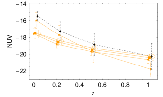
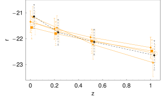
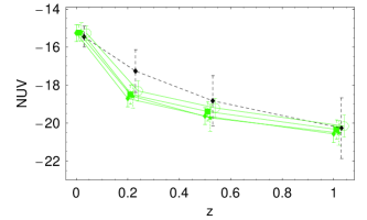
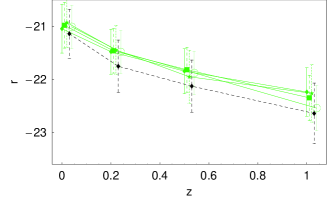
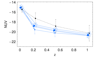
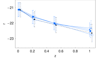
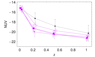
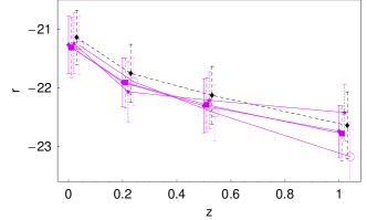
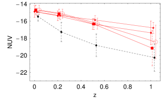
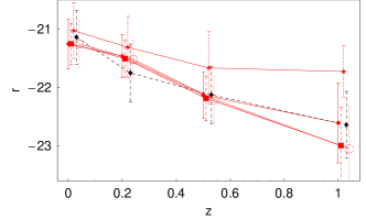
Figure 16: Magnitude evolution predicted by fit. See Fig. 15 for details about models and colour or symbol code. Left panels. NUV vs z. Right panels. r vs z.

6 Conclusions

In this work, we have attempted to build up a realistic model of AGN feedback. We performed a hydrodynamical simulation to analyze the impact of jets produced by AGNs on a inhomogeneous medium, properly representing cold gas clouds that form stars in galaxies. In our simulation, which extends and generalizes a set that we previously performed (Antonuccio-Delogu & Silk 2008), a powerful jet $P_{j}=10^{46}\,\rm erg\,s^{-1}$ propagates within an inhomogeneous, two-phase ISM, containing a realistic distribution of star-forming clouds. SFRs in clouds are described using the empirical SK prescription, where the SFR depends on the mass density of the star forming regions of the clouds. In an early phase, the shocks advancing before the expanding cocoon tend to compress the cold clouds, without significantly changing the temperature of the medium, thus increasing the SF. Later, when the cocoon has propagated within the medium, the temperature of both the medium and of the clouds increases significantly and the mass of clouds is reduced, also due to KH instabilities. Thus, at the beginning, a positive feedback increases SF, but the dominant effect is the negative feedback that quenches SF in a time of $\sim 2-3\times 10^{6}\,\rm yr$. One interesting result of this paper is that for the first time a hydrodynamical simulation allows the determination of the effect of jets emitted by AGN on SF in galaxies. Previous work has insted relied relying on empirical prescriptions to take into account AGN feedback (Granato et al. 2001, 2004, Cattaneo et al. 2006, Martin et al. 2007a), and are thus more robustly supported by our results.

The high jet power in this simulation is probably the main reason of the fact that, at the end of the simulation, all the gas within the computational volume is in a physical state for which all SF is quenched. For lower injection powers, the cocoon expansion will be halted before, and the region where SF is quenched will consequently be smaller.

Based on the results of this simulation, we develop a more general model which assumes a SFR for ETGs composed of a background SF with a more or less extended duration, that is quenched by a feedback effect such as that analyzed in the first part of this paper. However, we stress here that this general prescription can also describe the effect of other quenching mechanisms, like merging, harassment, etc. Restricting ourselves to the case of a high power jet, as in the present paper, the typical timescales of quenching are very small, and no other sources of feedback can stop SF within such a short time. Note also that galaxy merging seems to be one of the mechanisms which activate AGNs, which after the burst induced by the merger is able to quench the residual SF in the remnant (Di Matteo et al. 2005, 2008).

Our paradigm is that luminous ETGs are an exception within the zoo of galaxies in the universe. We suppose that the normality in galaxy samples is represented by fainter ETGs, that have a protracted SF, but by the effect of feedback they are quenched and colours redden. This could be one of the missing physical ingredients which could explain the short duration of SF, when exponential SF are fitted to data (e.g., Tortora et al. 2009). On the contrary, semi-analytical galaxy simulations predict more protracted SFR (De Lucia et al. 2006): supernovae feedback was taken into account in these simulations, but the disagreement with other observations can be due to an improperly accounted for contribution from AGNs. Springel et al. (2005a) simulate the effect of AGNs in the merging of two massive and gas-rich spiral galaxies, obtaining similar results. They found that SF is inhibited with respect to the case without black holes; interestingly, without AGNs this kind of merger is not able to produce red ETGs, that remain blue (with residual SF) even after several Gyrs. On the contrary, the presence of black holes redden galaxy colours much faster, giving $u-r\sim 2.3$ in less than 1 Gyr after the beginning of the merging process.

We assume an unperturbed SF law with a scale $\tau=1,\,3,\,5\,\rm Gyr$, that is quenched at $t_{AGN}$  leaving free to change these parameters as well as galaxy ages and metallicities. We fit these models to observations from a cross-matched SDSS+GALEX catalog. Confirming the results in Kaviraj et al. (2007a), the UV has been shown to be a strong indicator of SF, in particular, the UV/optical colour $NUV-r$ allows us to select galaxies with different levels of SF, stopped in the last Gyrs or still in action. We show that the quantity $\mbox{$t_{gal}$}-\mbox{$t_{AGN}$}$ is able to describe the physical state of galaxies, indicating how much time ago SF is stopped. The largest number of galaxies have $\mbox{$t_{gal}$}-\mbox{$t_{AGN}$}\sim 0.5-1\,\rm Gyr$, indicating the necessity of a RSF phenomenon (until $1-2\,\rm Gyr$ ago), that is quenched by AGNs. Galaxies with larger $NUV-r$ have higher values of $\mbox{$t_{gal}$}-\mbox{$t_{AGN}$}$, i.e. SF is quenched early in their history, while lower values of $NUV-r$ correspond to galaxies with a more recently quenched SF. Finally, galaxies with a SF not affected by AGN have the flattest $NUV-r$ colours. This distinction is not so clear (or absent) for visible colours. These results are shown in Figs. 10 and 11. The epoch of the quenching event appears to be correlated with ultraviolet flux: galaxies bluer and brighter in NUV band are also those with a more recent (or absent) quenching event. As shown in Fig. 8, $\mbox{$t_{gal}$}-\mbox{$t_{AGN}$}$ is found to negligibly depend on the details of background spectral library (e.g., $\tau$ and $Z$), at least for the bulk of galaxies: thus we obtain a robust estimate of the quenching time and RSF. Our analysis is less sensitive to the earliest phases of galaxy history, notwithstanding the mean evolution of galaxy population here analyzed, as shown in Figs. 15 and 16. Finally, a shortcoming of this analysis is related to the timescale of quenching event, since softer power jets would inhibit SF within a larger timescale. Such a slower quenching model would be fitted to the colours by a larger $\mbox{$t_{gal}$}-\mbox{$t_{AGN}$}$, thus our results for this parameter have to be interpreted as lower limits.

One of the most significant results we have found is that the NUV-g colour index is very sensitive to the presence of a very young stellar population. Typical enhancement of 2-3 magnitudes of NUV-g are observed, with regard to the no-feedback case. Our findings agree with some current simulations that invoke two different modes of AGN feedback. A so called ‘quasar mode’ assumes that during a major merger event at high redshift, a fraction of the gas accreted by a central black hole is injected into the gas of the host galaxy, quenching SF (Springel et al. 2005a, b, Di Matteo et al. 2005). At later times, another effect is important, i.e. the ‘radio mode’, that is responsible for making galaxies quiescent, and this effect is driven by low-level AGNs (Croton et al. 2006, Bower et al. 2006). More recently, Schawinski et al. (2008) speak of a ‘truncation mode’ to indicate AGN feedback at high redshift. At recent epochs, no such strong activities or powerful radio jets have been observed, and so this kind of AGN feedback is often referred to as the ‘suppression mode’. These authors suggest that this process could leave a residual SF (e.g. Schawinski et al. 2006), but is able to move galaxies along the red sequence.

Further refinements of our analysis are needed. Firstly, it is important to enlarge the sample of galaxies and analyze a more extended range of magnitudes. The galaxies under analysis, due to constraints on magnitude, are relatively bright with $M_{B}\mathrel{\hbox to0.0pt{\lower 3.5pt\hbox{\hskip 0.5pt$\sim$}\hss}\raise 0.5pt\hbox{$<$}}-19$. Different kinds of analysis seem to indicate that brighter and more massive ETGs ($M_{B}\mathrel{\hbox to0.0pt{\lower 3.5pt\hbox{\hskip 0.5pt$\sim$}\hss}\raise 0.5pt\hbox{$<$}}-20.5$ and $M_{\star}~{}\hbox to0.0pt{$>$\hss}{\lower 4.30554pt\hbox{$\sim$}}\,10^{11}\,\rm\mbox{$M_{\odot}$}$) are fundamentally different from fainter and less massive ones ($M_{B}~{}\hbox to0.0pt{$>$\hss}{\lower 4.30554pt\hbox{$\sim$}}-20.5$ and $M_{\star}\mathrel{\hbox to0.0pt{\lower 3.5pt\hbox{\hskip 0.5pt$\sim$}\hss}\raise 0.5pt\hbox{$<$}}\,10^{11}\,\rm\mbox{$M_{\odot}$}$). In these two different luminosity and mass regimes, the size-luminosity or size-mass (Shen et al. 2003) and Faber-Jackson relations (Matkovi$\rm\acute{c}$ & Guzm$\rm\acute{a}$n 2005) have different slopes. Also, the Sersic index is changing with luminosity (Prugniel & Simien 1997), and dark matter is shown to have a bivariate behaviour in the two ranges (Tortora et al. 2009), suggesting that physical phenomena allowing the formation of galaxies of different mass and luminosity can be variegate. Thus, a future analysis should also be directed at studying a wider range of luminosities and masses to map the transition from the blue cloud to the red sequence. Also to connect our results with the downsizing scenario, we need to enlarge the sample to fainter magnitudes, since strong changes in observable quantities such as galaxy age, $t_{AGN}$  $\tau$ and $Z$ are probably visible in these luminosity regimes. We are planning to do other simulations changing the main input parameters, in order to have a more reasonable model of AGN feedback which depends, e.g., on the jet power, linking it to main galaxy observables (Liu, Jiang, & Gu 2006). Comparison with simulations will allow to quantify how much AGN feedback has to be implemented, to make both semi-analytical and hydrodynamical simulations able to correctly predict the main properties of galaxies we observe. Such a more complex model of quenching would be parameterized as a function of the main parameters of the system and compared to other AGN feedback prescriptions (Granato et al. 2001, 2004, Cattaneo et al. 2006, Martin et al. 2007a).

Linking observations at low redshift, such as those analyzed here, with high redshift data (Martin et al. 2007b, Nandra et al. 2007, Silverman et al. 2008a, b) could certainly be a powerful way to shed light on the galaxy evolution scenario, and in particular the role that AGNs have in the early and later phases of the SF history of galaxies.

References

- Antonuccio-Delogu & Silk (2008) Antonuccio-Delogu V. & Silk J. 2008, MNRAS , 389, 1750
- Baek et al. (2005) Baek C. H., Kang H., Kim J., & Ryu D. 2005, ApJ , 630, 689
- (3) Baldwin J. A., Phillips M. M. & Terlevich R. 1981, PASP, 93, 5
- Benson et al. (2003) Benson A. J. et al. 2003, ApJ, 599, 38
- Bicknell et al. (1997) Bicknell G. V., Dopita M. A., O’Dea C. P. O. 1997, ApJ, 485, 112B
- Bildfell et al. (2008) Bildfell C., Hoekstra H., Babul, A., Mahdavi, A. 2008, MNRAS, 389, 1637
- Bonnor (1956) Bonnor W. B., 1956, MNRAS , 116, 351
- Borch et al. (2006) Borch A., et al. 2006, A&A 453, 869
- Bower et al. (1992) Bower R. G., Lucey, J.R., Ellis, R. 1992, MNRAS, 254, 589
- Bower et al. (2006) Bower R. G. et al. 2006, MNRAS, 370, 645
- Bruzual & Charlot (2003) Bruzual A. G. & Charlot S. 2003, MNRAS, 344, 1000
- Bundy et al. (2006) Bundy K., et al. 2006, ApJ, 651, 120
- Cattaneo et al. (2006) Cattaneo, A., Dekel, A., Devriendt, J., Guiderdoni, B., & Blaizot, J., 2006, MNRAS, 370, 1651
- Cowie et al. (1996) Cowie L. L., Songaila A., Hu E. M., Cohen J. G. 1996, AJ, 112, 839
- Croton et al. (2006) Croton D. J. et al. 2006, MNRAS, 365, 11
- Dekel & Silk (1986) Dekel A. & Silk J., 1986, ApJ, 303, 39
- De Lucia et al. (2006) De Lucia G., Springel V., White S. D. M., Croton D., Kauffmann G. 2006, MNRAS, 366, 499
- Di Matteo et al. (2005) Di Matteo T., Springel V. & Hernquist L. 2005, Nature, 433, 604
- Ebert (1955) Ebert R., 1955, Zeitschrift fur Astrophysik, 37, 217
- Falle (1991) Falle S. A. E. G., 1991, MNRAS , 250, 581
- Fryxell et al. (2000) Fryxell B., Olson K., Ricker P., Timmes F. X., Zingale M., Lamb D. Q., MacNeice P., Rosner R., Truran J. W., Tufo H., 2000, Astrop. J. Supp. , 131, 273
- Granato et al. (2001) Granato G. L., Silva L., Monaco P., Panuzzo P., Salucci P., De Zotti G., & Danese L. 2001, MNRAS, 324, 757
- Granato et al. (2004) Granato G.L., De Zotti G., Silva L., Bressan A. & Danese L. 2004, ApJ, 600, 580
- Hasinger et al. (2005) Hasinger, G., Miyaji, T., & Schmidt, M. 2005, A& A , 441, 417
- (25) Hester J. A. 2006, ApJ , 647, 910
- (26) Iliev I. T., & Shapiro P. R. 2001, MNRAS , 325, 468
- (27) Inoue S. & Sasaki S., 2001, ApJ , 562, 618