Generation of multi-photon entanglement by propagation and detection

Abstract

We investigate the change of entanglement of photons due to propagation. We find that post-selected entanglement in general varies by propagation and, as a consequence, states with maximum bi- and tri-partite entanglement can be generated from propagation of unentangled photons. We generalize the results to n photons and show that entangled states with permutation symmetry can be generated from propagation of unentangled states. Generation of n-photon GHZ states is discussed as an example of a class of states with the desired symmetry.

I Introduction

It is well-known that the classical coherence properties of an electromagnetic field vary due to propagation Mandel and Wolf (1995). The most well-known example of this is the increase of the spatial coherence of the radiated field from an incoherent source upon propagation van Cittert (1934); Zernike (1938); other examples are the Wolf effect, the variation of the spectrum of light under propagation Wolf (1987); Wolf and James (1996), and the change of polarization of light under propagation James (1994). It is therefore reasonable to pose the question: can propagation alter the quantum correlations of a field? In this paper, we study the change of entanglement on propagation and answer this question in the affirmative. A direct consequence of this result is post-selective generation of polarization-entangled photons through propagation of unentangled photons. For two photons this result has been pointed out by Lim and Beige Lim and Beige (2005) and is similar in spirit to entanglement generation schemes in linear optics Eibl et al. (2003); Fattal et al. (2004); Pan et al. (2001), where erasure of which-path information leads to creation of entanglement. The scheme has also been implemented in reverse to generate entangled atoms by detection of photons Cabrillo et al. (1999); Matsukevich et al. (2008). Here, we extend these considerations to three photons and demonstrate that propagation and post-selective measurement can be used to create states with maximum genuine tri-partite entanglement Coffman et al. (2000). Furthermore, we show that a generalization of this result leads to creation of $n$-photon Greenberger-Horne-Zeilinger (GHZ) states.

Multi-photon entangled states have been generated for up to six photon by down-conversion and linear-optics Lu et al. (2007) and are of interest for optical quantum computing Knill et al. (2001); Kok et al. (2007). Moreover, many-particle entangled states are a resource in the one-way quantum computing paradigm Raussendorf and Briegel (2001); Briegel et al. (2009) which can be implemented advantageously in a linear optics setting Browne and Rudolph (2005); Prevedel et al. (2007); Dev . Interferometric stability and beam-splitter alignment are major obstacles in creation of larger entangled states by linear optics techniques. It would therefore be desirable to create multi-photon entanglement by simpler optical arrangements which may relax the requirement for beam-splitter alignment and stability. The schemes considered in this paper rely solely on free-space propagation and detection; our study offers insight into generation and manipulation of optical entanglement without the need for beam-splitters or non-linear optical elements. One major drawback of the proposed scheme is the exponential scaling with the number of qubits due to the n-photon coincidence count. However, this deficiency can possibly be overcome via classical interference, and is currently under further investigation.

II Two photon case

II.1 Generation of Entanglement

As an example of a simple situation in which propagation can change the quantum coherence of light, consider the situation of Fig.1. Suppose that one photon emerges from pinhole 1 in the polarization state $a|H\rangle+b|V\rangle$, while a distance $d$ from pinhole 1 a second photon is radiated from pinhole 2 in the state $c|H\rangle+d|V\rangle$. Their combined state is therefore $(a|H\rangle+b|V\rangle)\otimes(c|H\rangle+d|V\rangle)$.

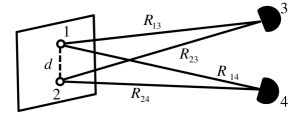
Figure 1: Two photons are emitted from two pinholes 1 and 2 separated by a distance $d$. Two detectors 3 and 4 are positioned in the far-field of the photons. There are two possible interfering processes by which the photons can reach the detectors. The interference between these paths leads to generation of entanglement.

Two point-like detectors 3 and 4 are positioned in the far-field of the pinholes. The photons reach the detectors after a time $r/c$, where their joint state (polarization) is measured. We are only interested in the events in which both detectors register a photon. For this geometry, the state of the photons at the detectors is pure and is given by

$$|\chi\rangle =\frac{1}{\sqrt{N}}\{\frac{e^{ik(R_{13}+R_{24})}}{R_{13}R_{24}}(a|H\rangle+b|V\rangle)\otimes(c|H\rangle+d|V\rangle)$$ (1)

$$+\frac{e^{ik(R_{23}+R_{14})}}{R_{23}R_{14}}(c|H\rangle+d|V\rangle)\otimes(a|H\rangle+b|V\rangle)\}$$

where $k=\omega/c$ is the wavenumber of the photons, $R_{ij}$ is the distance between source $i$ and detector $j$ and $N$ is the normalization constant. There are two interfering processes in which both detectors could register a single count: photon 1 landing on detector 3 and photon 2 on detector 4; photon 1 arriving at detector 4 and photon 2 at detector 3. The two terms in the sum may be interpreted as the two possible paths taken by the photons. In the far field of the sources where $R_{13}R_{24}\simeq R_{23}R_{14}$, the state vector simplifies to

$$|\chi\rangle = \frac{1}{\sqrt{N}}\{e^{-i\varphi}(a|H\rangle+b|V\rangle)\otimes(c|H\rangle+d|V\rangle)+$$ (2)

$$e^{i\varphi}(c|H\rangle+d|V\rangle)\otimes(a|H\rangle+b|V\rangle)\}$$

where $\varphi=\frac{k}{2}(R_{14}+R_{23}-R_{13}-R_{24})$ and we have assumed that the radial terms in the denominator of Eq. (1) are all of the same order in the far field and can be absorbed in the normalization $N$. The entanglement of this state can be quantified by concurrence Wootters (1998) and is given by

$$C=\frac{|(ad-cb)^{2}|}{2\cos^{2}{\varphi}(|ac|^{2}+|bd|^{2})+(|ad|^{2}+|cb|^{2}+2|abcd|\cos{\varphi})}.$$ (3)

As an example, if the photons begin in the state $|HV\rangle$, i.e. $a=d=1$ and $b=c=0$, one finds that the state at the detectors is $\frac{1}{\sqrt{2}}(|HV\rangle+|VH\rangle)$ and has entanglement of unity.

This apparently counterintuitive result occurs because both photons are radiated into a large solid angle: whether a photon landing on a detector originated at 1 or 2 is therefore unknown prior to measuring its polarization. We then post-select only those events in which both detectors register a count, projecting the detected state into a maximally entangled state.

II.2 General Case

The above analysis can be generalized for an initial state of the form $\alpha|HH\rangle+\beta|HV\rangle+\gamma|VH\rangle+\delta|VV\rangle$, i.e. an arbitrary pure state of the two incident photons, straightforwardly. The concurrence is now found to be

$$C=\frac{|\beta^{2}+\gamma^{2}+2\beta\gamma\cos{2\varphi}-4\alpha\delta\cos^{2}{\varphi}|}{1+\cos{(2\varphi)}(1-|\beta|^{2}-|\gamma|^{2}+2Re[\beta\gamma^{*}])}$$ (4)

As a first example, the entanglement of the initial state $\frac{1}{\sqrt{2}}(|HV\rangle+|VH\rangle)$ is invariant under propagation and the concurrence remains constant unity. The state $\frac{1}{\sqrt{2}}(|HV\rangle+i|VH\rangle)$, however, generates a state with concurrence of $|\cos{2\varphi}|$. Figure 2 shows a plot of concurrence versus the phase $\varphi$ for the initial states $|HV\rangle$ and $\frac{1}{\sqrt{2}}(|HV\rangle+i|VH\rangle)$. The entanglement of the initial state $\frac{1}{\sqrt{2}}(|HV\rangle+i|VH\rangle)$ is destroyed and revived as the path difference between the two possible paths for the photons to reach the detectors, is varied.

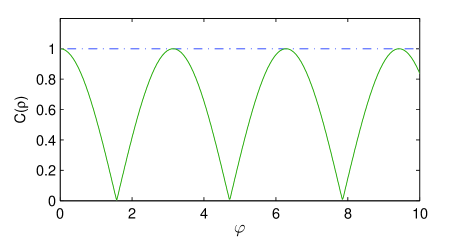
Figure 2: Far field entanglement versus the phase $\varphi$, for the initial states $\frac{1}{\sqrt{2}}(|HV\rangle+i|VH\rangle)$ (solid green line) and $|HV\rangle$(dashed blue line). Concurrence of the state generated from the initial state $\frac{1}{\sqrt{2}}(|HV\rangle+i|VH\rangle)$ takes the simple form $C(\rho)=|\cos(2\varphi)|$ in the far field.(Color online)

II.3 Beam-Splitter Analogy

Our scheme is reminiscent of standard entanglement generation schemes in linear optics where two photons are incident on a beam-splitter and the events in which the photons are separated into two different ports are post-selected (Fig. 3).

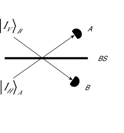
Figure 3: The state emerging from the beam-splitter is entangled provided that the photons are separated into two ports A and B.

We use the notation $|n_{i},m_{j}\rangle_{AB}\equiv|n_{i}\rangle_{A}|m_{j}\rangle_{B}$ to represent a two-photon state in which $n$($m$) $i$-polarized ($j$-polarized) photons are in the spatial mode $A$($B$), and each of the subscripts $i$ and $j$ can take two possible values: $H$ or $V$. For the incident state $|1_{H},1_{V}\rangle_{AB}$ the state emerging from the beam-splitter takes the form  Ou and Mandel (1988)

$$|\psi\rangle = \frac{1}{\sqrt{2}}\left(|1_{H},0\rangle_{AB}+i|0,1_{H}\rangle_{AB}\right)\otimes$$ (5)

$$\frac{1}{\sqrt{2}}\left(-i|1_{V},0\rangle_{AB}+|0,1_{V}\rangle_{AB}\right)$$

which is a product state and therefore not entangled. However, if we select the events in which two photons separate into the two output ports A and B, the resultant state is the maximally entangled state $\frac{1}{\sqrt{2}}\left(|1_{H},1_{V}\rangle_{AB}+|1_{V},1_{H}\rangle_{AB}\right)$. Similarly, free space propagation acts like a beam-splitter, combining the state of the two photons. The lack of the Hong-Ou-Mandel effect  Ou and Mandel (1988) in free space propagation, however, means that there is a subtle difference between the two schemes. To see this, consider a general state of the form $\alpha|1_{H},1_{H}\rangle_{AB}+\beta|1_{H},1_{V}\rangle_{AB}+\gamma|1_{V},1_{H}\rangle_{AB}+\delta|1_{V},1_{V}\rangle_{AB}$ incident on a beam- splitter. Post-selecting the events at which each detectors registers a count, we find the detected state to be $\frac{1}{\sqrt{2}}\left(|1_{H},1_{V}\rangle_{AB}+|1_{V},1_{H}\rangle_{AB}\right)$, provided that at least one of the amplitudes $\beta$ or $\gamma$ is non-zero. If both $\beta$ and $\gamma$ are zero, photon bunching prevents the photons from arriving at different ports. This is in sharp contrast to the case considered in the previous section where the entanglement of the detected state has a strong dependency on the amplitudes of the initial state.

Similar post-selective schemes have been utilized in linear optics quantum computing Knill et al. (2001); Kok et al. (2007); Adami and Cerf (1999) to generate entangled photons and perform logical operations or to induce effective non-linearities Lapaire et al. (2003). Since all such schemes rely on beam-splitters to erase the which-path information, their scalability is severely limited by interferometric stability; it would, therefore, be desirable to create multi-photon entangled states by simpler arrangements that do not rely on beam-splitters and/or Hong-Ou-Mandel effect.

III Two photon case: Emission by two atoms

Having established the role of interference between paths in entanglement creation/destruction, let us now consider a concrete example where the photons originate from spontaneous emission of two atoms. Apart from a means of implementing the scheme experimentally, this calculation places the heuristic argument presented above on firmer ground, and allows us to compute the entanglement at the intermediate points from the near-field to the far-field of the source. For a system consisting of two three-level atoms, interacting with a quantized field, the Hamiltonian in the rotating wave approximation is given by M:L

$$\hat{H}= \hbar\sum_{\mathbb{k},\lambda}{\omega}_{k}{\hat{a}_{\mathbb{k}\lambda}}^{\dagger}{\hat{a}_{\mathbb{k}\lambda}}+\hbar{\omega}_{0}\sum_{i}^{N}\sum_{\lambda}^{2}{\hat{s}_{\lambda i}}^{\dagger}{\hat{s}}_{\lambda i}+$$ (6)

$$\hbar\sum_{\mathbb{k},i,\lambda}g_{i,\mathbb{k},\lambda}\hat{a}_{\mathbb{k}\lambda}{{\hat{s}}_{\lambda i}}^{\dagger}+c.c.$$

where $\sum_{i}$ indicates summation over the atoms, $\sum_{\mathbb{k}}$ is the vector sum over the spatial field modes, $\sum_{\lambda}$ is the summation over the two orthogonal polarizations, $\hat{s}_{\lambda i}$ (${\hat{s}_{\lambda i}}^{\dagger}$) is the atomic lowering (raising) operator acting on the $i^{th}$ atom and corresponding to a transition with a $\lambda$ polarized photon, ${\hat{a}_{\mathbb{k}\lambda}}$ (${\hat{a}^{\dagger}_{\mathbb{k}\lambda}}$) is the field annihilation (creation) operator and $g_{i,\mathbb{k},\lambda}$ is the coupling constant. The two excited states are assumed to be degenerate with ${\omega}_{0}$ the atomic transition frequency. We choose to work in a basis where the atomic operators correspond to linearly polarized photons. Solving the Heisenberg equation of motion, $i\hbar\dot{\hat{s}}_{\lambda i}(t)=[\hat{s}_{\lambda i}(t),\hat{H}]$, we arrive at the following differential equation for the slowly varying amplitude ${\hat{A}}_{\alpha i}={\hat{s}}_{\alpha i}e^{i\omega_{0}t}$,

$$\frac{\partial{\hat{A}}_{\alpha i}}{\partial t}=i\frac{\gamma}{2}\sum_{j}M_{ij}{\hat{A}}_{\alpha j}(t)$$ (7)

where the matrix $M_{ij}$ describes the interaction between two atoms separated by $d$,

$$M_{ij}=\left\{\begin{array}[]{lr}0&i=j.\\ \frac{c}{d\omega_{0}}e^{i\omega_{0}d/c}&i\neq j\end{array}\right.$$ (8)

The solution to the differential equation is given by

$${\hat{s}}_{\alpha i}(t)=e^{-i\omega_{0}t}\sum_{p,n}{\zeta_{i}}^{(p)}{\zeta_{n}}^{(p)}e^{i\gamma\alpha_{p}t/2}e^{-\gamma(1+\beta_{p})t/2}{\hat{s}}_{\alpha i}(0)$$ (9)

where ${\zeta_{n}}^{(p)}$ is the $n^{th}$ eigenvector of the interaction matrix $M$, with eigenvalue $\alpha_{p}+i\beta_{p}$. In physical terms $\alpha_{p}$ and $\beta_{p}$ are the frequency shift and the decay shift due to super-radiant effects which are small if the atoms are more than one wavelength of radiation apart Dicke (1954) and may also be neglected. As a consequence of the orthogonality of the eigenvectors M:n , the Heisenberg equation for the atomic operators is reduced to ${\hat{s}}_{\alpha i}(t)={\hat{s}}_{\alpha i}(0)e^{-i{\omega}_{0}t}e^{-\gamma t/2}$ for $\alpha=1$ or $2$, which is equivalent to the solution of a classical oscillating dipole. The electric field at detector $j$ in the semi-classical approximation is given by the formula Lehmberg (1970)

$$\mathbb{\hat{E}_{j}}^{(+)}(r\mathbb{n_{j}},t)=\frac{p{{\omega}_{0}}^{2}}{4\pi{\epsilon}_{0}c^{2}}\sum^{2}_{l=1}\Bigg{(}\frac{\mathbb{n_{j}}\times[\mathbb{n_{j}}\times{\mathbb{\hat{s}}}_{l}(t^{{}^{\prime}}_{lj})]}{R_{lj}}$$

$$+~{}3(\mathbb{n_{j}}[\mathbb{n.\hat{s}}_{l}(t^{{}^{\prime}}_{lj})-\mathbb{\hat{s}}_{l}(t^{{}^{\prime}}_{lj})])\left(\frac{1}{{R_{lj}}^{3}}-\frac{ik}{{R_{lj}}^{2}}\right)\Bigg{)}$$ (10)

where $j=\{3,4\}$, $R_{lj}$ is the distance between atom $l$ and detector $j$, ${t^{{}^{\prime}}_{lj}}$ is the retarded time, $t^{{}^{\prime}}_{lj}=t-R_{lj}/c$, $\mathbb{\hat{s}_{l}}=(\hat{s}_{1l},\hat{s}_{2l},0)$, $p$ is the amplitude of the dipole moment of the atom and $\mathbb{n_{j}}$ is the unit vector in the direction of the observer. We have chosen the coordinates such that $\hat{s}_{1l}$($\hat{s}_{2l}$) is the component of the dipole moment operator along the x-axis (y-axis) (Fig. 4). We use $|x\rangle$, $|y\rangle$ and $|g\rangle$ to denote the eigenstates of the atomic operators, we can therefore write $\hat{s}_{11}\hat{s}_{12}|xx\rangle=|gg\rangle$, $\hat{s}_{21}\hat{s}_{12}|yx\rangle=|gg\rangle$ and so on. The radiated field may be simplified for an observer in the far-zone; however, since we are interested in computing the propagation of entanglement, all the terms in Eq. (10) will be kept. We compute the state vector of the post-selected two-photon state reaching the detectors for symmetric detection angles. The components of the electric field at detector $j$ decomposed along the azimuthal unit vectors $\mathbb{e_{\theta}}=(\cos{\phi}\cos{\theta},\sin{\phi}\cos{\theta},-\sin{\theta})$ and $\mathbb{e_{\phi}}=(-\sin{\phi},\cos{\phi},0)$ are given by

$$\hat{E}_{\phi j}^{(+)}(r\mathbb{n_{j}},t)=\frac{p{{\omega}_{0}}^{2}}{4\pi{\epsilon}_{0}c^{2}}\sum^{2}_{l=1}(\hat{s}_{yl}(t)\cos{\phi}-$$

$$\hat{s}_{xl}(t)\sin{\phi})\left(\frac{k^{2}}{R_{lj}}+\frac{1}{{R_{lj}}^{3}}-\frac{ik}{{R_{lj}}^{2}}\right)e^{ikR_{lj}}$$ (11)

$$\hat{E}_{\theta j}^{(+)}(r\mathbb{n_{j}},t)=\frac{p{{\omega}_{0}}^{2}}{4\pi{\epsilon}_{0}c^{2}}\sum^{2}_{l=1}(\hat{s}_{yl}(t)\cos{\theta}\sin{\phi}+$$

$$\hat{s}_{xl}(t)\cos{\phi}\cos{\theta})\left(\frac{k^{2}}{R_{lj}}+\frac{1}{{R_{lj}}^{3}}-\frac{ik}{{R_{lj}}^{2}}\right)e^{ikR_{lj}}$$ (12)

where $\hat{s}_{xl}\equiv\hat{s}_{1l}$ and $\hat{s}_{yl}\equiv\hat{s}_{2l}$ and the retarded dipole moment operator has been written as $\hat{s}(t-R_{lj}/c)=\hat{s}(t)e^{ikR_{lj}}$.

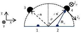
Figure 4: Two single photon sources $1$ and $2$ and two detectors $3$ and $4$ are positioned in the xz-plane as shown. The detectors are positioned symmetrically about the z-axis. The photon polarization is measured along the unit vectors $\hat{e}_{\theta}$ and $\hat{e}_{\phi}$.

We can simplify the calculations by remembering that all detected two-photon states are pure. A general (unnormalized) state reaching the detector is therefore of the form $|\chi\rangle=C_{\theta\phi}|HV\rangle+C_{\phi\theta}|VH\rangle+C_{\theta\theta}|HH\rangle+C_{\phi\phi}|VV\rangle$ where $|H\rangle$ and $|V\rangle$ represent the two linear polarizations in the detector basis, along the unit vectors $\mathbb{e}_{\theta}$ and $\mathbb{e}_{\phi}$ respectively. From the theory of photo-detection Glauber (1963) we know that $|C_{\theta\phi}|^{2}=\langle\psi|\hat{E}^{(-)}_{\theta 3}(r\mathbb{n_{3}})\hat{E}^{(-)}_{\phi 4}(r\mathbb{n_{4}})\hat{E}^{(+)}_{\theta 4}(r\mathbb{n_{4}})\hat{E}^{(+)}_{\phi 3}(r\mathbb{n_{3}})|\psi\rangle$ where $|\psi\rangle$ is the initial state of the atoms and, since $t=r/c$, we have omitted the time dependency of the fields. The amplitudes of the detected state are therefore given by

$$C_{\eta\kappa}=\langle gg|\hat{E}^{(+)}_{\eta 3}(r\mathbb{n_{3}})\hat{E}^{(+)}_{\kappa 4}(r\mathbb{n_{4}})|\psi\rangle$$ (13)

where $\eta$ and $\kappa$ can be $\theta$ or $\phi$ and $|gg\rangle$ is the ground state of the atoms.

As an example for the initial atomic states $|\psi_{1}\rangle=|xy\rangle$, $|\psi_{2}\rangle=\frac{1}{\sqrt{2}}(|xy\rangle+|yx\rangle)$ and $|\psi_{3}\rangle=\frac{1}{\sqrt{2}}(|xy\rangle+i|yx\rangle)$, where $|x\rangle$ and $|y\rangle$ represent the state of an atom in terms of the direction of its dipole moment, the detected two-photon states are respectively given by

$$|\chi_{1}\rangle=\frac{1}{\sqrt{2}}(|HV\rangle+e^{-2ikd\sin\theta}|VH\rangle)$$

$$|\chi_{2}\rangle=\frac{1}{\sqrt{2}}(|HV\rangle-|VH\rangle)$$

$$|\chi_{3}\rangle=-\frac{1}{2}\left(1+ie^{-2ikd\sin\theta}\right)|HV\rangle+\frac{1}{2}\left(i+e^{-2ikd\sin\theta}\right)|VH\rangle.$$

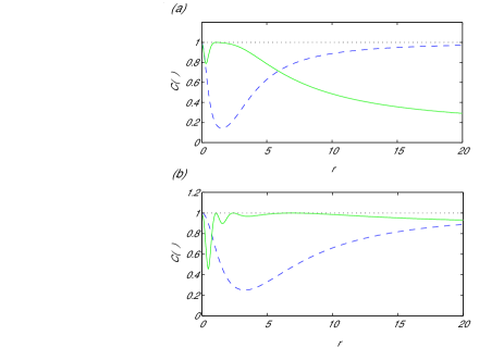
Figure 5: Concurrence versus the detector position r, in units of $\lambda/2\pi$ for $\theta=45^{\circ}$. The initial atomic states are $|xy\rangle$(dashed blue line) and $\frac{1}{\sqrt{2}}(|xy\rangle+i|yx\rangle)$(solid green line). a) $kd=3.45$ (far-field minimum) and b) $kd=7$ (far-field maximum).(Color online)

$|\chi_{1}\rangle$ and $|\chi_{2}\rangle$ have a concurrence of unity and $|\chi_{3}\rangle$ has concurrence of $|\cos{(2\varphi)}|$, in agreement with the heuristic treatment of the previous section. In fact, if the initial state of the atoms is an arbitrary state of the form $\alpha|xx\rangle+\beta|xy\rangle+\gamma|yx\rangle+\delta|yy\rangle$, one arrives at Eq. (4) for concurrence in the far-field.

We now compute the entanglement at all intermediate points as the detectors are moved from the near-field to the far-field. For a detection angle of $45^{\circ}$, the results are presented in Fig. (5). The behavior of the state $|xy\rangle$ is particularly intuitive to understand; at $r=0$ the detectors are at the origin and concurrence is unity due to complete mixing of photons. A “near-zone” minimum occurs at $r\sim\frac{d}{2}$ where a detector is positioned close to each atom and the probability of a photon captured by the farther detector is negligible. Concurrence then recovers its far-field value as the detectors are moved further apart. The state $|xy\rangle+i|yx\rangle$ also has unit concurrence at $r=0$, but no subsequent “near-zone” minimum. This is expected since the initial state was maximally entangled and the entanglement is directly transferred from the atoms to the photons if a detector is placed next to each atom. For $r<d/2$ a series of interference fringes occur as the detectors are moved apart. Concurrence recovers the far-zone value for $r>>d$.

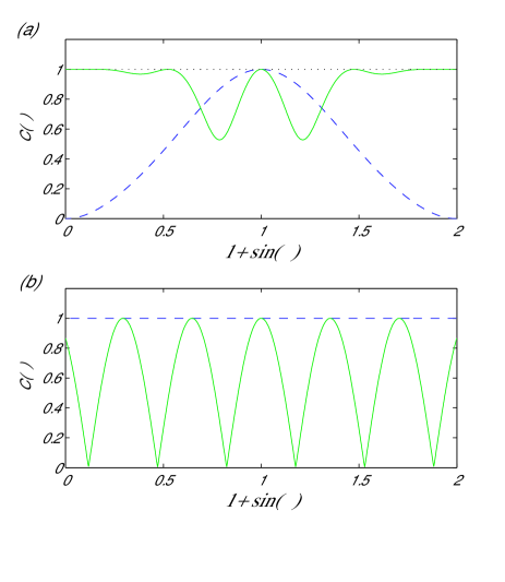
Figure 6: Concurrence for symmetric detector positions for the initial atomic states $|xy\rangle$(dashed blue line) and $\frac{1}{\sqrt{2}}(|xy\rangle+i|yx\rangle)$(solid green line). Both detectors make an angle $\theta$ with the z-axis, where $-\pi/2\leq\theta\leq\pi/2$. a) Concurrence in the near field for $kd=4.45$ and $r=2$. b) Concurrence in the far field for $kd=4.45$ and $r=1000$.(Color online)

Finally to see the spacial variation of entanglement, we move the detectors in the xz-plane, keeping them symmetric at all times, and plot the variation of concurrence as a function of the detection angle $\theta$ (Fig. 4). Figure 6a. shows the entanglement in the near-field. Figure 6b. is the corresponding plot in the far-field where we have chosen the atomic separation such that the state $\frac{1}{\sqrt{2}}(|xy\rangle+i|yx\rangle)$ would have maximum concurrence for a $\theta=45^{\circ}$ detection angle. The state $|xy\rangle$ generates maximally entangled photons for all symmetric detector orientations. Similar fringe patterns are observed at both extremes for the state $\frac{1}{\sqrt{2}}(|xy\rangle+i|xy\rangle)$, confirming the previous observations that altering the path difference between the photons can create maxima and minima of entanglement. Our results are consistent with the findings of Lim and Beige Lim and Beige (2005) who study the spacial variation of entanglement of formation for two dipole sources, but do not discuss the variation of entanglement at the intermediate points.

IV n-photon GHZ-states

IV.1 General Result

The above observations give rise to the question: can propagation and post-selection be used to create multi-photon entangled states? In this section, we first state a general symmetry property of any n-photon state that can be generated via propagation and post-selection in our chosen geometry. We then show how the initial conditions can be tailored to create n-photon GHZ states up to local unitaries. Finally we consider a three-photon GHZ state as a specific example.

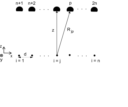
Figure 7: We consider an array of single photon emitters prepared in the state $|\psi\rangle=\sum_{i_{1}...i_{n}}D_{i_{1}...i_{n}}|i_{1}...i_{n}\rangle$. Polarization-resolving detectors are positioned in the far-field of the atoms with the same spacing as the atomic lattice.

We assume an arrangement consisting of a one-dimensional array of single photon emitters, separated by a distance $d$, with a single photon detector directly above each emitter a distance $z$ away (Fig. 7). We consider an initial state of the form $|\psi\rangle=\sum_{i_{1}...i_{n}}D_{i_{1}...i_{n}}|i_{1}...i_{n}\rangle$. After propagation and post-selection, this produces a final state of the form $|\chi\rangle=\sum_{i_{1}...i_{n}}C_{i_{1}...i_{n}}|i_{1}...i_{n}\rangle$ where, each of the subscripts can take two possible values, $H\equiv 0$ or $V\equiv 1$. We demonstrate that states with permutation symmetry can be generated from propagation of a suitable initial state, provided that the detectors are far enough from the source. Local unitaries may need to be applied on the photons before detection to create the desired entangled state. A state $|\chi\rangle=\sum_{i_{1}...i_{n}}C_{i_{1}...i_{n}}|i_{1}...i_{n}\rangle$ possess permutation symmetry if all amplitudes $C_{i_{1}...i_{n}}$ with different permutations of the subscripts are equal. The far-field condition is the key behind this result and assumes a first order approximation for the distance between each emitter and each detector; i.e. the phase difference between different paths is neglected. This demands $\frac{n^{2}d^{2}}{2z^{2}}\ll 1$ and becomes more difficult to satisfy for large $n$. The n-photon GHZ state $|GHZ\rangle_{n}=\frac{1}{\sqrt{2}}\left({|H\rangle}^{\otimes_{n}}-{|V\rangle}^{\otimes_{n}}\right)$, is an example of an state with the desired permutation symmetry; it can thus be created by simple spatial propagation, if the amplitudes of the initial state are chosen carefully. We demonstrate in Appendix A that propagation of the separable state

$$|\psi\rangle=\bigotimes_{l=1}^{n}\left(\sin\left(\frac{l\pi}{n}\right)|H\rangle+\cos\left(\frac{l\pi}{n}\right)|V\rangle\right)$$ (14)

generates the post-selected entangled state $|\chi\rangle$ up to global phases in the far-field such that

$$({\hat{{\mathcal{H}}}\hat{{\mathcal{S}}}^{\dagger})}^{{\otimes}^{n}}|\chi\rangle=\frac{1}{\sqrt{2}}\left({|H\rangle}^{\otimes_{n}}-{|V\rangle}^{\otimes_{n}}\right)$$ (15)

where $\hat{{\mathcal{H}}}$ is the Hadamard gate and $\hat{{\mathcal{S}}}$ is the phase gate such that $\hat{{\mathcal{S}}}|H\rangle=|H\rangle$, $\hat{{\mathcal{S}}}|V\rangle=i|V\rangle$, $\hat{{\mathcal{H}}}|H\rangle=\frac{1}{\sqrt{2}}(|H\rangle+|V\rangle)$ and $\hat{{\mathcal{H}}}|V\rangle=\frac{1}{\sqrt{2}}(|H\rangle-|V\rangle)$. Eq. (14) corresponds to an initial state of the atoms such that the polarization for the n-th emitted photon simply forms an angle of $\frac{180^{\circ}}{n}$ with the horizontal.

Assuming emission into a $4\pi$ solid angle and a total detection solid angle of $\Omega$, the probability of an $n$ photon coincidence is $P_{n}=n!\eta^{n}$ for $\eta=\eta_{q}\eta_{\Omega}$, where $\eta_{q}$ is the quantum efficiency of each detector and $\eta_{\Omega}=\Omega/(4\pi n)$ (assuming that the area of each detector scales as $\frac{1}{n}$). For large $n$, using Sterling’s formula for large factorials, one can show that the n-photon coincidence scales as $P_{n}\sim\sqrt{2\pi n}\left(\eta_{q}\Omega/(4\pi e)\right)^{n}$; in other words, it scales exponentially with the size of the array. The main drawback of the scheme, is therefore, the low probability of registering an n-photon coincidence. One possibility of overcoming this obstacle is to use classical interference to maximize the probability of detection at the desired detector locations and will be investigated in a subsequent publication.

IV.2 Three Photon GHZ state

As a concrete example and to elucidate Eq. (14) and Eq. (15), consider a general three-photon state of the form $|\psi\rangle=\sum_{\eta\kappa\epsilon}D_{\eta\kappa\epsilon}|\eta\kappa\epsilon\rangle$ which generates the state $|\chi\rangle=\sum_{\eta\kappa\epsilon}C_{\eta\kappa\epsilon}|\eta\kappa\epsilon\rangle$ in the far-field. By generalizing Eq. (13) the amplitudes of the detected state can be expressed as

$$C_{\eta\kappa\epsilon}=\langle ggg|\hat{E}^{(+)}_{\eta 4}(r\mathbb{n_{4}})\hat{E}^{(+)}_{\kappa 5}(r\mathbb{n_{5}})\hat{E}^{(+)}_{\eta 6}(r\mathbb{n_{6}})|\psi\rangle.$$ (16)

This equation can be simplified for an observer in the far-field. Inserting Eq. (III) and Eq. (III) into Eq. (16) for $\phi=0$, we arrive at the far-limit of Eq. (16)

$$C_{\eta\kappa\xi}=\langle ggg|\sum_{lmn}\sum_{\alpha\beta\gamma}D_{\alpha\beta\gamma}\hat{s}_{\eta l}\hat{s}_{\kappa m}\hat{s}_{\xi n}|\alpha\beta\gamma\rangle.$$ (17)

For the arrangement considered $R_{ji}\cong z$ for all $i$ and $j$ in the far-field and therefore all radial terms have dropped out. The amplitude $C_{\eta\kappa\xi}$ is therefore the sum of six terms: all cyclic and anti-cylic permutations of $\eta$, $\kappa$ and $\xi$:

$$C_{\eta\kappa\xi}=D_{\eta\kappa\xi}+D_{\kappa\xi\eta}+D_{\xi\eta\kappa}+D_{\eta\xi\kappa}+D_{\kappa\eta\xi}+D_{\xi\kappa\eta}$$ (18)

This immediately proves, for example, that the state $|HHV\rangle$ generates a $W$ state in the far-field. To see how GHZ states are created, one must demonstrate that propagation of the initial state $|\psi\rangle=\bigotimes_{l=1}^{3}(\sin(\frac{l\pi}{3})|H\rangle+\cos(\frac{l\pi}{3})|V\rangle)$ generates the state $|\chi\rangle=\sum_{\eta\kappa\epsilon}C_{\eta\kappa\epsilon}|\eta\kappa\epsilon\rangle=\frac{1}{2}(|HHV\rangle+|HVH\rangle+|VHH\rangle-|VVV\rangle)$ in the far-field. To prove this it is sufficient to show that a) $C_{001}=C_{010}=C_{100}=-C_{111}$, b) $C_{110}=C_{101}=C_{011}=0$ . Both these criteria can readily be verified from Eq. (18).

Three qubit GHZ states have genuine tri-partite entanglement Coffman et al. (2000) and show maximum violation of three-qubit Bell inequality Gho . Three-tangle is a measure of genuine tri-partite entanglement and is defined to be Coffman et al. (2000)

$$\tau={\cal{C}}_{1(23)}^{2}-{\cal{C}}_{12}^{2}-{\cal{C}}_{13}^{2}$$ (19)

where ${\cal{C}}_{ij}$ is the concurrence between qubits $i$ and $j$ and ${\cal{C}}_{1(23)}$ measures the entanglement between qubit 1 and the joint state of qubits 2 and 3. Three-tangle is bounded between 0 and 1 and states equivalent to GHZ states up to local unitaries are characterized by a three-tangle of unity. Figure 8 is a plot of three-tangle versus distance for the initial state $|\psi\rangle=\bigotimes_{l=1}^{n}(\sin(\frac{l\pi}{n})|H\rangle+\cos(\frac{l\pi}{n})|V\rangle)$ for two different initial atomic spacings. In the far-field all phase information is washed out and three-tangle approaches unity independent of the initial separation as expected.

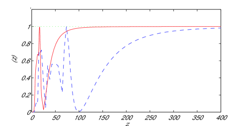
Figure 8: Three-tangle versus the perpendicular detector position $z$ in units of $\lambda/2\pi$ for the initial state described by Eq. (14) (n=3) for $d=\lambda$ (solid red line) and $d=2\lambda$ (dashed blue line).

V Conclusion

In conclusion, we have demonstrated that entanglement of photons emitted in a large solid angle can change on propagation. This arises because in the far-zone all information about the origin of the photons is lost and this leads to quantum mechanical interference between all possible paths to the detectors. We use concurrence and three-tangle as measures of two and three qubit entanglement and verify that both these quantities vary smoothly from near-field to far-field. We demonstrate that the propagation of the state $|\psi\rangle=\bigotimes_{l=1}^{n}(\sin(\frac{l\pi}{n})|H\rangle+\cos(\frac{l\pi}{n})|V\rangle)$ generates n-photon GHZ states post-selectively. Our results appear to suggest that the chosen geometry is suitable for generation of states with permutation symmetry; both n-photon W and GHZ states fall into this category.

The scheme may be realized experimentally using quantum dots or ions prepared in arbitrary initial states. The main drawback of the scheme is that the entangled photons are only accessible via post-selective or non-demolition measurements, which makes the scheme, in its current form, of limited use in practical generation of entanglement. However, generation of effective interactions between photons without the need for beam-splitters has obvious attractions in the design of linear optics quantum processors. One possibility of overcoming the post-selectivity criterion is using classical interference to maximize the probability of photon detection at the desired detector locations. This possibility is currently under investigation.

APPENDIX A: n-photon GHZ-states

Here we present the proof that for a particular choice of the initial state, the state reaching the detector is an n-photon GHZ state up to local unitary rotations. We adopt the binary notation to denote the polarization states,

$$|0\rangle\equiv|H\rangle$$ (20)

$$|1\rangle\equiv|V\rangle.$$ (21)

Theorem: For the specific geometry shown in Fig.7 propagation of the state

$$|\psi\rangle=\bigotimes_{l=1}^{n}\left(\sin\left(\frac{l\pi}{n}\right)|0\rangle+\cos\left(\frac{l\pi}{n}\right)|1\rangle\right)$$ (22)

post-selectively generates the state $|\chi\rangle$ up to global phases in the far-field such that

$$({\hat{{\mathcal{H}}}\hat{{\mathcal{S}}}^{\dagger})}^{{\otimes}^{n}}|\chi\rangle=\frac{1}{\sqrt{2}}\left({|0\rangle}^{\otimes_{n}}-{|1\rangle}^{\otimes_{n}}\right)$$ (23)

where the far-field is defined by the condition $\frac{n^{2}d^{2}}{2z^{2}}\ll 1$, $\hat{{\mathcal{H}}}$ is the Hadamard gate and $\hat{{\mathcal{S}}}$ is the phase gate such that $\hat{{\mathcal{S}}}|0\rangle=|0\rangle$ and $\hat{{\mathcal{S}}}|1\rangle=i|1\rangle$, $\hat{{\mathcal{H}}}|0\rangle=\frac{1}{\sqrt{2}}(|0\rangle+|1\rangle)$, $\hat{{\mathcal{H}}}|1\rangle=\frac{1}{\sqrt{2}}(|0\rangle-|1\rangle)$.

Proof: Let us assume initially that n is odd. The initial state $|\psi\rangle$ and the final state $|\chi\rangle$ can be rewritten as $|\psi\rangle=\sum_{i_{1}...i_{n}}D_{i_{1}...i_{n}}|i_{1}...i_{n}\rangle$ and $|\chi\rangle=\sum_{i_{1}...i_{n}}C_{i_{1}...i_{n}}|i_{1}...i_{n}\rangle$. By generalizing Eq. (18) we have

$$C_{i_{1}...i_{n}}=\sum_{n!~{}perm.}D_{i_{1}...i_{n}}$$ (24)

where the summation is carried out over all $n!$ possible permutations of the subscripts. The detected state possesses permutation symmetry; meaning that all amplitudes with different permutations of the same subscripts are equal. We use the notation ${\cal{C}}_{n,m}$ to denote the amplitude of an $n$-photon state in which $m$ are in the state 1. We must show that the detected state with no rotation is of the form

$$({\hat{{\mathcal{S}}}}{\hat{{\mathcal{H}}}})^{{\otimes}^{n}} \frac{1}{\sqrt{2}} \left(|00...0\rangle-|11...1\rangle\right)=$$ (25)

$$\frac{i}{\sqrt{N}}\sum_{i_{1}...i_{n}}B_{i_{1}...i_{n}}|i_{1}...i_{n}\rangle$$

where the amplitudes are symmetric with respect to permutations and can be expressed as

$${\cal{B}}_{n,m}=\left\{\begin{array}[]{lr}0&m~{}even\\ (-1)^{\frac{m-1}{2}}&m~{}odd.\end{array}\right.$$ (26)

The strategy is to prove that ${\cal{C}}_{n,m}\equiv{\cal{B}}_{n,m}$. In order to do so we must show that: a)${\cal{C}}_{n,m}=0$ for all even m, b) $\frac{{\cal{C}}_{n,m}}{{\cal{C}}_{n,1}}=(-1)^{\frac{m-1}{2}}$ for all odd $m$ with $n>m$.

Condition a. The amplitudes $D_{i_{1}...i_{n}}$ can be written as $D_{i_{1}...i_{n}}=\Pi_{j=1}^{j=n}f(\frac{j\pi}{n}.i_{j})$ where the function $f(x.i_{j})$ is defined to be

$$f(x.i_{j})=\left\{\begin{array}[]{lr}\sin(x)&\mbox{if}~{}~{}i_{j}=0\\ \cos(x)&\mbox{if}~{}~{}i_{j}=1\end{array}\right.$$ (27)

We therefore have $C_{i_{1}...i_{n}}=\sum_{n!~{}perm.}\prod_{j=1}^{j=n}f\left(\frac{j\pi}{n}.i_{j}\right)$. Since $i_{n}=1$ we can exclude the last photon and write

$$C_{i_{1}...i_{n}}=\sum_{(n-1)!~{}perm.}\prod_{j=1}^{n-1}f\left(\frac{j\pi}{n}.i_{j}\right)$$ (28)

which vanishes if the product contains an odd number of cosines, or an even number of 1s (including the $i_{n}$ photon). To see this consider the amplitude ${\cal{C}}_{n,2}$. Expanding Eq. (28) we arrive at

$${\cal{C}}_{n,2}=\Bigg{(}\sum_{i=1}^{\frac{n-1}{2}}\sin{(\frac{i\pi}{n})}\cos{(\frac{i\pi}{n})}\prod_{j=1,j\neq i}^{\frac{n-1}{2}}\sin^{2}(\frac{j\pi}{n})+$$

$$\sum_{i=\frac{n+1}{2}}^{n-1}\sin{(\frac{i\pi}{n})}\cos{(\frac{i\pi}{n})}\prod_{j=\frac{n+1}{2},j\neq i}^{n-1}\sin^{2}{(\frac{j\pi}{n})}\Bigg{)}(n-2)!2!$$

which vanishes since $\sin(\frac{i\pi}{n})=\sin(\frac{n-i}{n}\pi)$ and $\cos(\frac{i\pi}{n})=-\cos(\frac{n-i}{n}\pi)$. This proves condition a.

Condition b. We now write expressions for ${\cal{C}}_{n,1}$ and ${\cal{C}}_{n,m}$, excluding all vanishing terms in Eq. (28) we obtain

$${\cal{C}}_{n,1}=(n-1)!\prod_{i=1}^{\frac{n-1}{2}}\sin^{2}{\left(\frac{i\pi}{n}\right)}$$ (29)

and

$${\cal{C}}_{n,m}=(-1)^{m^{\prime}}(n-m)!m!\sum_{i_{1}>i_{2}>...i_{m^{\prime}}}^{\frac{n-1}{2}}\cos^{2}{\left(\frac{i_{1}\pi}{n}\right)}...$$

$$\cos^{2}{(\frac{i_{m^{\prime}}\pi}{n})}\prod_{k\neq i_{\alpha},\alpha=1,..m^{\prime}}^{\frac{n-1}{2}}\sin^{2}{\left(\frac{k\pi}{n}\right)}$$ (30)

where $m^{\prime}=\frac{m-1}{2}$. The ratio of ${\cal{C}}_{n,1}$ and ${\cal{C}}_{n,m}$ is therefore given by

$$\frac{{\cal{C}}_{n,m}}{{\cal{C}}_{n,1}}=(-1)^{\frac{m-1}{2}}\sum_{i_{1}>i_{2}...>i_{m^{\prime}}}^{\frac{n-1}{2}}\cot^{2}{\left(\frac{i_{1}\pi}{n}\right)}\cdots$$

$$\cot^{2}{\left(\frac{i_{m^{\prime}}\pi}{n}\right)}\frac{(n-m)!m!}{(n-1)!}.$$ (31)

Condition b therefore demands:

$$\sum_{i_{1}>i_{2}>...i_{m^{\prime}}}^{\frac{n-1}{2}}\cot^{2}{(\frac{i_{1}\pi}{n})}\cdots\cot^{2}{(\frac{i_{m^{\prime}}\pi}{n})}\equiv\frac{(n-1)!}{m!(n-m)!}$$ (32)

This equation can be proven by recalling that $t_{r}=\cot^{2}{(\frac{r\pi}{2p+1})}$ for $r=1,2,...p$ are the distinct roots of the $p$th degree polynomial Aigner and Ziegler (2003)

$$Q(t):=\sum_{k=0}^{p}{2p+1\choose 2k+1}(-1)^{k}t^{p-k}$$ (33)

where ${n\choose k}=\frac{n!}{k!(n-k)!}$ . By applying Viéte’s formula Vinberg (2003) to Eq. (33) and making the substitution $p=\frac{n-1}{2}$ and $m=\frac{m-1}{2}$ we arrive at Eq. (32). This proves condition b.

If $n$ were assumed to be even from the outset, the upper limit of the sum in Eq. (32) would have been $\frac{n}{2}-1$. The proof for even n would have then demanded the substitution $p=\frac{n}{2}-1$ in Eq. 33.

References

- Mandel and Wolf (1995) L. Mandel and E. Wolf, Optical Coherence and Quantum Optics (Cambridge University Press, p.180, 1995).
- van Cittert (1934) P. H. van Cittert, Physica 1, 201 (1934).
- Zernike (1938) F. Zernike, Physica 5, 785 (1938).
- Wolf (1987) E. Wolf, Nature (London) 326, 363 (1987).
- Wolf and James (1996) E. Wolf and D. F. V. James, Rep. Prog. Phys. 59, 771 (1996).
- James (1994) D. F. V. James, J. Opt. Soc. Am. A 11, 1641 (1994).
- Lim and Beige (2005) Y. L. Lim and A. Beige, J. Phys. A 38, L7 (2005).
- Eibl et al. (2003) M. Eibl, S. Gaertner, M. Bourennane, C. Kurtsiefer, M. Zukowski, and H. Weinfurter, Phys. Rev. Lett. 90, 200403 (2003).
- Fattal et al. (2004) D. Fattal, K. Inoue, J. Vuckovic, C. Santori, G. S. Solomon, and Y. Yamamoto, Phys. Rev. Lett. 92, 037903 (2004).
- Pan et al. (2001) J.-W. Pan, M. Daniell, S. Gasparoni, G. Weihs, and A. Zeilinger, Phys. Rev. Lett. 86, 4435 (2001).
- Cabrillo et al. (1999) C. Cabrillo, J. I. Cirac, P. García-Fernández, and P. Zoller, Phys. Rev. A 59, 1025 (1999).
- Matsukevich et al. (2008) D. N. Matsukevich, P. Maunz, D. L. Moehring, S. Olmschenk, and C. Monroe, Phys. Rev. Lett. 100, 150404 (2008).
- Coffman et al. (2000) V. Coffman, J. Kundu, and W. K. Wootters, Phys. Rev. A 61, 052306 (2000).
- Lu et al. (2007) C.-Y. Lu, X.-Q. Zhou, O. G hne, W.-B. Gao, J. Zhang, Z.-S. Yuan, A. Goebel, T. Yang, and J.-W. Pan, Nature Physics 3, 91 (2007).
- Knill et al. (2001) E. Knill, R. Laflamme, and G. J. Milburn, Nature (London) 409, 46 (2001).
- Kok et al. (2007) P. Kok, W. J. Munro, K. Nemoto, T. C. Ralph, J. P. Dowling, and G. J. Milburn, Rev. Mod. Phys. 79, 135 (2007).
- Raussendorf and Briegel (2001) R. Raussendorf and H. J. Briegel, Phys. Rev. Lett. 86, 5188 (2001).
- Briegel et al. (2009) H. J. Briegel, D. E. Browne, W. Duer, R. Raussendorf, and M. V. den Nest, Nature Physics 5, 19 (2009).
- Browne and Rudolph (2005) D. E. Browne and T. Rudolph, Phys. Rev. Lett. 95, 010501 (2005).
- Prevedel et al. (2007) R. Prevedel, M. S. Tame, A. Stefanov, M. Paternostro, M. S. Kim, and A. Zeilinger, Phys. Rev. Lett. 99, 250503 (2007).
- (21) S. J. Devitt, A. G. Fowler, A. M. Stephens, A. D. Greentree, L. C. L. Hollenberg, W. J. Munro, K. Nemoto, arxiv:0808.1782.
- Wootters (1998) W. K. Wootters, Phys. Rev. Lett. 80, 2245 (1998).
- Ou and Mandel (1988) Z. Y. Ou and L. Mandel, Phys. Rev. Lett. 61, 50 (1988).
- Adami and Cerf (1999) C. Adami and N. J. Cerf, Quantum Computing and Quantum Communications (Springer Berlin, 391-401, 1999).
- Lapaire et al. (2003) G. G. Lapaire, P. Kok, J. P. Dowling, and J. E. Sipe, Phys. Rev. A 68, 042314 (2003).
- (26) This is a three-level generalization of the two-level Hamiltonian in R. H. Lehmberg, Phys. Rev. A 2, 883 (1970).
- Dicke (1954) R. H. Dicke, Phys. Rev. 93, 99 (1954).
- (28) Matrix is non-hermetian symmetric, the left and the right eigenvectors are therefore equal and we have , .
- Lehmberg (1970) R. H. Lehmberg, Phys. Rev. A 2, 883 (1970).
- Glauber (1963) R. J. Glauber, Phys. Rev. 130, 2529 (1963).
- (31) S. Ghose, N. Sinclair, S. Debnath, P. Rungta, R. Stock, arXiv:quant-ph/0812.3695.
- Aigner and Ziegler (2003) M. Aigner and G. M. Ziegler, Proofs from THE BOOK (Berlin; New York: Springer, p.45, 2003).
- Vinberg (2003) E. B. Vinberg, A course in algebra (American Mathematical Society, 2003).