Optimising Boltzmann codes for the PLANCK era

Abstract

High precision measurements of the Cosmic Microwave Background (CMB) anisotropies, as can be expected from the planck satellite, will require high-accuracy theoretical predictions as well. One possible source of theoretical uncertainty is the numerical error in the output of the Boltzmann codes used to calculate angular power spectra. In this work, we carry out an extensive study of the numerical accuracy of the public Boltzmann code CAMB, and identify a set of parameters which determine the error of its output. We show that at the current default settings, the cosmological parameters extracted from data of future experiments like Planck can be biased by several tenths of a standard deviation for the six parameters of the standard $\Lambda$CDM model, and potentially more seriously for extended models. We perform an optimisation procedure that leads the code to achieve sufficient precision while at the same time keeping the computation time within reasonable limits. Our conclusion is that the contribution of numerical errors to the theoretical uncertainty of model predictions is well under control – the main challenges for more accurate calculations of CMB spectra will be of an astrophysical nature instead.

1 Introduction

Any meaningful quantitative analysis of experimental data is based on a comparison with the predictions of a theoretical model, and the analysis of Cosmic Microwave Background (CMB) anisotropies is no exception to this rule. The amount of information to be gained from observations is limited not only by experimental uncertainties (such as detector noise, foregrounds, etc.), but also by the ability to accurately predict observable quantities from a given theory. There are various sources of theoretical uncertainties. Some, such as cosmic variance, are endemic to the problem, and unavoidable. Others are based on insufficient theoretical understanding of the complex processes involved [1] (examples include the physics of recombination [2], reionisation [3], and contributions due to the Sunyaev-Zel’dovich effects). Additionally, the analysis may be compromised by inaccuracies in the numerical programmes used to calculate the anisotropy angular power spectra [4].

With increasingly sophisticated experiments, and the contribution from experimental errors becoming less and less important, the relative significance of theoretical errors increases. In fact, for the planck satellite [5], the signal uncertainty of the temperature anisotropies will be dominated by cosmic variance instead of noise over a wide range of scales up to multipoles of $\ell\simeq 2000$.

Ignoring any type of uncertainty can lead to biased estimates of parameter values, and, in the worst case, a wrong physical interpretation of the data. It is therefore imperative to either make sure that the errors are small enough to be negligible, or, if that should not be the case, to devise an appropriate strategy to deal with the problem.

In the present work, we shall consider the numerical accuracy of the Boltzmann codes employed to calculate the angular anisotropy spectra $\mathcal{C}_{\ell}$ for given input values of cosmological parameters. The first public Boltzmann code was released more than a decade ago [6], and to date, there are several other such programmes freely available for download [7, 8, 9]. The output of all these codes is necessarily inaccurate to some extent, due to the use of semi-analytical approximations as well as artifacts of the numerical implementation, such as finite integration steps or the need to interpolate. These effects can be parameterised by a set of accuracy parameters, whose settings determine the accuracy of the output, but also the computation time. Here, we will focus our analysis on the CAMB code by Lewis, Challinor and Lasenby [8] in order to avoid possible systematic effects caused by differences between codes – a comparison of different (more or less) independent Boltzmann codes was performed by Seljak et al. [4], who found an excellent qualitative agreement. We extend their line of reasoning and present a detailed analysis of the potential effects of numerical inaccuracies on parameter estimates from planck data. Additionally, we optimise the accuracy settings of CAMB to find an ideal balance between precision and execution time.

We proceed in Section 2 by defining an appropriate measure of accuracy, identifying the relevant parameters which affect the accuracy of the output spectra and constructing a set of CMB reference spectra. In Section 3, we will describe our optimisation procedure and present a recommended set of accuracy parameters for CAMB, followed by an analysis of the expected potential bias on the cosmological parameters of the vanilla model caused by numerical inaccuracies in Section 4. The impatient reader may prefer to skip directly to our conclusions in Section 5.

2 Reference spectra

2.1 The fiducial model

In principle, the impact of individual accuracy parameters and the number of relevant parameters will depend on the underlying cosmological model assumed, and on the values of the cosmological parameters. In this analysis, we will stick to the 6-parameter $\Lambda$CDM-“vanilla”-model and we limit ourselves to a point in the space of cosmological parameters that lies close to the best fit to the WMAP 5-year data [10], see Table 1. We neglect the effects of weak gravitational lensing on the CMB spectra [11] (which will of course have to be taken into account in an analysis of real planck data), and ignore signatures of non-minimal models, like massive neutrinos, tensor modes, spatial curvature, etc., and defer their treatment to future work.

Table 1: Free cosmological parameters of the model, fiducial values used to generate the mock data, and prior ranges adopted in the analysis of Section 4.

Parameter		Fiducial Value	Prior Range
Dark matter density	$\Omega_{\rm dm}h^{2}$	0.10976	$0.01\to 0.99$
Baryon density	$\Omega_{\rm b}h^{2}$	0.02303	$0.005\to 0.1$
Hubble parameter	$h$	0.7	$0.4\to 1$
Optical depth to reionisation	$\tau$	0.09	$0.01\to 0.5$
Scalar spectral index	$n_{\mathrm{S}}$	0.96	$0.5\to 1.5$
Amplitude of scalar spectrum @ $k=0.05$ Mpc-1	$\ln\left[10^{10}A_{\mathrm{S}}\right]$	3.135	$3\to 4$

2.2 Measuring accuracy

In order to quantify the accuracy of the Boltzmann code output $\mathcal{C}_{\ell}^{\rm out}$, we require two things: a reference point $\mathcal{C}_{\ell}^{\rm ref}$ to compare with, and a measure of accuracy.

The reference spectra $\mathcal{C}_{\ell}^{\rm ref}$ would ideally be the exact prediction of the theory. In practice however, we have to make do with getting close enough to these ideal spectra. We will return to this issue and describe the construction of $\mathcal{C}_{\ell}^{\rm ref}$ in 2.4.

To measure accuracy, one might be tempted at first glance to look at the relative difference of the spectra $(\mathcal{C}_{\ell}^{\rm out}-\mathcal{C}_{\ell}^{\rm ref})/\mathcal{C}_{\ell}^{\rm ref}$ for each $\ell$. However, this approach does not properly take into account the fact that the accuracy requirements are dependent on $\ell$ (due to cosmic variance and experimental errors). Additionally, the spectra are merely an intermediate step in the inference process. In the end, we are interested in possible biases on cosmological parameters, not the accuracy of the spectra. A more meaningful measure of deviation from the reference spectra is the effective $\chi^{2}$, which can be obtained by using the reference spectra to generate a fiducial data set, taking into account the experimental errors of an experiment (or the projected errors in case of future experiments), and “fitting” $\mathcal{C}_{\ell}^{\rm out}$ to these data.

More formally, the effective $\chi^{2}$ is related to the likelihood $\mathcal{L}$ and defined by

$$\chi^{2}=-2\ln\mathcal{L}=\sum_{\ell}(2\ell+1)\left[\Tr\left(\mathbf{\tilde{C}_{\ell}}^{-1}\mathbf{\hat{C}_{\ell}}\right)+\ln\frac{\left|\mathbf{\tilde{C}_{\ell}}\right|}{\left|\mathbf{\hat{C}_{\ell}}\right|}-2\right].$$ (2.1)

Here, $\mathbf{\tilde{C}_{\ell}}$ is the theoretical covariance matrix, and its entries are taken to be the sum of the signal and noise power spectra:

$$\mathbf{\tilde{C}}_{\ell}=\left\{\mathcal{C}_{\ell}^{XX^{\prime}}+\mathcal{N}_{\ell}^{XX^{\prime}}\right\},$$ (2.2)

where the index $X$ runs over temperature ($T$) and polarisation ($E$), and for a fiducial data set, we can take the data covariance matrix $\mathbf{\hat{C}_{\ell}}$ to be equal to $\left.\mathbf{\tilde{C}_{\ell}}\right|_{\theta_{0}}$, i.e., the theoretical covariance matrix evaluated for the fiducial values of the cosmological parameters.

We take the noise to be isotropic and Gaussian; the noise power spectrum is related to the experimental parameters of Table 2 through

$$\mathcal{N}_{\ell}^{XX^{\prime}}=\delta_{XX^{\prime}}\;\theta_{\rm beam}^{2}\,\Delta_{X}^{2}\,\exp\left[\ell\left(\ell+1\right)\frac{\theta_{\rm beam}^{2}}{8\ln 2}\right].$$ (2.3)

For more details see Refs. [12, 13]. It should be noted that the normalisation of Eq. (2.1) is chosen such that the total $\chi^{2}$ is zero when the output spectra exactly match the reference spectra used to construct the fiducial data.

We generate the fiducial data set of $TT$-, $EE$-, and $TE$-spectra up to $\ell=3000$ using the code of Perotto et al. [12]. For simplicity we ignore the effects of incomplete sky coverage due to masking the galaxy and point sources, as well as anisotropic noise [14]. To evaluate the accuracy of CAMB in view of the expected data from planck, we assume 14 months of integrated observations in the 70 GHz channel of LFI and the 100 and 143 GHz channels of the HFI instrument; their specifications are taken from the planck blue book [5] and listed in Table 2.

2.2.1 Interpretation of the $\chi^{2}$ measure

As can be seen in Eq. 2.1, $\chi^{2}$ is directly related to the likelihood, which, along with a choice of prior probability densities on all cosmological parameters, leads to the posterior probability density, from which constraints on parameters are eventually derived. Assuming flat priors on the parameters and a multivariate Gaussian likelihood function, for a given numerical error $\chi^{2}$, the bias on any cosmological parameter cannot exceed $\sqrt{\chi^{2}}$ standard deviations in the worst case (i.e., when the error in the angular power spectra can be exactly offset by changing one of the cosmological parameters). On the other hand, if the error had no degeneracy with any cosmological parameter, the effect of a non-zero $\chi^{2}$ would be just a constant offset to the likelihood function, which would not have any effect on parameter inference. In realistic cases, the expected bias would lie somewhere in between. For the parameters of the vanilla model, we will provide an estimate of the bias in Section 4.

Table 2: List of technical specifications for the 70 GHz channel of the LFI and the 100 and 143 GHz channels of the HFI instrument: $\theta_{\rm beam}$ denotes the beam width, $\Delta_{T,P}$ are the sensitivities per pixel and $\nu$ is the centre frequency of the channels.

$\nu$/GHz	$\theta_{\rm beam}$	$\Delta_{T}$/$\mu$K	$\Delta_{P}$/$\mu$K
70	14.0’	12.8	18.3
100	9.5’	6.8	10.9
143	7.1’	6.0	11.4

2.3 The accuracy parameters

The numerical accuracy of a Boltzmann code’s output depends on many factors, ranging from the use of analytical approximations to the sampling various intermediate quantities in the calculation. These sources of numerical error can be quantified in terms of accuracy parameters, e.g., the number of samples used for interpolating a particular quantity. An increase in accuracy will generally be accompanied by a longer computation time and possibly higher requirements on the available computer memory.

We use the June 2008 version of CAMB as a starting point of our analysis. The unmodified version of CAMB comes with a set of three continuously adjustable accuracy parameters:

• l_sample_boost: determines for which values of $\ell$ the $\mathcal{C}_{\ell}$ are actually calculated (the rest are interpolated).

• l_accuracy_boost: determines the multipole at which the Boltzmann hierarchy for photons, neutrinos, etc., is cut off.

• accuracy_boost: affects the setting of various time steps, samplings, etc.

The latter two parameters affect several settings at once, so in the interest of optimising the performance of CAMB, we split them up into their constituents and treat them separately. Apart from the settings governed by these three parameters, we identified a few other quantities which can affect the accuracy of the results, and should be taken into account when optimising the code. Altogether, we consider a set of 19 accuracy parameters in our analysis, listed in Table 3.

All parameters are defined in such a way that setting them a value of 1 reproduces the results of the unmodified version of CAMB, and larger values correspond to better accuracy. The constituents of the old l_accuracy_boost and accuracy_boost parameters are taken to multiply the old l_accuracy_boost and accuracy_boost parameters (e.g., setting $\texttt{lmaxg}=\texttt{lmaxnr}=2$ produces the same effect as setting $\texttt{l\_accuracy\_boost}=2$). We modified the routine that determines for which values of $\ell$ the $\mathcal{C}_{\ell}$ are calculated: our parameter new_l_sample_boost is defined to be the square root of the old l_sample_boost; for $\texttt{new\_l\_sample\_boost}>5$, all $\mathcal{C}_{\ell}$ are calculated and there will be no interpolation of the final spectrum.

Table 3: Individual accuracy parameters for CAMB-CAMB comparison.

Parameter	Corresponding old accuracy parameter	Description and comments
new_l_sample_boost	l_sample_boost	$\ell$-sampling of $\mathcal{C}_{\ell}$s
lmaxg	l_accuracy_boost	Boltzmann hierarchy cutoff for photons
lmaxnr		Boltzmann hierarchy cutoff for massless neutrinos
int_tol		tolerance parameter for integration routines
ri_timestep		time step during reionisation
rec_timestep		time step during recombination
rec_timestep2		time step between recombination and reionisation
rad_trunc		truncation of photon hierarchy during matter domination
dec_start	accuracy_boost	starting time of decoupling
int_sample		samples for integration over source function
source_dk		$k$-sampling of source function
source_kmin		minimum value of $k$ to calculate source function for
int_xlmax1		starting time for source function integration
tc_largek		switch off tight coupling later for large $k$
tc_ep0	–	tight coupling switch
bess_sampling	–	$x$-sampling of spherical Bessel functions $j_{\ell}(x)$
bess_xlimmin	–	approximate $j_{\ell}(x)\simeq 0$ for small $x$, if $\ell\geq\texttt{xlimmin}$
bess_xlimfrac	–	approximate $j_{\ell}(x)\simeq 0$ for large $\ell$, if $x\leq(1-\texttt{xlimfrac})\cdot\ell$
ketamax	–	maximum value of $k\eta$

2.4 Constructing a reference data set

To quantify absolute accuracy we require a reference data set, as discussed above. Its construction is naturally tied to choosing the accuracy parameters in such a way that increasing them further would not have any appreciable effect. However, by arbitrarily increasing all parameters to “large” values at the same time, one would run into the limits of the hardware, particularly the available memory. For the purpose of finding suitable values for generating the reference spectra, we therefore analyse the parameters one by one, keeping all other parameters fixed. For each parameter, we generate a fiducial reference data set with that parameter set to a high value, all other parameters kept at a value of 2. Varying this parameter and calculating the $\chi^{2}$ reveals its impact on overall accuracy, allows us to find a suitable setting for the reference spectra and lets us estimate the remaining error.

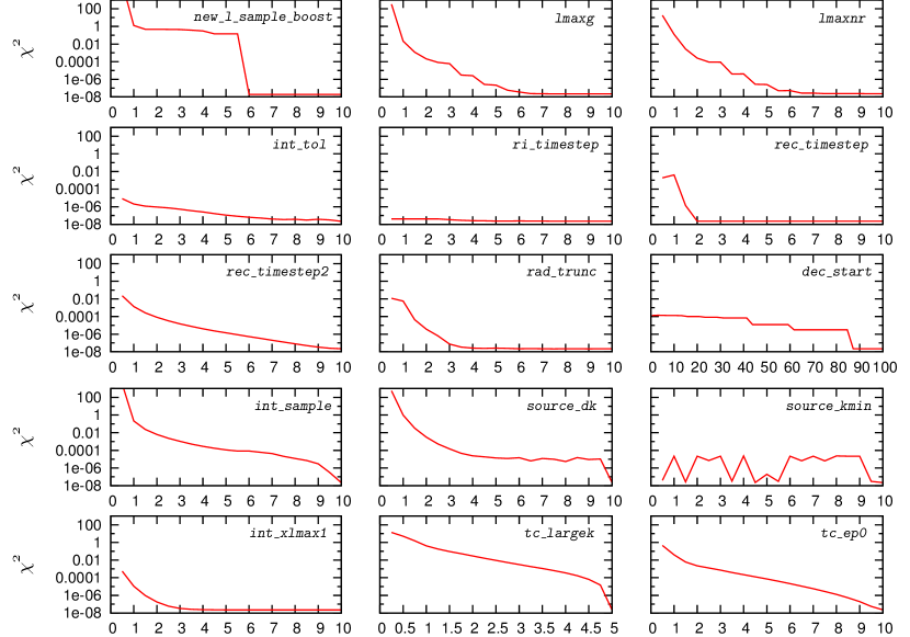
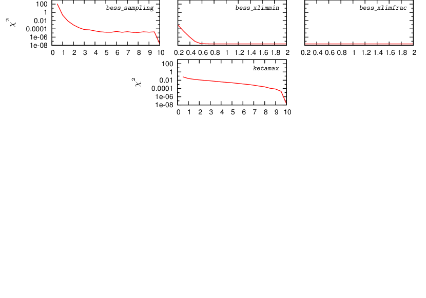
We show the results of the single parameter scans in Figure 1-2. From Figure 1 we can see that certain parameters (e.g., lmaxg, lmaxnr) are very well-behaved and reach a $\chi^{2}\sim 10^{-8}$ plateau well below the fiducial value. For these parameters it is reasonable to assume that picking even higher values would not have any appreciable effect on accuracy. A number of other parameters do not fully converge, and exhibit a step-like behaviour before reaching the fiducial value (e.g., int_sample, source_dk). It is likely that increasing their value beyond our fiducial maximum value would have an effect on the spectra. However, the graphs in Figure 1 nonetheless provide an order of magnitude estimate of the remaining error and one can use them as a guide to finding reasonable settings for the construction of the reference spectrum. Finally, the parameter source_kmin does not seem to converge at all and exhibits unstable behaviour, though its effect on overall accuracy is negligible.

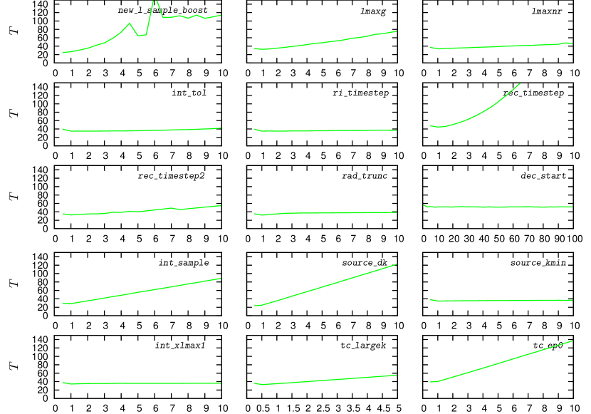
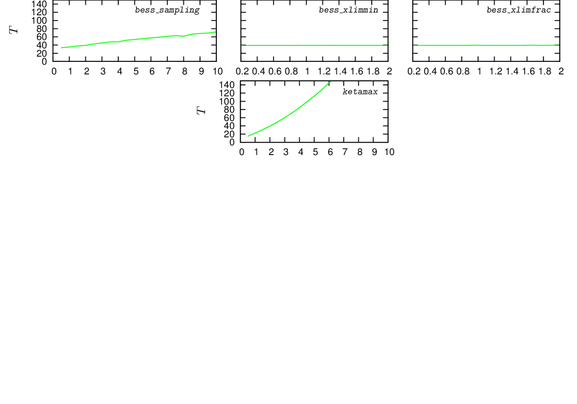
The parameter settings we chose for the reference spectrum are given in Table 4. The dominant contribution to any residual error of the reference spectrum will come from the parameter displaying the worst convergence – ketamax. Unfortunately, this parameter also has a strong impact on the computation time $T$ (see Figure 2), and memory requirements, precluding us from choosing a higher setting. We estimate the reference spectrum to be accurate to $\Delta\chi^{2}$ of order $10^{-2}$.

Table 4: Accuracy settings for the reference spectrum (plus three recommended example settings, see Section 3).

Parameter	Reference setting	Setting 1	Setting 2	Setting 3
new_l_sample_boost	6	1.77	1.60	2.00
lmaxg	6	7.39	2.02	2.05
lmaxnr	6	1.78	2.11	5.36
int_tol	6	2.07	1.53	5.86
ri_timestep	2	0.99	0.71	2.87
rec_timestep	3	0.50	0.50	0.75
rec_timestep2	10	1.85	1.14	2.44
rad_trunc	4	1.81	1.76	2.58
dec_start	100	2.35	35.76	5.05
int_sample	6	4.21	4.88	3.65
source_dk	4	3.10	2.84	2.72
source_kmin	1	5.86	2.50	5.23
int_xlmax1	4	1.20	1.00	2.16
tc_largek	5	2.44	2.33	1.90
tc_ep0	5	4.25	3.30	6.32
bess_sampling	3	3.02	2.53	4.00
bess_xlimmin	2	1.14	0.74	3.61
bess_xlimfrac	2	4.19	0.90	1.07
ketamax	3	1.32	0.96	0.56

Figure 1: These diagrams illustrate the dependence of accuracy on the settings of individual parameters. We plot $\chi^{2}$ as a function of parameter value. The fiducial reference data sets were generated with all parameters set to a value of 2, except for the one scanned, which is set to an extremely high value (100 for dec_start, 5 for tc_largek, and 10 for all other parameters). When setting the accuracy parameters to their fiducial values, we obtain a $\chi^{2}$ of order $10^{-8}$ instead of 0. This effect stems from a numerical rounding error when outputting the fiducial data set, and is small enough not to be of relevance to any of our conclusions.

Figure 2: These diagrams show the computation time $T$ (in seconds), varying the settings of all parameters individually while keeping all others fixed at a value of 2. The calculations were performed on a single core of a $2.40\rm{\ GHz}$ Intel T7700 CPU. The spikes for new_l_sample_boost, as well as the “bumps” at low settings of various other parameters are due to the fact that the Bessel functions were (re-)calculated at these points, adding a few seconds to the total time.

3 Optimising performance

Having constructed the reference spectra, we can now proceed to searching settings of the accuracy parameters which yield a result that lies as close as possible to the reference spectra, within a reasonable time of computation. To this end, we use a modified version of the Markov chain Monte Carlo code CosmoMC [15]. Major modifications include:

• we use the fiducial data set constructed from the reference spectra;

• we vary the accuracy parameters instead of the cosmological parameters (which are kept fixed at their fiducial values), taking top hat priors on all accuracy parameters (with lower limits at a value of 0.5 and upper limits large enough to not influence the results);

• instead of sampling from the usual posterior $\mathcal{P}$ (which is proportional to $\mathcal{L}\sim\exp[-\chi^{2}/2]$) itself, we sample a function $F(\mathcal{P})$, defined by

  $$F(\mathcal{P})=\left\{\begin{array}[]{c c l}0&\quad\mbox{if}&\mbox{$T>60\ \rm{s}$}\\ \mathcal{P}&\quad\mbox{if}&\mbox{$\mathcal{P}\geq 1$}\\ 5\ln{\left[\mathcal{P}\right]}+1&\quad\mbox{if}&\mbox{$\mathcal{P}<1$}\\ \end{array}\right.$$ (3.1)

  This function was chosen such that areas of parameter space leading to too long computation times are avoided, and that areas of parameter space giving $\chi^{2}\ll 1$ are better sampled.

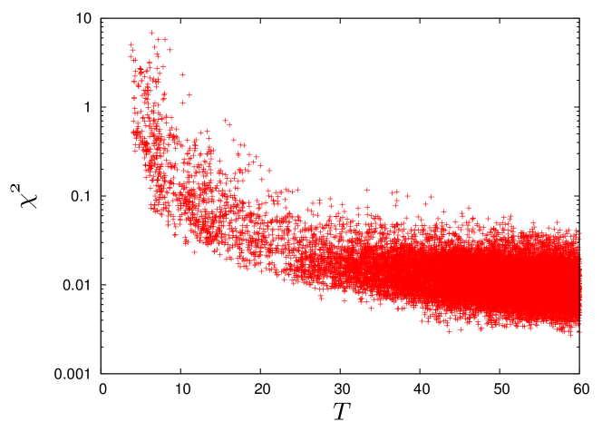
We generated $\sim\!\!20000$ sample settings in this way; a scatter plot of the samples in the $(\chi^{2},T)$-plane is presented in Figure 3, illustrating the strong correlation between accuracy and computation time. Which settings to use is a somewhat subjective decision and should be taken with one’s available computing power in mind. We list two sample settings in Table 4, taken from the samples of our Monte Carlo run: “Setting 1” corresponds to the best accuracy under the constraint that the computing time be less than 60 seconds, “Setting 2” gives the best accuracy for $T<30\ {\rm s}$, and “Setting 3” the best accuracy for $T<17.6\ {\rm s}$ (which is the computation time for the unmodified version of CAMB run at accuracy_level = 2). The performance of these settings is contrasted to CAMB’s default (accuracy_level = 1), and a high-accuracy setting of an unmodified version of CAMB (accuracy_level = 2) in Table 5.

Note that at the default settings, with a difference of $\Delta\chi^{2}$ to the reference spectra, parameter estimates could be biased by more than two standard deviations, in the worst case. For both Settings 1 and 2, on the other hand, the maximum possible bias would be less than 0.1 standard deviations ($\sim 0.13$ standard deviations for Setting 3), assuming Gaussian posterior distributions.

The results of the MCMC search confirm the tendencies observed in the single parameter scans of Figs. 1 and 2 regarding the impact of individual parameters on accuracy and speed; we find no evidence for significant cross-correlations between accuracy parameters.

Figure 3: Computation time versus $\chi^{2}$ for the $\sim 20000$ samples of our Monte Carlo run.

Table 5: Deviation from reference spectrum, given in terms of $\chi^{2}$, and computation time $T$, for the three example settings of Table 4, CAMB’s default settings ($\texttt{accuracy\_level}=1$) and $\texttt{accuracy\_level}=2$.

Setting	$\chi^{2}$	$T\cdot s^{-1}$
1	$2.7\cdot 10^{-3}$	59
2	$7.0\cdot 10^{-3}$	27
3	$1.6\cdot 10^{-2}$	17.4
$\texttt{accuracy\_level}=1$	5.8	2.7
$\texttt{accuracy\_level}=2$	0.5	17.6

4 Estimating the bias

As mentioned above, the $\chi^{2}$ for a given accuracy settings can be used to estimate the worst case bias on cosmological parameters. Nevertheless, we are also interested in how large a bias effect we can expect in the example case of the vanilla model. To this end, we performed an actual parameter estimation exercise using CosmoMC, for three cases:

• Using the same CAMB accuracy settings for generating the fiducial data as for the inference process – mimicking an analysis free of numerical errors.

• Using the reference data set and running CAMB at accuracy settings “2” from Table 4.

• Using the reference data set and running CAMB at its default settings.

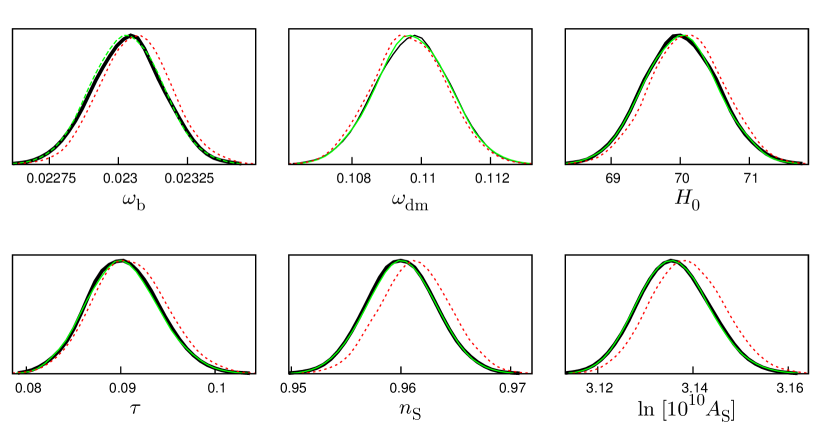
We generate 16 Markov chains, making sure the Gelman-Rubin convergence parameter $R-1$ [16] is smaller than $10^{-2}$ for all parameters considered. The results are plotted in Figure 4: as expected, there is no discernible bias between the results obtained with optimised settings and an error-free analysis. The expected bias for the default settings is rather mild, not exceeding a few tenths of the posterior standard deviations for the respective parameters, with $n_{\rm S}$ (40%) and $\ln\left[10^{10}A_{\rm S}\right]$ (43%) being the most affected.

Figure 4: Marginalised posterior probability densities of the cosmological parameters of the vanilla model. Thick black lines correspond to the exact results (using the same accuracy settings for the MCMC and for the fiducial data set), green lines are results obtained with the “Settings 2” column of Table 4 and the reference data set, and the red dotted lines represent the posteriors from the default accuracy settings of CosmoMC/CAMB and the reference data set.

5 Conclusions

To meet the challenge posed by ultra-precise future CMB experiments, the output of the Boltzmann codes used to calculate theoretical predictions for the CMB anisotropy spectra will have to meet stringent requirements in terms of numerical accuracy – a goal that comes at the cost of accordingly higher demand in computational resources. This tendency is partially mitigated by the increase in available computing power. Additionally, the use of efficient interpolation algorithms [17, 18, 19, 20] can significantly accelerate the process of parameter estimation from future data sets. Nonetheless, such methods still rely on the input of a full Boltzmann code, whose inherent numerical errors will be propagated to the interpolation codes.

We have performed a detailed analysis of the numerical accuracy of CAMB, provided an estimate of the residual numerical error of the output, and evaluated the possible impact on parameter estimates from planck data. For the present default accuracy settings of CAMB and simulated planck data, numerical errors can lead to a slight bias on estimates of the six free parameters of the $\Lambda$CDM model; though we cannot exclude the possibility of a more serious bias on parameters of extended models. However, by tweaking the settings of various internal parameters of CAMB it can be made sure that the bias on any parameter will not exceed 0.1 standard deviations. An example for suggested settings of the accuracy parameters is given in Table 4.

The results of this paper lead to an efficient and more accurate calculation of CMB angular power spectra, and should bring CAMB to a standard that will allow us to make the most out of upcoming planck data. We conclude that the contribution of numerical errors to the theoretical uncertainty of model predictions is well under control – the main challenges for more accurate calculations of CMB spectra will be of an astrophysical nature instead.

References

- [1] W. Hu, D. Scott, N. Sugiyama and M. J. White, Phys. Rev. D 52 (1995) 5498 [arXiv:astro-ph/9505043].
- [2] W. A. Fendt, J. Chluba, J. A. Rubino-Martin and B. D. Wandelt, arXiv:0807.2577 [astro-ph].
- [3] A. Lewis, J. Weller and R. Battye, Mon. Not. Roy. Astron. Soc. 373 (2006) 561 [arXiv:astro-ph/0606552].
- [4] U. Seljak, N. Sugiyama, M. J. White and M. Zaldarriaga, Phys. Rev. D 68 (2003) 083507 [arXiv:astro-ph/0306052].
- [5] [Planck Collaboration], arXiv:astro-ph/0604069.
- [6] E. Bertschinger, arXiv:astro-ph/9506070.
- [7] U. Seljak and M. Zaldarriaga, Astrophys. J. 469 (1996) 437 [arXiv:astro-ph/9603033].
- [8] A. Lewis, A. Challinor and A. Lasenby, Astrophys. J. 538 (2000) 473 [arXiv:astro-ph/9911177].
- [9] M. Doran, JCAP 0510 (2005) 011 [arXiv:astro-ph/0302138].
- [10] J. Dunkley et al. [WMAP Collaboration], arXiv:0803.0586 [astro-ph].
- [11] A. Lewis and A. Challinor, Phys. Rept. 429 (2006) 1 [arXiv:astro-ph/0601594].
- [12] L. Perotto, J. Lesgourgues, S. Hannestad, H. Tu and Y. Y. Y. Wong, JCAP 0610 (2006) 013 [arXiv:astro-ph/0606227].
- [13] J. Hamann and Y. Y. Y. Wong, JCAP 0803 (2008) 025 [arXiv:0709.4423 [astro-ph]].
- [14] S. Hamimeche and A. Lewis, Phys. Rev. D 77 (2008) 103013 [arXiv:0801.0554 [astro-ph]].
- [15] A. Lewis and S. Bridle, Phys. Rev. D 66 (2002) 103511 [arXiv:astro-ph/0205436].
- [16] A. Gelman and D. B. Rubin, Statist. Sci. 7 457-511
- [17] H. B. Sandvik, M. Tegmark, X. M. Wang and M. Zaldarriaga, Phys. Rev. D 69 (2004) 063005 [arXiv:astro-ph/0311544].
- [18] W. A. Fendt and B. D. Wandelt, Astrophys. J. 654 (2006) 2 [arXiv:astro-ph/0606709].
- [19] T. Auld, M. Bridges, M. P. Hobson and S. F. Gull, Mon. Not. Roy. Astron. Soc. Lett. 376 (2007) L11 [arXiv:astro-ph/0608174].
- [20] W. A. Fendt and B. D. Wandelt, arXiv:0712.0194 [astro-ph].