Maximal parabolic regularity for divergence operators including mixed boundary conditions

Abstract.

We show that elliptic second order operators $A$ of divergence type fulfill maximal parabolic regularity on distribution spaces, even if the underlying domain is highly non-smooth, the coefficients of $A$ are discontinuous and $A$ is complemented with mixed boundary conditions. Applications to quasilinear parabolic equations with non-smooth data are presented.

1. Introduction

It is known that divergence operators fulfill maximal parabolic regularity on $L^{p}$ spaces – even if the underlying domain is non-smooth, the coefficients are discontinuous and the boundary conditions are mixed, see [6] and also [59]. This provides a powerful tool for the treatment of linear and nonlinear parabolic equations in $L^{p}$ spaces, see [77, 24, 71, 59]. The only disadvantage of this concept is that the appearing Neumann conditions have to be homogeneous and that distributional right hand sides (e.g. surface densities) are not admissible. Confronted with these phenomena, it seems an adequate alternative to consider the equations in distribution spaces, what we will do in this paper. Pursuing this idea, one has, of course, to prove that the occurring elliptic operators satisfy parabolic regularity on those spaces in an appropriate sense.

In fact, we show that, under very mild conditions on the domain $\Omega$, the Dirichlet boundary part $\partial\Omega\setminus\Gamma$ and the coeffcient function, elliptic divergence operators with real $L^{\infty}$-coefficients satisfy maximal parabolic regularity on a huge variety of spaces, among which are Sobolev, Besov and Lizorkin-Triebel spaces, provided that the differentiability index is between $0$ and $-1$ (cf. Theorem 5.16). We consider this as the first main result of this work, also interesting in itself. Up to now, the only existing results for mixed boundary conditions in distribution spaces (apart from the Hilbert space situation) are, to our knowledge, that of Gröger [55] and the recent one of Griepentrog [51]. Concerning the Dirichlet case, compare [18] and references therein.

Having this first result at hand, the second aim of this work is the treatment of quasilinear parabolic equations of the formal type

$$\left\{\begin{aligned} \bigl{(}\mathcal{F}(u)\bigr{)}^{\prime}-\nabla\cdot\mathcal{G}(u)\mu\nabla u&=\mathcal{R}(t,u),\\ u(T_{0})&=u_{0},\end{aligned}\right.$$ (1.1)

combined with mixed, nonlinear boundary conditions:

$$\nu\cdot\mathcal{G}(u)\mu\nabla u+b(u)=g\text{ on }\Gamma\qquad\text{and}\qquad u=0\text{ on }\partial\Omega\setminus\Gamma.$$ (1.2)

Let us point out some ideas, which will give a certain guideline for the paper: Our analysis is based on a regularity result for the square root $(-\nabla\cdot\mu\nabla)^{1/2}$ on $L^{p}$ spaces. It has already been remarked in the introduction of [12] that estimates between $\|(-\nabla\cdot\mu\nabla)^{1/2}f\|_{p}$ and $\|\nabla f\|_{p}$ should provide powerful tools for the treatment of elliptic and parabolic problems involving divergence form operators. It seems, however, that this idea has not yet been developed to its full strength, cf. [35, Ch. 5].

Originally, our strategy for proving maximal parabolic regularity for divergence operators on $H^{-1,q}_{\Gamma}$ was to show an analog of the central result of [12], this time in case of mixed boundary conditions, namely that

$$\bigl{(}-\nabla\cdot\mu\nabla+1\bigr{)}^{-1/2}:L^{q}\to H^{1,q}_{\Gamma}$$ (1.3)

provides a topological isomorphism for suitable $q$. This would give the possibility of carrying over the maximal parabolic regularity, known for $L^{q}$, to the dual of $H^{1,q^{\prime}}_{\Gamma}$, because, roughly spoken, $(-\nabla\cdot\mu\nabla+1)^{-1/2}$ commutes with the corresponding parabolic solution operator. Unfortunately, we were only able to prove the continuity of (1.3) within the range $q\in[2,\infty[$, due to a result of Duong and $\rm M^{c}$Intosh [32], but did not succeed in proving the continuity of the inverse in general. Let us explicitely mention that the proof of the isomorphism property of (1.3) would be a great achievement. In particular, this would allow here to avoid the localization procedure we had to introduce in Section 5 in order to prove maximal parabolic regularity, and to generalize our results to higher dimensions. The isomorphism property is known for the Hilbert space case $L^{2}$ (see [13]) in case of mixed boundary conditions and even complex coefficients, but the proof fundamentally rests on the Hilbert space structure, so that we do not see a possibility of directly generalizing this to the $L^{p}$ case.

It turns out, however, that (1.3) provides a topological isomorphism, if $\Omega\cup\Gamma$ is the image under a volume-preserving and bi-Lipschitz mapping of one of Gröger’s model sets [53], describing the geometric configuration in neighborhoods of boundary points of $\Omega$. Thus, in these cases one may carry over the maximal parabolic regularity from $L^{q}$ to $H^{-1,q}_{\Gamma}.$ Knowing this, we localize the linear parabolic problem, use the ’local’ maximal parabolic information and interpret this again in the global context at the end. Interpolation with the $L^{p}$ result then yields maximal parabolic regularity on the corresponding interpolation spaces.

Let us explicitely mention that the concept of Gröger’s regular sets, where the domain itself is a Lipschitz domain, seems adequate to us, because it covers many realistic geometries that fail to be domains with Lipschitz boundary. The price one has to pay is that the problem of optimal elliptic regularity becomes much more delicate and, additionally, trace theorems for this situation are scarcely to be found in the literature.

The strategy for proving that (1.1), (1.2) admit a unique local solution is as follows. We reformulate (1.1) into a usual quasilinear equation, where the time derivative directly affects the unknown function. Assuming additionally that the elliptic operator $-\nabla\cdot\mu\nabla+1:H^{1,q}_{\Gamma}\to H^{-1,q}_{\Gamma}$ provides a topological isomorphism for a $q$ larger than the space dimension $d$, the existence and uniqueness results for abstract quasilinear equations of Prüss (see [77], see also [24]) apply to the resulting quasilinear parabolic equation. The detailed discussion how to assure all requirements of [77], including the adequate choice of the Banach space, is presented in Section 6. The crucial point is that the linear elliptic operator which corresponds to the initial value satisfies maximal parabolic regularity, which has been proved before. Let us further emphasize that the presented setting allows for coefficient functions that really jump at hetero interfaces of the material and permits mixed boundary conditions, as well as domains which do not possess a Lipschitz boundary, see Section 7. It is well known that this is required when modelling real world problems, see e.g. [83, 20] for problems from thermodynamics or [38, 16] concerning biological models. Last but not least, heterostructures are the determining features of many fundamental effects in semiconductors, see for instance [80, 14, 63].

One further advantage is that nonlinear, nonlocal boundary conditions are admissible in our concept, despite the fact that the data is highly non-smooth, compare [2]. The calculus of maximal parabolic $L^{s}(\left]T_{0},T\right[;X)$ regularity is preferable to the concept of Hölder continuity in time, because it allows for reaction terms $\mathcal{R}$ which discontinously depend on time. This is important in many examples (see [88, 58, 65]), in particular in the control theory of parabolic equations. Alternatively, the reader should think e.g. of a manufacturing process for semiconductors, where light is switched on/off at a sharp time point and, of course, parameters in the chemical process then change abruptly. It is remarkable that, nevertheless, the solution is Hölder continuous simultaneously in space and time, see Corollary 6.16 below.

We finish these considerations by looking at the special case of semilinear problems. It turns out that here satisfactory results may be achieved even without the additional continuity condition on $-\nabla\cdot\mu\nabla+1$ mentioned above, see Corollary 6.17.

In Section 7 we give examples for geometries, Dirichlet boundary parts and coefficients in three dimensions for which our additional supposition, the isomorphy $-\nabla\cdot\mu\nabla+1:H^{1,q}_{\Gamma}\to H^{-1,q}_{\Gamma}$ really holds for a $q>d$. In Subsection 7.3 we take a closer look at the special geometry of two crossing beams, which provides a geometrically easy example of a domain $\Omega$ that does not have a Lipschitz boundary and thus cannot be treated by former theories, but which is covered by our results.

Finally, some concluding remarks are given in Section 8.

2. Notation and general assumptions

Throughout this article the following assumptions are valid.

• $\Omega\subseteq{\mathbb{R}}^{d}$ is a bounded Lipschitz domain and $\Gamma$ is an open subset of $\partial\Omega$.

• The coefficient function $\mu$ is a Lebesgue measurable, bounded function on $\Omega$ taking its values in the set of real, symmetric, positive definite $d\times d$ matrices, satisfying the usual ellipticity condition.

Remark 2.1.

Concerning the notions ’Lipschitz domain’ and ’domain with Lipschitz boundary’ (synonymous: strongly Lipschitz domain) we follow the terminology of Grisvard [52], see also [70].

For $\varsigma\in\left]0,1\right]$ and $1<q<\infty$ we define $H^{\varsigma,q}_{\Gamma}(\Omega)$ as the closure of

$$C^{\infty}_{\Gamma}(\Omega):=\{\psi|_{\Omega}:\psi\in C^{\infty}({\mathbb{R}}^{d}),\;\operatorname{supp}(\psi)\cap(\partial\Omega\setminus\Gamma)=\emptyset\}$$ (2.1)

in the Sobolev space $H^{\varsigma,q}(\Omega)$. Of course, if $\Gamma=\emptyset$, then $H_{\Gamma}^{\varsigma,q}(\Omega)=H_{0}^{\varsigma,q}(\Omega)$ and if $\Gamma=\partial\Omega$, then $H_{\Gamma}^{\varsigma,q}(\Omega)=H^{\varsigma,q}(\Omega)$. This last point follows from the fact that $\Omega$, as a Lipschitz domain, admits a continuous extension operator from $H^{1,q}(\Omega)$ into $H^{1,q}({\mathbb{R}}^{d})$, see [45, Thm. 3.10]. Thus, the set $C^{\infty}(\Omega):=\{\psi|_{\Omega}:\psi\in C^{\infty}({\mathbb{R}}^{d})\}$ is dense in $H^{1,q}(\Omega)$. Concerning the dual of $H^{\varsigma,q}_{\Gamma}(\Omega)$, we have to distinguish between the space of linear and the space of anti-linear forms on this space. We define $H^{-\varsigma,q}_{\Gamma}(\Omega)$ as the space of continuous, linear forms on $H^{\varsigma,q^{\prime}}_{\Gamma}(\Omega)$ and $\breve{H}^{-\varsigma,q}_{\Gamma}(\Omega)$ as the space of anti-linear forms on $H^{\varsigma,q^{\prime}}_{\Gamma}(\Omega)$ if $1/q+1/q^{\prime}=1$. Note that $L^{p}$ spaces may be viewed as part of $\breve{H}^{-\varsigma,q}_{\Gamma}$ for suitable $\varsigma,q$ via the identification of an element $f\in L^{p}$ with the anti-linear form $H^{\varsigma,q^{\prime}}_{\Gamma}\ni\psi\mapsto\int_{\Omega}f\overline{\psi}\,{\mathrm{d}}\mathrm{x}$.

If misunderstandings are not to be expected, we drop the $\Omega$ in the notation of spaces, i.e. function spaces without an explicitely given domain are to be understood as function spaces on $\Omega$.

By $K$ we denote the open unit cube in ${\mathbb{R}}^{d}$, by $K_{-}$ the lower half cube $K\cap\{\mathrm{x}\,:\,x_{d}<0\}$, by $\Sigma={K}\cap\{\mathrm{x}\,:\,x_{d}=0\}$ the upper plate of $K_{-}$ and by $\Sigma_{0}$ the left half of $\Sigma$, i.e. $\Sigma_{0}=\Sigma\cap\{\mathrm{x}\,:\,x_{d-1}<0\}$.

As in the preceding paragraph, we will throughout the paper use $\mathrm{x},\mathrm{y},\dots$ for vectors in ${\mathbb{R}}^{d}$, whereas the components of $\mathrm{x}$ will be denoted by italics $x_{1},x_{2},\dots,x_{d}$ or in three dimensions also by $x,y,z$.

If $B$ is a closed operator on a Banach space $X$, then we denote by $dom_{X}(B)$ the domain of this operator. $\mathcal{L}(X,Y)$ denotes the space of linear, continuous operators from $X$ into $Y$; if $X=Y$, then we abbreviate $\mathcal{L}(X)$. Furthermore, we will write $\langle\cdot,\cdot\rangle_{X^{\prime}}$ for the dual pairing of elements of $X$ and the space $X^{\prime}$ of anti-linear forms on $X$.

Finally, the letter $c$ denotes a generic constant, not always of the same value.

3. Preliminaries

In this section we will properly define the elliptic divergence operator and afterwards collect properties of the $L^{p}$ realizations of this operator which will be needed in the subsequent chapters. First of all we establish the following extension property for function spaces on Lipschitz domains, which will be used in the sequel.

Proposition 3.1.

There is a continuous extension operator $\mathrm{Ext}:L^{1}(\Omega)\to L^{1}({\mathbb{R}}^{d})$, whose restriction to any space $H^{1,q}(\Omega)$ ($q\in\left]1,\infty\right[$) maps this space continuously into $H^{1,q}({\mathbb{R}}^{d})$. Moreover, $\mathrm{Ext}$ maps $L^{p}(\Omega)$ continuously into $L^{p}({\mathbb{R}}^{d})$ for $p\in\left]1,\infty\right]$.

Proof.

The assertion is proved for the spaces $H^{1,q}$ in [45, Thm. 3.10] see also [70, Ch. 1.1.16]. Inspecting the corresponding proofs (which are given via localization, Lipschitz diffeomorphism and symmetric reflection) one easily recognizes that the extension mapping at the same time continuously extends the $L^{p}$ spaces. ∎

Let us introduce an assumption on $\Omega$ and $\Gamma$ which will define the geometrical framework relevant for us in the sequel.

Assumption 3.2.

• For any point $\mathrm{x}\in\partial\Omega$ there is an open neighborhood $\Upsilon_{\mathrm{x}}$ of $\mathrm{x}$ and a bi-Lipschitz mapping $\phi_{\mathrm{x}}$ from $\Upsilon_{\mathrm{x}}$ into ${\mathbb{R}}^{d}$, such that $\phi_{\mathrm{x}}(\mathrm{x})=0$ and $\phi_{\mathrm{x}}\bigl{(}(\Omega\cup\Gamma)\cap\Upsilon_{\mathrm{x}}\bigr{)}=\alpha K_{-}$ or $\alpha(K_{-}\cup\Sigma)$ or $\alpha(K_{-}\cup\Sigma_{0})$ for some positive $\alpha=\alpha(\mathrm{x})$.

• Each mapping $\phi_{\mathrm{x}}$ is, in addition, volume-preserving.

Remark 3.3.

Assumption 3.2 a) exactly characterizes Gröger’s regular sets, introduced in his pioneering paper [53]. Note that the additional property ’volume-preserving’ also has been required in several contexts (see [48] and [55]).

It is not hard to see that every Lipschitz domain and also its closure is regular in the sense of Gröger, the corresponding model sets are then $K_{-}$ or $K_{-}\cup\Sigma$, respectively, see [52, Ch 1.2]. A simplifying topological characterization of Gröger’s regular sets for $d=2$ and $d=3$ will be given in Section 8.

In particular, all domains with Lipschitz boundary (strongly Lipschitz domains) satisfy Assumption 3.2: if, after a shift and an orthogonal transformation, the domain lies locally beyond a graph of a Lipschitz function $\psi$, then one can define $\phi(x_{1},\ldots,x_{d})=(x_{1}-\psi(x_{2},\ldots,x_{d}),x_{2},\ldots,x_{d})$. Obviously, the mapping $\phi$ is then bi-Lipschitz and the determinant of its Jacobian is identically $1$. For further examples see Section 7.

Next we have to introduce a boundary measure on $\partial\Omega$. Since in our context $\Omega$ is not necessarily a domain with Lipschitz boundary, this is not canonic. Let, according to the definition of a Lipschitz domain, for every point $\mathrm{x}\in\partial\Omega$ an open neighborhood $\Upsilon_{\mathrm{x}}$ of $\mathrm{x}$ and a bi-Lipschitz function $\phi_{\mathrm{x}}:\Upsilon_{\mathrm{x}}\to{\mathbb{R}}^{d}$ be given, which satisfy $\phi_{\mathrm{x}}(\Upsilon_{\mathrm{x}}\cap\Omega)=K_{-}$, $\phi_{\mathrm{x}}(\Upsilon_{\mathrm{x}}\cap\partial\Omega)=\Sigma$ and $\phi_{\mathrm{x}}(\mathrm{x})=\mathrm{0}$. Let $\Upsilon_{\mathrm{x}_{1}},\ldots,\Upsilon_{\mathrm{x}_{l}}$ be a finite subcovering of $\partial\Omega$. Define on $\partial\Omega\cap\Upsilon_{\mathrm{x}_{j}}$ the measure $\sigma_{j}$ as the $\phi_{\mathrm{x}_{j}}^{-1}$-image of the $(d-1)$-dimensional Lebesgue measure on $\Sigma$. Clearly, this measure is a positive, bounded Radon measure. Finally, define the measure $\sigma$ on $\partial\Omega$ by

$$\int_{\partial\Omega}f\,d\sigma:=\sum_{j=1}^{l}\int_{\partial\Omega\cap\Upsilon_{\mathrm{x}_{j}}}f\,d\sigma_{j},\quad f\in C(\partial\Omega).$$

Clearly, $\sigma$ also is a bounded, positive Radon measure. Furthermore, it is not hard to see that the measure $\sigma$ – simultaneously viewed as a measure on ${\mathbb{R}}^{d}$ – satisfies

$$\sup_{\mathrm{x}\in{\mathbb{R}}^{d}}\sup_{r\in\left]0,1\right[}\sigma(B(\mathrm{x},r))r^{1-d}<\infty,$$

where, here and in the sequel, $B(\mathrm{x},r)$ denotes the ball centered at $\mathrm{x}$ with radius $r$, compare [61, Ch. II.1], in particular Example 1 there.

Later we will repeatedly need the following interpolation results from [48].

Proposition 3.4.

Let $\Omega$ and $\Gamma$ satisfy Assumption 3.2 a) and let $\theta\in\left]0,1\right[$.

1. Then for $q_{0},q_{1}\in\left]1,\infty\right[$ and $\frac{1}{q}=\frac{1-\theta}{q_{0}}+\frac{\theta}{q_{1}}$ one has

   $$H_{\Gamma}^{\theta,q} =\bigl{[}L^{q_{0}},H_{\Gamma}^{1,q_{1}}\bigr{]}_{\theta},\quad \text{if }\theta\neq\frac{1}{q},$$ (3.1)

   $$H_{\Gamma}^{-\theta,q} =\bigl{[}L^{q_{0}},H_{\Gamma}^{-1,q_{1}}\bigr{]}_{\theta}\quad \text{if }\theta\neq 1-\frac{1}{q}$$ (3.2)

   and

   $$H^{\pm 1,q}_{\Gamma} =\bigl{[}H^{\pm 1,q_{0}}_{\Gamma},H^{\pm 1,q_{1}}_{\Gamma}]_{\theta}.$$ (3.3)

2. If additionally Assumption 3.2 b) is fulfilled and $\frac{1}{q}\neq\theta\neq 1-\frac{1}{q}$, then

   $$H_{\Gamma}^{\pm\theta,q}=\bigl{[}H_{\Gamma}^{-1,q},H_{\Gamma}^{1,q}\bigr{]}_{\frac{1\pm\theta}{2}}.$$ (3.4)

Corollary 3.5.

Under the same assumptions as for (3.3) one has

$$\breve{H}^{-1,q}_{\Gamma}=\bigl{[}\breve{H}^{-1,q_{0}}_{\Gamma},\breve{H}^{-1,q_{1}}_{\Gamma}]_{\theta}.$$ (3.5)

Proof.

(3.5) may be deduced from (3.3) by means of the retraction/coretraction theorem (see [85, Ch. 1.2.4]), where the coretraction is the mapping which assigns to $f\in\breve{H}^{-1,r}_{\Gamma}$ the linear form $H^{1,r^{\prime}}_{\Gamma}\ni\psi\to\langle f,\overline{\psi}\rangle_{\breve{H}^{-1,r}_{\Gamma}}$. ∎

Having this at hand, we can prove the following trace theorem.

Theorem 3.6.

Assume $q\in\left]1,\infty\right[$ and $\theta\in\bigl{]}\frac{1}{q},1\bigr{[}$. Let $\Pi$ be a Lipschitz hypersurface in $\overline{\Omega}$ and let $\varpi$ be any measure on $\Pi$ which satisfies

$$\sup_{\mathrm{x}\in{\mathbb{R}}^{d}}\sup_{r\in\left]0,1\right[}\varpi(B(\mathrm{x},r))r^{1-d}<\infty.$$

Then the trace operator $\mathrm{Tr}$ from $H^{\theta,q}(\Omega)$ to $L^{q}(\Pi,\varpi)$ is continuous.

Proof.

Since $\Omega$ is an extension domain for $H^{1,q}$ and $L^{q}$ simultaneously, one has the inequality

$$\|u|_{\Pi}\|_{L^{q}(\Pi,\varpi)}=\|u\|_{L^{q}(\overline{\Omega},\varpi)}\leq c\|u\|_{H^{1,q}(\Omega)}^{1/q}\|u\|_{L^{q}(\Omega)}^{1-1/q}\leq c\|u\|_{H^{1,q}(\Omega)},\quad u\in H^{1,q}(\Omega),$$ (3.6)

for $q\in\left]1,\infty\right[$, see [70, Ch. 1.4.7]. But due to a general interpolation principle (see [15, Ch. 5, Prop. 2.10]) this yields a continuous mapping

$$\bigl{(}L^{q}(\Omega),H^{1,q}(\Omega)\bigr{)}_{\frac{1}{q},1}\ni u\mapsto u|_{\Pi}\in L^{q}(\Pi,\varpi).$$ (3.7)

Since $\Omega$ is a Lipschitz domain, (3.1) in particular yields the equality $H^{\theta,q}(\Omega)=[L^{q}(\Omega),H^{1,q}(\Omega)]_{\theta}$ in view of $\theta>1/q$. Thus, we have the continuous embedding

$$H^{\theta,q}(\Omega)=\bigl{[}L^{q}(\Omega),H^{1,q}(\Omega)\bigr{]}_{\theta}\hookrightarrow\bigl{(}L^{q}(\Omega),H^{1,q}(\Omega)\bigr{)}_{\frac{1}{q},1},$$

see [85, Ch. 1.10.3, Thm. 1 and Ch. 1.3.3]. This, together with (3.7), proves the theorem. ∎

We define the operator $A:H^{1,2}_{\Gamma}\to\breve{H}^{-1,2}_{\Gamma}$ by

$$\langle A\psi,\varphi\rangle_{\breve{H}^{-1,2}_{\Gamma}}:=\int_{\Omega}\mu\nabla\psi\cdot\nabla\overline{\varphi}\;{\mathrm{d}}\mathrm{x}+\int_{\Gamma}\varkappa\,\psi\,\overline{\varphi}\;{\mathrm{d}}\sigma,\quad\psi,\varphi\in H^{1,2}_{\Gamma},$$ (3.8)

where $\varkappa\in L^{\infty}(\Gamma,{\mathrm{d}}\sigma)$. Note that in view of (3.6) the form in (3.8) is well defined.

In the special case $\varkappa=0$, we write more suggestively $-\nabla\cdot\mu\nabla$ instead of $A$.

The $L^{2}$ realization of $A$, i.e. the maximal restriction of $A$ to the space $L^{2}$, we denote by the same symbol $A$; clearly this is identical with the operator which is induced by the form on the right hand side of (3.8). If $B$ is a selfadjoint operator on $L^{2}$, then by the $L^{p}$ realization of $B$ we mean its restriction to $L^{p}$ if $p>2$ and the $L^{p}$ closure of $B$ if $p\in\left[1,2\right[$.

We decided not to use different symbols for all these (and lateron also other) realizations of our operators in this paper, since we think that the gain in exacteness would be largely outweighed by the resulting complexity of notation. Naturally, this means that we have to pay attention to domains even more thoroughly.

Remark 3.7.

Following [75, Ch. 1.4.2] (see also [17, Ch. 1]), we did not define $A$ as an operator with values in the space of linear forms on $H^{1,2}_{\Gamma}$, but in the space of anti-linear forms. This guarantees that the restriction of this operator to $L^{2}$ equals the usual selfadjoint operator that is induced by the sesquilinear form in (3.8), which is crucial for our analysis. In this spirit, the duality between $\breve{H}^{-1,q}_{\Gamma}$ and $H^{1,q^{\prime}}_{\Gamma}$ is to be considered as the extended $L^{2}$ duality $L^{2}\times L^{2}\ni(\psi,\varphi)\to\int_{\Omega}\psi\overline{\varphi}\;d\mathrm{x}$, where $L^{2}$ acts as the set of anti-linear forms on itself. Especially, all occurring adjoint operators are to be understood with respect to this dual pairing.

First, we collect some basic facts on $A$.

Proposition 3.8.

1. $\nabla\cdot\mu\nabla$ generates an analytic semigroup on $\breve{H}^{-1,2}_{\Gamma}$.

2. $-\nabla\cdot\mu\nabla$ is selfadjoint on $L^{2}$ and bounded by $0$ from below. The restriction of $-A$ to $L^{2}$ is densely defined and generates an analytic semigroup there.

3. If $\lambda>0$ then the operator $(-\nabla\cdot\mu\nabla+\lambda)^{1/2}:H^{1,2}_{\Gamma}\to L^{2}$ provides a topological isomorphism; in other words: the domain of $(-\nabla\cdot\mu\nabla+\lambda)^{1/2}$ on $L^{2}$ is the form domain $H^{1,2}_{\Gamma}$.

4. The form domain $H^{1,2}_{\Gamma}$ is invariant under multiplication with functions from $H^{1,q}$, if $q>d$.

5. Assume $\varkappa\geq 0$. Then, under Assumption 3.2 a), for all $p\in\left]1,\infty\right[$ the operator $-A$ generates a semigroup of contractions on $L^{p}$. Additionally, it satisfies

   $$\|(A+\lambda)^{-1}\|_{\mathcal{L}(L^{p})}\leq\frac{c}{|\lambda|},\quad\operatorname{Re}\lambda\geq 0.$$

6. Under Assumption 3.2 a) $dom_{\breve{H}^{-1,q}_{\Gamma}}(-\nabla\cdot\mu\nabla)$ embeds compactly into $\breve{H}^{-1,q}_{\Gamma}$ for every $q\in[2,\infty[$, i.e. the resolvent of $(-\nabla\cdot\mu\nabla)$ is compact on $\breve{H}^{-1,q}_{\Gamma}$.

Proof.

1. is proved in [75, Thm. 1.55], see also [54].

2. The first assertion follows from a classical representation theorem for forms, see [64, Ch. VI.2.1]. Secondly, one verifies that the form $H^{1,2}_{\Gamma}\ni\psi\mapsto\int_{\Gamma}\varkappa|\psi|^{2}\,{\mathrm{d}}\sigma$ is form subordinated to the – positive – form $H^{1,2}_{\Gamma}\ni\psi\mapsto\int_{\Omega}\nabla\psi\cdot\mu\nabla\overline{\psi}+\psi\overline{\psi}\;{\mathrm{d}}\mathrm{x}$ with arbitrarily small relative bound. In fact, thanks to (3.6),

   $$\biggl{|}\int_{\Gamma}\varkappa|\psi|^{2}{\mathrm{d}}\sigma\biggr{|} \leq\|\varkappa\|_{L^{\infty}(\Gamma)}\|\psi\|_{L^{2}(\partial\Omega)}^{2}\leq\|\varkappa\|_{L^{\infty}(\Gamma)}\|\psi\|_{H^{1,2}_{\Gamma}(\Omega)}\|\psi\|_{L^{2}(\Omega)}$$

   $$\leq\varepsilon\|\psi\|^{2}_{H^{1,2}_{\Gamma}(\Omega)}+\frac{1}{\varepsilon}\|\varkappa\|^{2}_{L^{\infty}(\Gamma)}\|\psi\|^{2}_{L^{2}(\Omega)}.$$

   Thus, the form (3.8) is also closed on $H^{1,2}_{\Gamma}$ and sectorial. Moreover, the operator $-A$ generates an analytic semigroup by the representation theorem for sectorial forms, see also [64, Ch. VI.2.1].

3. This follows from the second representation theorem of forms (see [64, Ch. VI.2.6]), applied to the operator $-\nabla\cdot\mu\nabla+\lambda$.

4. First, for $u\in C^{\infty}_{\Gamma}$ and $v\in C^{\infty}$ the product $uv$ is obviously in $C^{\infty}_{\Gamma}\subseteq H^{1,2}_{\Gamma}$. But, by definition of $H^{1,2}_{\Gamma}$, the set $C^{\infty}_{\Gamma}$ (see (2.1)) is dense in $H^{1,2}_{\Gamma}$ and $C^{\infty}$ is dense in $H^{1,q}$. Thus, the assertion is implied by the continuity of the mapping

   $$H^{1,2}_{\Gamma}\times H^{1,q}\ni(u,v)\mapsto uv\in H^{1,2},$$

   because $H^{1,2}_{\Gamma}$ is closed in $H^{1,2}$.

5. This is proved in [49, Thm. 4.11, Thm. 5.2].

6. The operator $(-\nabla\cdot\mu\nabla+1)^{-1}$ has the following – continuous – mapping properties

   $$(-\nabla\cdot\mu\nabla+1)^{-1}:\breve{H}^{-1,2}_{\Gamma}\to H^{1,2}_{\Gamma}\hookrightarrow L^{2}$$ (3.9)

   and

   $$(-\nabla\cdot\mu\nabla+1)^{-1}:\breve{H}^{-1,q}_{\Gamma}\to L^{\infty}\hookrightarrow L^{d+1}\quad\text{for }q\geq d+1$$ (3.10)

   (see [50]). This shows that the resolvent is compact for $q=2$ and for $q\geq d+1$. If one takes in (3.10) $q=d+1$ and interpolates between (3.9) and (3.10), one obtains a continuous mapping $(-\nabla\cdot\mu\nabla+1)^{-1}:\breve{H}^{-1,q}_{\Gamma}\to L^{q}$ for every $q\in\left]2,d+1\right[$, see Corollary 3.5. ∎

One essential instrument for our subsequent considerations are (upper) Gaussian estimates.

Theorem 3.9.

The semigroup generated by $\nabla\cdot\mu\nabla$ in $L^{2}$ satisfies upper Gaussian estimates, precisely:

$$(\operatorname{e}^{t\nabla\cdot\mu\nabla}f)(\mathrm{x})=\int_{\Omega}K_{t}(\mathrm{x},\mathrm{y})f(\mathrm{y})\;{\mathrm{d}}\mathrm{y},\quad\mathrm{x}\in\Omega,\;f\in L^{2},$$

for some measurable function $K_{t}:\Omega\times\Omega\to{\mathbb{R}}_{+}$ and for all $\varepsilon>0$ there exist constants $c,b>0$, such that

$$0\leq K_{t}(\mathrm{x},\mathrm{y})\leq\frac{c}{t^{d/2}}\;\operatorname{e}^{-b\frac{|\mathrm{x}-\mathrm{y}|^{2}}{t}}\operatorname{e}^{\varepsilon t},\quad t>0,\;a.a.\;\mathrm{x},\mathrm{y}\in\Omega.$$ (3.11)

This follows from the following simplified version of Theorem 6.10 in [75] (see also [7]).

Proposition 3.10 (Ouhabaz).

Assume that $-\nabla\cdot\omega\nabla$, with $\omega\in L^{\infty}(\Omega;{\mathcal{L}}({\mathbb{R}}^{d}))$ uniformly elliptic, is defined on the form domain $V\subseteq H^{1,2}$ that satisfies

1. $V$ is closed in $H^{1,2}$,

2. $H^{1,2}_{0}\subseteq V$,

3. $V$ has the $L^{1}$-$H^{1,2}$ extension property,

4. $u\in V$ implies $\operatorname{sign}(u)\inf(1,|u|)\in V$, where $\operatorname{sign}(u)=u/|u|$ if $u\neq 0$ and $\operatorname{sign}(u)=0$ else.

5. $u\in V$ implies $\operatorname{e}^{\psi}u\in V$ for every $\psi\in C^{\infty}({\mathbb{R}}^{d})$, such that $\psi$ and $|\nabla\psi|$ are bounded in ${\mathbb{R}}^{d}$.

Then $\operatorname{e}^{t\nabla\cdot\omega\nabla}$ satisfies an upper Gaussian estimate as in (3.11).

Proof of Theorem 3.9.

We have to verify conditions a) – e) from Proposition 3.10 for $V=H^{1,2}_{\Gamma}$. a) and b) are obvious. For c) see Proposition 3.1 and d) is covered by [75, Proposition 4.11]. Finally, e) follows from Proposition 3.8 iv). ∎

Another notion in our considerations will be the bounded holomorphic functional calculus that we want to introduce briefly. Let $X$ be a Banach space and $-B$ the generator of a bounded analytic semigroup on $X$. Denoting, for $\kappa\in\left]0,\pi\right]$,

$$\Sigma_{\kappa}:=\{z\in{\mathbb{C}}\setminus\{0\}:|\arg(z)|<\kappa\},$$

we then have for some $\theta\in\left]0,\pi/2\right[$

$$\sigma(B)\subseteq\Sigma_{\theta}\cup\{0\}\quad\text{and}\quad\|R(\lambda,B)\|_{{\mathcal{L}}(X)}\leq\frac{M}{|\lambda|},\quad\lambda\in{\mathbb{C}}\setminus\overline{\Sigma_{\theta}}.$$

Following [73] (see also [27]), for any angle $\kappa\in\left]0,\pi\right]$ we define the function spaces

$$\mathcal{H}^{\infty}(\Sigma_{\kappa}) :=\{\psi:\Sigma_{\kappa}\to{\mathbb{C}},\text{ holomorphic and bounded}\}\quad\text{and}$$

$$\mathcal{H}^{\infty}_{0}(\Sigma_{\kappa}) :=\bigl{\{}\psi\in\mathcal{H}^{\infty}(\Sigma_{\kappa}):\text{ there exist }C,\varepsilon>0\text{ s.t. }|\psi(z)|\leq C\frac{|z|^{\varepsilon}}{(1+|z|)^{2\varepsilon}}\bigr{\}},$$

both equipped with the norm $\|\psi\|_{\mathcal{H}^{\infty}_{\kappa}}:=\sup_{z\in\Sigma_{\kappa}}|\psi(z)|$. Then for $\psi\in\mathcal{H}^{\infty}_{0}(\Sigma_{\kappa})$ with $\kappa>\theta$, we may compute $\psi(B)$, using the Cauchy integral formula

$$\psi(B)=\frac{1}{2\pi i}\int_{\angle}\psi(z)R(z,B)\;{\mathrm{d}}z,$$

where the path $\angle$ is given by the two rays $t\operatorname{e}^{\pm i\varphi}$, $t>0$, for some $\theta<\varphi<\kappa$. Note that this integral is absolutely convergent in ${\mathcal{L}}(X)$. We now say that $B$ has a bounded $\mathcal{H}^{\infty}$-calculus, if there is a constant $C\geq 0$, such that

$$\|\psi(B)\|_{{\mathcal{L}}(X)}\leq C\|\psi\|_{\mathcal{H}^{\infty}_{\kappa}},\quad\psi\in\mathcal{H}^{\infty}_{0}(\Sigma_{\kappa}),$$

for some $\kappa>\theta$. The infimum of all angles $\kappa$, for which this holds, is called the $\mathcal{H}^{\infty}$-angle $\varphi_{B}^{\infty}$ of $B$.

If $B$ admits a bounded $\mathcal{H}^{\infty}$-calculus for some $\kappa>\theta$, then the mapping $\mathcal{H}^{\infty}_{0}(\Sigma_{\kappa})\ni\psi\mapsto\psi(B)\in{\mathcal{L}}(X)$ can be extended uniquely to an algebra homomorphism between $\mathcal{H}^{\infty}(\Sigma_{\kappa})$ and ${\mathcal{L}}(X)$.

Proposition 3.11.

Let $\partial\Omega\setminus\Gamma$ have nonzero boundary measure. Then the following assertions hold for every $p\in\left]1,\infty\right[$.

1. For sufficiently small $\gamma>0$, the operator $-\nabla\cdot\mu\nabla-\gamma$ has a bounded $\mathcal{H}^{\infty}$-calculus on $L^{p}$ with $\mathcal{H}^{\infty}$-angle $\varphi^{\infty}_{-\nabla\cdot\mu\nabla-\gamma}=0$.

2. The set $\{(-\nabla\cdot\mu\nabla)^{is}:s\in{\mathbb{R}}\}$ forms a strongly continuous group on $L^{p}$ admitting the estimate

   $$\|(-\nabla\cdot\mu\nabla)^{is}\|_{\mathcal{L}(L^{p})}\leq c_{p}\operatorname{e}^{|s|\vartheta},\quad s\in{\mathbb{R}},$$

   with $0\leq\vartheta<\pi/2$.

Proof.

Since the boundary measure of $\partial\Omega\setminus\Gamma$ is nonzero, the operator $-\nabla\cdot\mu\nabla$ is continuously invertible in $L^{2}$, i.e. $0$ does not belong to the spectrum. Hence, for sufficiently small $\gamma>0$, $-\nabla\cdot\mu\nabla-\gamma$ is still self-adjoint and bounded by $0$ from below, cf. Proposition 3.8 ii). Thus, for every $\delta\geq 0$ the operator $-\nabla\cdot\mu\nabla-\gamma+\delta$ has a bounded $\mathcal{H}^{\infty}$-calculus on $L^{2}$ with $\mathcal{H}^{\infty}$-angle $0$. Furthermore, taking $\delta>\gamma$, the semigroup generated by $\nabla\cdot\mu\nabla+\gamma-\delta$ obeys the Gaussian estimate (3.11) with $\varepsilon=0$. Thus, $-\nabla\cdot\mu\nabla-\gamma+\delta$ also has a bounded $\mathcal{H}^{\infty}$-calculus on $L^{p}$ with $\mathcal{H}^{\infty}$-angle $0$ for all $1<p<\infty$ by [33].

In order to eliminate the ‘$+\delta$’, we observe that the spectrum of $-\nabla\cdot\mu\nabla$ is $p$-independent, thanks to the Gaussian estimates, see [66]. Thus, also in $L^{p}$ the spectrum of $-\nabla\cdot\mu\nabla-\gamma$ is contained in the positive real axis. It was shown in [62, Prop. 6.10], that in such a case, we may shift back the operator without losing the bounded $\mathcal{H}^{\infty}$-calculus, as long as the spectrum does not reach zero. This shows i).

As the functions $z\mapsto z^{is}$ belong to $\mathcal{H}^{\infty}(\Sigma_{\phi})$ for every $s\in{\mathbb{R}}$ and every $\phi\in\left]0,\pi\right[$, part i) of this proof yields $(-\nabla\cdot\mu\nabla)^{is}\in{\mathcal{L}}(L^{p})$ with $\|(-\nabla\cdot\mu\nabla)^{is}\|\leq c$ for all $-1\leq s\leq 1$. Thus, ii) follows by [4, Thm. III.4.7.1 and Cor. III.4.7.2]. ∎

4. Mapping properties for $(-\nabla\cdot\mu\nabla)^{1/2}$

In this chapter we prove that, under certain topological conditions on $\Omega$ and $\Gamma$, the mapping

$$(-\nabla\cdot\mu\nabla)^{1/2}:H^{1,q}_{\Gamma}\to L^{q}$$

is a topological isomorphism for $q\in\left]1,2\right[$. We abbreviate $-\nabla\cdot\mu\nabla$ by $A_{0}$ throughout this chapter. Let us introduce the following

Assumption 4.1.

There is a bi-Lipschitz, volume-preserving mapping $\phi$ from a neighborhood of $\overline{\Omega}$ into ${\mathbb{R}}^{d}$ such that $\phi(\Omega\cup\Gamma)=\alpha K_{-}$ or $\alpha(K_{-}\cup\Sigma)$ or $\alpha(K_{-}\cup\Sigma_{0})$ for some $\alpha>0$.

Remark 4.2.

It is known that for a bi-Lipschitz mapping the property of being volume-preserving is equivalent to the property that the absolute value of the determinant of the Jacobian is one almost everywhere (see [36, Ch. 3]).

The main results of this section are the following two theorems.

Theorem 4.3.

Under the general assumptions made in Section 2 the following holds true: If $\partial\Omega\setminus\Gamma$ has nonzero boundary measure, then, for every $q\in\left]1,2\right]$, the operator $A_{0}^{-1/2}$ is a continuous operator from $L^{q}$ into $H^{1,q}_{\Gamma}$. Hence, it continuously maps $\breve{H}^{-1,q}_{\Gamma}$ into $L^{q}$ for any $q\in\left[2,\infty\right[$.

Theorem 4.4.

If in addition Assumption 4.1 is fulfilled and $q\in\left]1,2\right]$, then $A_{0}^{1/2}$ maps $H^{1,q}_{\Gamma}$ continuously into $L^{q}$. Hence, it continuously maps $L^{q}$ into $\breve{H}^{-1,q}_{\Gamma}$ for any $q\in\left[2,\infty\right[$.

Remark 4.5.

In both theorems the second assertion follows from the first by the selfadjointness of $A_{0}$ on $L^{2}$ and duality (see Remark 3.7); thus we focus on the proof of the first assertions in the sequel.

Let us first prove the continuity of the operator $A_{0}^{-1/2}:L^{q}\to H^{1,q}_{\Gamma}$. In order to do so, we observe that this follows, whenever

• The Riesz transform $\nabla A_{0}^{-1/2}$ is a bounded operator on $L^{q}$, and, additionally,

• $A_{0}^{-1/2}$ maps $L^{q}$ into $H^{1,q}_{\Gamma}$.

The first item can be deduced from the following result of Duong and $\rm M^{c}$Intosh (see [32, Thm. 2]) that is even true in a much more general setting.

Proposition 4.6.

Let $B$ be a positive, selfadjoint operator on $L^{2}$, having the space $W$ as its form domain and admitting the estimate $\|\nabla\psi\|_{L^{2}}\leq c\|B^{1/2}\psi\|_{L^{2}}$ for all $\psi\in W$. Assume that $W$ is invariant under multiplication by bounded functions with bounded, continuous first derivatives and that the kernel $K_{t}$ of the semigroup $\operatorname{e}^{-tB}$ satisfies bounds

$$|K_{t}(\mathrm{x},\mathrm{y})|\leq\frac{C}{t^{d/2}}\biggl{(}1+\frac{|\mathrm{x}-\mathrm{y}|^{2}}{t}\biggr{)}^{-\beta}$$ (4.1)

for some $\beta>d/2$. Then the operator $\nabla B^{-1/2}$ is of weak type (1,1), and, thus can be extended from $L^{2}$ to a bounded operator on $L^{q}$ for all $q\in\left]1,2\right[$.

Proof of Theorem 4.3.

According to Theorem 3.9 the semigroup kernels corresponding to the operator $A_{0}$ satisfy the estimate (3.11). Thus, considering the operator $A_{0}+\varepsilon$ for some $\varepsilon>0$, the corresponding kernels satisfy again (3.11), but without the factor $\operatorname{e}^{\varepsilon t}$ now. Next, we verify that $B:=A_{0}+\varepsilon$ and $W:=H^{1,2}_{\Gamma}$ satisfy the assumptions of Proposition 4.6. By Proposition 3.8, $W=H^{1,2}_{\Gamma}$ is the domain for $(A_{0}+\varepsilon)^{1/2}$, thus $\|\nabla\psi\|_{L^{2}}\leq c\|(A_{0}+\varepsilon)^{1/2}\psi\|_{L^{2}}$ holds for all $\psi\in W$. The invariance property of $W$ under multiplication is ensured by Proposition 3.8. Concerning the bound (4.1), it is easy to see that the resulting Gaussian bounds from Theorem 3.9 are even much stronger, since the function $r\mapsto(1+r)^{\beta}\operatorname{e}^{-br}$, $r\geq 0$, is bounded for every $\beta>0$. All this shows that $(A_{0}+\varepsilon)^{-1/2}:L^{q}\to H^{1,q}$ is continuous for $q\in\left]1,2\right]$.

Writing

$$A_{0}^{-1/2}=(A_{0}+\varepsilon)^{-1/2}(A_{0}+\varepsilon)^{1/2}A_{0}^{-1/2},$$

the assertion 1. follows, if we know that $(A_{0}+\varepsilon)^{1/2}A_{0}^{-1/2}:L^{q}\to L^{q}$ is continuous. In order to see this, choose $\varepsilon$ so small that Proposition 3.11 i) ensures a bounded $\mathcal{H}^{\infty}$-calculus on $L^{q}$ for $A_{0}-\varepsilon$, and observe that the function $z\mapsto(z+2\varepsilon)^{1/2}(z+\varepsilon)^{-1/2}$ is in $\mathcal{H}^{\infty}(\Sigma_{\phi})$ for any $\phi\in\left]0,\pi\right[$.

It remains to show 2. The first point makes clear that $A_{0}^{-1/2}$ maps $L^{q}$ continuously into $H^{1,q}$, thus one has only to verify the correct boundary behavior of the images. If $f\in L^{2}\hookrightarrow L^{q}$, then one has $A_{0}^{-1/2}f\in H^{1,2}_{\Gamma}\hookrightarrow H^{1,q}_{\Gamma}$. Thus, the assertion follows from 1. and the density of $L^{2}$ in $L^{q}$. ∎

Remark 4.7.

Theorem 4.3 is not true for other values of $q$ in general: If it were, then, due to the case $q\leq 2$ and duality, $A_{0}^{-1/2}:H^{-1,q}_{\Gamma}\to L^{q}$ and $A_{0}^{-1/2}:L^{q}\to H^{1,q}_{\Gamma}$ would be continuous for a $q>2$. But for any $q>2$ one can find a coefficient function $\mu$ such that the corresponding operator $A_{0}^{-1}$ does not map $\breve{H}^{-1,q}_{\Gamma}$ into $H^{1,q}_{\Gamma}$, see [74, 34, 35], see also [10] and the references therein.

It follows the proof of Theorem 4.4. It will be deduced from the subsequent deep result on divergence operators with Dirichlet boundary conditions and some permanence principles.

Proposition 4.8 (Auscher/Tchamitchian, [12]).

Let $q\in\left]1,\infty\right[$ and $\,\Omega$ be a strongly Lipschitz domain. Then the root of the operator $A_{0}$, combined with a homogeneous Dirichlet boundary condition, maps $H^{1,q}_{0}(\Omega)$ continuously into $L^{q}(\Omega)$.

For further reference we mention the following immediate consequence of Theorem 4.3 and Proposition 4.8.

Corollary 4.9.

Under the hypotheses of Proposition 4.8 the operator $A_{0}^{-1/2}$ provides a topological isomorphism between $L^{q}$ and $H^{1,q}_{0}$, if $q\in\left]1,2\right]$.

In view of Assumption 4.1 it is a natural idea to reduce our considerations to the three model constellations mentioned there. In order to do so, we have to show that the assertion of Theorem 4.4 is invariant under volume-preserving bi-Lipschitz transformations of the domain.

Proposition 4.10.

Assume that $\phi$ is a mapping from a neighborhood of $\overline{\Omega}$ into ${\mathbb{R}}^{d}$ that is additionally bi-Lipschitz. Let us denote $\phi(\Omega)=\Omega_{\vartriangle}$ and $\phi(\Gamma)=\Gamma_{\vartriangle}$. Define for any function $f\in L^{1}(\Omega_{\vartriangle})$

$$(\Phi f)(\mathrm{x})=f(\phi(\mathrm{x}))=(f\circ\phi)(\mathrm{x}),\quad\mathrm{x}\in\Omega.$$

Then

1. The restriction of $\Phi$ to any $L^{p}(\Omega_{\vartriangle})$, $1\leq p<\infty$, provides a linear, topological isomorphism between this space and $L^{p}(\Omega)$.

2. For any $p\in\left]1,\infty\right[$, the mapping $\Phi$ induces a linear, topological isomorphism

   $$\Phi_{p}:H_{\Gamma_{\vartriangle}}^{1,p}(\Omega_{\vartriangle})\to H^{1,p}_{\Gamma}(\Omega).$$

3. $\Phi_{p^{\prime}}^{*}$ is a linear, topological isomorphism between $\breve{H}_{\Gamma}^{-1,p}(\Omega)$ and $\breve{H}^{-1,p}_{\Gamma_{\vartriangle}}(\Omega_{\vartriangle})$ for any $p\in\left]1,\infty\right[$.

4. One has

   $$\Phi_{p^{\prime}}^{*}A_{0}\Phi_{p}=-\nabla\cdot\mu_{\vartriangle}\nabla$$ (4.2)

   with

   $$\mu_{\vartriangle}(\mathrm{y})=\frac{1}{\big{|}\det(D\phi)(\phi^{-1}({\mathrm{y})})\big{|}}(D\phi)(\phi^{-1}(\mathrm{y}))\;\mu(\phi^{-1}(\mathrm{y}))\;\bigl{(}D\phi\bigr{)}^{T}(\phi^{-1}(\mathrm{y}))$$ (4.3)

   for almost all $\mathrm{y}\in\Omega_{\vartriangle}$. Here, $D\phi$ denotes the Jacobian of $\phi$ and $\det(D\phi)$ the corresponding determinant.

5. $\mu_{\vartriangle}$ also is bounded, Lebesgue measurable, elliptic and takes real, symmetric matrices as values.

6. The restriction of $\Phi_{2}^{*}\Phi$ to $L^{2}(\Omega_{\vartriangle})$ equals the multiplication operator which is induced by the function $\big{|}\det(D\phi)(\phi^{-1}(\cdot))\big{|}^{-1}$. Consequently, if $|\det(D\phi)|=1$ a.e., then the restriction of $\Phi_{2}^{*}\Phi$ to $L^{2}(\Omega_{\vartriangle})$ is the identity operator on $L^{2}(\Omega_{\vartriangle})$, or, equivalently, $(\Phi_{2}^{*})^{-1}|_{L^{2}(\Omega_{\vartriangle})}=\Phi|_{L^{2}(\Omega_{\vartriangle})}$.

Proof.

For i) see [70, Ch. 1.1.7]. The proof of ii) is contained in [48, Thm. 2.10)] and iii) follows from ii) by duality (see Remark 3.7). Assertion iv) is well known, see [56] for an explicit verification, while v) is implied by (4.3) and the fact that for a bi-Lipschitz mapping $\phi$ the Jacobian $D\phi$ and its inverse $\bigl{(}D\phi)^{-1}$ are essentially bounded (see [36, Ch. 3.1]). We prove vi). For every $f\in L^{2}(\Omega_{\vartriangle})$ and $g\in H_{\Gamma_{\vartriangle}}^{1,2}(\Omega_{\vartriangle})$ we calculate:

$$\langle\Phi_{2}^{*}\Phi f,g\rangle_{\breve{H}_{\Gamma_{\vartriangle}}^{-1,2}(\Omega_{\vartriangle})} =\langle\Phi f,\Phi g\rangle_{\breve{H}_{\Gamma}^{-1,2}(\Omega)}=\langle f\circ\phi,g\circ\phi\rangle_{\breve{H}_{\Gamma}^{-1,2}(\Omega)}=\int_{\Omega}f(\phi(\mathrm{x}))\overline{g}(\phi(\mathrm{x}))\;{\mathrm{d}}\mathrm{x}$$

$$=\int_{\Omega_{\vartriangle}}f(\mathrm{y})\overline{g}(\mathrm{y})\frac{1}{\big{|}\det(D\phi)(\phi^{-1}{(\mathrm{y})})\big{|}}\;{\mathrm{d}}\mathrm{y}.$$

Thus, the anti-linear form $\Phi_{2}^{*}\Phi f$ on $H_{\Gamma_{\vartriangle}}^{1,2}(\Omega_{\vartriangle})$ is represented by $\big{|}\det(D\phi)(\phi^{-1}({\mathrm{\cdot}}))\big{|}^{-1}\in L^{\infty}(\Omega_{\vartriangle})$. ∎

Lemma 4.11.

Let $p\in\left]1,\infty\right[$. Suppose further that $\partial\Omega\setminus\Gamma$ does not have boundary measure zero and that $|\det(D\phi)|=1$ almost everywhere in $\Omega$. Then, in the notation of the preceding proposition, the operator $\bigl{(}-\nabla\cdot\mu_{\vartriangle}\nabla\bigr{)}^{1/2}$ maps $H^{1,p}_{\Gamma_{\vartriangle}}(\Omega_{\vartriangle})$ continuously into $L^{p}(\Omega_{\vartriangle})$ if and only if $A_{0}^{1/2}$ maps $H^{1,p}_{\Gamma}(\Omega)$ continuously into $L^{p}(\Omega)$.

Proof.

We will employ the formula

$$B^{-1/2}=\frac{1}{\pi}\int_{0}^{\infty}t^{-1/2}(B+t)^{-1}\;{\mathrm{d}}t,$$ (4.4)

$B$ being a positive operator on a Banach space $X$, see [85, Ch. 1.14/1.15] or [76, Ch. 2.6]. Obviously, the integral converges in the $\mathcal{L}(X)$-norm.

It is clear that our hypotheses of $\partial\Omega\setminus\Gamma$ not having boundary measure zero implies that $\partial\Omega_{\vartriangle}\setminus\Gamma_{\vartriangle}$ also has positive boundary measure. Thus, both, $A_{0}$ and $-\nabla\cdot\mu_{\vartriangle}\nabla$ do not have spectrum in zero and are positive operators in the sense of [85, Ch. 1.14] on any $L^{p}$ (see Proposition 3.8). From (4.2) and vi) of the preceding proposition one deduces

$$\Phi_{2}^{*}\bigl{(}A_{0}+t\bigr{)}\Phi_{2}=-\nabla\cdot\mu_{\vartriangle}\nabla+t$$ (4.5)

for every $t>0$. This leads to

$$\Phi_{2}^{-1}\bigl{(}A_{0}+t\bigr{)}^{-1}\bigl{(}\Phi_{2}^{*}\bigr{)}^{-1}=\bigl{(}-\nabla\cdot\mu_{\vartriangle}\nabla+t\bigr{)}^{-1}.$$

Restricting this last equation to elements from $L^{2}(\Omega_{\vartriangle})$ and making once more use of vi) in Proposition 4.10, we get the following operator equation on $L^{2}(\Omega_{\vartriangle})$:

$$\Phi^{-1}\bigl{(}A_{0}+t\bigr{)}^{-1}\Phi|_{L^{2}(\Omega_{\vartriangle})}=\bigl{(}-\nabla\cdot\mu_{\vartriangle}\nabla+t\bigr{)}^{-1}.$$

Integrating this equation with weight $\frac{t^{-1/2}}{\pi}$, one obtains, according to (4.4),

$$\Phi^{-1}A_{0}^{-1/2}\Phi|_{L^{2}(\Omega_{\vartriangle})}=\bigl{(}-\nabla\cdot\mu_{\vartriangle}\nabla\bigr{)}^{-1/2},$$ (4.6)

again as an operator equation on $L^{2}(\Omega_{\vartriangle})$. We recall that the operators $A_{0}^{-1/2}:L^{2}(\Omega)\to H^{1,2}_{\Gamma}(\Omega)$, $(-\nabla\cdot\mu_{\vartriangle}\nabla)^{-1/2}:L^{2}(\Omega_{\vartriangle})\to H^{1,2}_{\Gamma_{\vartriangle}}(\Omega_{\vartriangle})$, $\Phi_{2}:H_{\Gamma_{\vartriangle}}^{1,2}(\Omega_{\vartriangle})\to H^{1,2}_{\Gamma}(\Omega)$ and $\Phi:L^{2}(\Omega_{\vartriangle})\to L^{2}(\Omega)$ all are topological isomorphisms. In particular, for any $f\in L^{2}(\Omega_{\vartriangle})$ the element $A_{0}^{-1/2}\Phi f$ is from $H^{1,2}_{\Gamma}(\Omega)$. Thus, we may write (4.6) as

$$\Phi^{-1}_{2}A_{0}^{-1/2}\Phi|_{L^{2}(\Omega_{\vartriangle})}=\bigl{(}-\nabla\cdot\mu_{\vartriangle}\nabla\bigr{)}^{-1/2}$$ (4.7)

and afterwards invert (4.7). We get the following operator equation on $H_{\Gamma_{\vartriangle}}^{1,2}(\Omega_{\vartriangle})$:

$$\Phi^{-1}A_{0}^{1/2}\Phi_{2}=\bigl{(}-\nabla\cdot\mu_{\vartriangle}\nabla\bigr{)}^{1/2}.$$

In the sequel we make use of the fact that $\Phi_{p}:H_{\Gamma_{\vartriangle}}^{1,p}(\Omega_{\vartriangle})\to H^{1,p}_{\Gamma}(\Omega)$ and $\Phi:L^{p}(\Omega_{\vartriangle})\to L^{p}(\Omega)$ are topological isomorphisms for all $p\in\left]1,\infty\right[$. Thus, first considering the case $p\in\left]1,2\right[$ and assuming that $A_{0}^{1/2}$ maps $H^{1,p}_{\Gamma}(\Omega)$ continuously into $L^{p}(\Omega)$, we may estimate for all $\psi\in H^{1,2}_{\Gamma_{\vartriangle}}(\Omega_{\vartriangle})$

$$\|\bigl{(}-\nabla\cdot\mu_{\vartriangle}\nabla\bigr{)}^{1/2}\psi\|_{L^{p}(\Omega_{\vartriangle})} =\|\Phi^{-1}A_{0}^{1/2}\Phi_{2}\psi\|_{L^{p}(\Omega_{\vartriangle})}$$ (4.8)

$$\leq\|\Phi_{p}^{-1}\|_{\mathcal{L}(L^{p}(\Omega);L^{p}(\Omega_{\vartriangle}))}\|A_{0}^{1/2}\|_{\mathcal{L}(H^{1,p}_{\Gamma}(\Omega);L^{p}(\Omega))}\|\Phi_{2}\psi\|_{H_{\Gamma}^{1,p}(\Omega)}.$$

Observing that $\Phi_{2}$ is only the restriction of $\Phi_{p}$, one may estimate the last factor in (4.8):

$$\|\Phi_{2}\psi\|_{H_{\Gamma}^{1,p}(\Omega)}\leq\|\Phi_{p}\|_{\mathcal{L}(H_{\Gamma_{\vartriangle}}^{1,p}(\Omega_{\vartriangle});H^{1,p}_{\Gamma}(\Omega))}\|\psi\|_{H_{\Gamma_{\vartriangle}}^{1,p}(\Omega_{\vartriangle})}.$$ (4.9)

This means that $(-\nabla\cdot\mu_{\vartriangle}\nabla)^{1/2}$ maps $H_{\Gamma_{\vartriangle}}^{1,2}(\Omega_{\vartriangle})$, equipped with the induced $H_{\Gamma_{\vartriangle}}^{1,p}(\Omega_{\vartriangle})$-norm, continuously into $L^{p}(\Omega_{\vartriangle})$ and, consequently, extends to a continuous mapping from the whole $H_{\Gamma_{\vartriangle}}^{1,p}(\Omega_{\vartriangle})$ into $L^{p}(\Omega_{\vartriangle})$ by density.

If $p\in\left]2,\infty\right[$, one has the same estimates (4.8) and (4.9), in this case only for elements $\psi\in H^{1,p}_{\Gamma_{\vartriangle}}(\Omega_{\vartriangle})\subseteq H^{1,2}_{\Gamma_{\vartriangle}}(\Omega_{\vartriangle})$.

Finally, the equivalence stated in the assertion follows by simply interchanging the roles of $\mu$ and $\mu_{\vartriangle}$. ∎

Remark 4.12.

It is the property of ’volume-preserving’ which leads, due to vi) of Proposition 4.10, to (4.5) and then to (4.6) and thus allows to hide the complicated geometry of the boundary in $\Phi$ and $\mu_{\vartriangle}$.

It turns out that ’bi-Lipschitz’ together with ’volume-preserving’ is not a too restrictive condition. In particular, there are such mappings – although not easy to construct – which map the ball onto the cylinder, the ball onto the cube and the ball onto the half ball, see [47], see also [37]. The general message is that this class has enough flexibility to map ’non-smooth objects’ onto smooth ones.

Lemma 4.11 allows to reduce the proof of Theorem 4.4 to $\Omega=\alpha K_{-}$ and the three cases $\Gamma=\emptyset$, $\Gamma=\alpha\Sigma$ or $\Gamma=\alpha\Sigma_{0}$. The first case, $\Gamma=\emptyset$, is already contained in Proposition 4.8. In order to treat the second one, we will use a reflection argument.

To this end we define for any $\mathrm{x}=(x_{1},\dots,x_{d})\in{\mathbb{R}}^{d}$ the symbol $\mathrm{x}_{-}:=(x_{1},\dots,x_{d-1},-x_{d})$ and for a $d\times d$ matrix $\omega$, the matrix $\omega^{-}$ by

$$\omega^{-}_{j,k}:=\begin{cases}\omega_{j,k},&\text{if }j,k<d,\\ -\omega_{j,k},&\text{if }j=d\text{ and }k\neq d\text{ or }k=d\text{ and }j\neq d,\\ \omega_{j,k},&\text{if }j=k=d.\end{cases}$$

Corresponding to the coefficient function $\mu$ on $K_{-}$, we then define the coefficient function $\hat{\mu}$ on $K$ by

$$\hat{\mu}(\mathrm{x}):=\begin{cases}\mu(\mathrm{x}),&\text{if }\mathrm{x}\in K_{-},\\ \bigl{(}\mu(\mathrm{x}_{-})\bigr{)}^{-},&\text{if }\mathrm{x_{-}}\in K_{-},\\ 0,&\text{if }\mathrm{x}\in\Sigma.\end{cases}$$

Finally, we define for $\varphi\in L^{1}(K)$ the reflected function $\varphi_{-}$ by $\varphi_{-}(x)=\varphi(x_{-})$ and, using this, the extension and restriction operators

$$\mathfrak{E} :L^{1}(K_{-})\to L^{1}(K), (\mathfrak{E}f)(x) =\begin{cases}f(x),\quad&\text{if }x\in K_{-},\\ f(x_{-}),\quad&\text{if }x_{-}\in K_{-},\end{cases}$$

$$\mathfrak{S} :\breve{H}^{-1,2}_{\Sigma}(K_{-})\to\breve{H}^{-1,2}(K), \left\langle\mathfrak{S}f,\varphi\right\rangle_{\breve{H}^{-1,2}(K)} =\left\langle f,\varphi|_{K_{-}}+\varphi_{-}|_{K_{-}}\right\rangle_{\breve{H}^{-1,2}_{\Sigma}(K_{-})},$$

$$\mathfrak{R} :L^{1}(K)\to L^{1}(K_{-}), \mathfrak{R}f =f|_{K_{-}}.$$

Proposition 4.13.

1. If $\psi\in H^{1,2}_{\Sigma}(K_{-})$ satisfies $A_{0}\psi=f\in\breve{H}^{-1,2}_{\Sigma}(K_{-})$, then

   $$-\nabla\cdot\hat{\mu}\nabla\mathfrak{E}\psi=\mathfrak{S}f\in\breve{H}^{-1,2}(K).$$

2. The operator $\mathfrak{S}:\breve{H}_{\Sigma}^{-1,2}(K_{-})\to\breve{H}^{-1,2}(K)$ is continuous.

Proof.

1. It is known that $\mathfrak{E}\psi$ belongs to $H^{1,2}_{0}(K)$, see [45, Lemma 3.4]. Thus, the assertion is obtained by the definitions of $\mathfrak{E}\psi$, $\mathfrak{S}f$, $A_{0}$, $-\nabla\cdot\hat{\mu}\nabla$ and straightforward calculations, based on Proposition 4.10 when applied to the transformation $\mathrm{x}\mapsto\mathrm{x}_{-}$.

2. The operator under consideration is the adjoint of $H^{1,2}_{0}(K)\ni\varphi\mapsto(\varphi|_{K_{-}}+\varphi_{-}|_{K_{-}})\in H_{\Sigma}^{1,2}(K_{-})$. ∎

We are now in the position to prove Theorem 4.4 for the case $\Gamma=\alpha\Sigma$. Up to a homothety we may focus on the case $\alpha=1$. First, we note that for any function $\varphi\in L^{2}(K_{-})$ one finds $\mathfrak{E}\varphi=\mathfrak{S}\varphi$, where we identified the functions $\varphi$ and $\mathfrak{E}\varphi$ with the corresponding regular distributions. Thus, one obtains from Proposition 4.13 i) that $\bigl{(}A_{0}+t\bigr{)}\psi=f\in\breve{H}^{-1,2}_{\Sigma}(K_{-})$ implies

$$\bigl{(}-\nabla\cdot\hat{\mu}\nabla+t\bigr{)}\mathfrak{E}\psi=\mathfrak{S}f,$$

or, equivalently,

$$\mathfrak{E}\psi=\bigl{(}-\nabla\cdot\hat{\mu}\nabla+t\bigr{)}^{-1}\mathfrak{S}f$$

for every $t\in\left[0,\infty\right[$. Expressing $\psi=\bigl{(}A_{0}+t\bigr{)}^{-1}f$, this yields

$$\mathfrak{E}\bigl{(}A_{0}+t\bigr{)}^{-1}f=\bigl{(}-\nabla\cdot\hat{\mu}\nabla+t\bigr{)}^{-1}\mathfrak{S}f.$$

Multiplying this by $\frac{t^{-1/2}}{\pi}$ and integrating over $t$, one obtains in accordance with (4.4)

$$\mathfrak{E}A_{0}^{-1/2}f=\bigl{(}-\nabla\cdot\hat{\mu}\nabla\bigr{)}^{-1/2}\mathfrak{S}f,\quad f\in\breve{H}^{-1,2}_{\Sigma}(K_{-}).$$ (4.10)

Applying the restriction operator $\mathfrak{R}$ to both sides of (4.10), we get

$$A_{0}^{-1/2}f=\mathfrak{R}\bigl{(}-\nabla\cdot\hat{\mu}\nabla\bigr{)}^{-1/2}\mathfrak{S}f,\quad f\in\breve{H}^{-1,2}_{\Sigma}(K_{-}).$$ (4.11)

Considering in particular elements $f\in L^{2}(K_{-})$ and taking for these into account $\mathfrak{E}f=\mathfrak{S}f$, (4.11) implies

$$A_{0}^{-1/2}f=\mathfrak{R}\bigl{(}-\nabla\cdot\hat{\mu}\nabla\bigr{)}^{-1/2}\mathfrak{E}f,\quad f\in L^{2}(K_{-}).$$ (4.12)

Since both operators $-A_{0}$ and $\nabla\cdot\hat{\mu}\nabla$ generate contraction semigroups on any $L^{p}$, and $0$ does not belong to the spectrum for both of them, the operators $A_{0}^{-1/2}$ and $\bigl{(}-\nabla\cdot\hat{\mu}\nabla\bigr{)}^{-1/2}$ are bounded also on $L^{p}(K_{-})$ and $L^{p}(K)$, respectively. Hence, (4.12) remains true for any $f\in L^{p}(K_{-})$ with $p\in\left]1,2\right[$. Now, on one hand it is clear that $\mathfrak{E}(L^{p}(K_{-}))$ equals the symmetric part of $L^{p}(K)$, i.e. the set of functions which satisfy $\varphi=\varphi_{-}$. Using the definition of the coefficient function $\hat{\mu}$ and formula (4.2), one recognizes that the resolvent of $-\nabla\cdot\hat{\mu}\nabla$ commutes with the mapping $\varphi\mapsto\varphi_{-}$. Again exploiting formula (4.4), this shows that $(-\nabla\cdot\hat{\mu}\nabla)^{-1/2}$ also commutes with the mapping $\varphi\mapsto\varphi_{-}$. Thus, $\bigl{(}-\nabla\cdot\hat{\mu}\nabla\bigr{)}^{-1/2}$ maps the set of symmetric functions, satisfying $\varphi=\varphi_{-}$, into itself and also the set of antisymmetric functions, satisfying $\varphi=-\varphi_{-}$. Consequently, $\bigl{(}-\nabla\cdot\hat{\mu}\nabla\bigr{)}^{-1/2}\mathfrak{E}(L^{p}(K_{-}))$ must equal the symmetric part of $H^{1,p}_{0}(K)$ because $\bigl{(}-\nabla\cdot\hat{\mu}\nabla\bigr{)}^{-1/2}$ is a surjection onto the whole $H^{1,p}_{0}(K)$ by Corollary 4.9. But, it is known (see [45, Thm. 3.10]) that for any given function $h\in H^{1,p}_{\Sigma}(K_{-})$ the symmetric extension belongs to $H^{1,p}_{0}(K)$. Thus $\mathfrak{R}\bigl{(}-\nabla\cdot\hat{\mu}\nabla\bigr{)}^{-1/2}\mathfrak{E}=A_{0}^{-1/2}$ is a surjection onto $H^{1,p}_{\Sigma}(K_{-})$. Since, by Theorem 4.3 $A_{0}^{-1/2}:L^{p}(K_{-})\to H^{1,p}_{\Sigma}(K_{-})$ is continuous, the continuity of the inverse is implied by the open mapping theorem.

In order to prove the same for the third model constellation, i.e. $\Gamma=\Sigma_{0}$, we show

Lemma 4.14.

For every $\alpha>0$ there is a volume-preserving, bi-Lipschitz mapping $\phi:{\mathbb{R}}^{d}\to{\mathbb{R}}^{d}$ that maps $\alpha(K_{-}\cup\Sigma_{0})$ onto $\alpha(K_{-}\cup\Sigma)$.

Proof.

Up to a homothety we may focus on the case $\alpha=1$. Let us first consider the case $d=2$. We define on the lower halfspace $\{(x,y)\in{\mathbb{R}}^{2}\,:\,y\leq 0\}$

$$\rho_{1}(x,y):=\begin{cases}(x-y/2,y/2),\;&\text{if }x\leq 0,\ y\geq x,\\ (x/2,-x/2+y),\;&\text{if }x\leq 0,\ y<x,\\ (x/2,x/2+y),\;&\text{if }x>0,\ y<-x,\\ (x+y/2,y/2),\;&\text{if }x>0,\ y\geq-x.\end{cases}$$

Observing that $\rho_{1}$ acts as the identity on the $x$-axis, we may define $\rho_{1}$ on the upper half space $\{(x,y)\in{\mathbb{R}}^{2}\,:\,y>0\}$ by $\rho_{1}(x,y)=(x_{0},-y_{0})$ with $(x_{0},y_{0})=\rho_{1}(x,-y)$. In this way we obtain a globally bi-Lipschitz transformation $\rho_{1}$ from ${\mathbb{R}}^{2}$ onto itself that transforms $K_{-}\cup\Sigma_{0}$ onto the triangle shown in Figure 1.

Figure 1. $K_{-}\cup\Sigma_{0}$ and $\rho_{1}(K_{-}\cup\Sigma_{0})$

Next we define the bi-Lipschitz mapping $\rho_{2}:{\mathbb{R}}^{2}\to{\mathbb{R}}^{2}$ by

$$\rho_{2}(x,y):=\begin{cases}(x,x+2y+1),\;&\text{if }x\leq 0,\\ (x,-x+2y+1),\;&\text{if }x>0,\end{cases}$$

in order to get the geometric constellation in Figure 2.

Figure 2. $\rho_{2}(\rho_{1}(K_{-}\cup\Sigma_{0}))$

If $\rho_{3}$ is the (clockwise) rotation of $\pi/4$, we thus achieved that $\rho:=\rho_{3}\rho_{2}\rho_{1}:{\mathbb{R}}^{2}\to{\mathbb{R}}^{2}$ is bi-Lipschitzian and satisfies

$$\rho(K_{-}\cup\Sigma_{0})=\Bigl{\{}(x,y)\in{\mathbb{R}}^{2}\,:\,-\frac{1}{\sqrt{2}}<x<\frac{1}{\sqrt{2}},\ -\frac{1}{\sqrt{2}}<y\leq\frac{1}{\sqrt{2}}\Bigr{\}}.$$

Let $\rho_{4}:{\mathbb{R}}^{2}\to{\mathbb{R}}^{2}$ be the affine mapping $(x,y)\mapsto(\sqrt{2}x,\frac{1}{\sqrt{2}}y-\frac{1}{2})$. Then $\phi=\phi_{2}:=\rho_{4}\rho$ maps $K_{-}\cup\Sigma_{0}$ bi-Lipschitzian onto $K_{-}\cup\Sigma$ in the $2$-$d$ case. As is easy to check, the modulus of the determinant of the Jacobian is identically one a.e. Hence, $\phi_{2}$ is volume-preserving.

If $d\geq 3$, one simply puts $\phi(x_{1},\dots,x_{d}):=(x_{1},\dots,x_{d-2},\phi_{2}(x_{d-1},x_{d}))$. ∎

Thus, the proof of Theorem 4.4 in the case $\Gamma=\alpha\Sigma_{0}$ results from the case $\Gamma=\alpha\Sigma$, Lemma 4.11 and Lemma 4.14.

Remark 4.15.

Let us mention that Lemma 4.11, only applied to $\Omega=K$ and $\Gamma=\emptyset$ (the pure Dirichlet case) already provides a zoo of geometries which is not covered by [12]. Notice in this context that the image of a strongly Lipschitz domain under a bi-Lipschitz transformation needs not to be a strongly Lipschitz domain at all, cf. Subsection 7.3, see also [52, Ch. 1.2].

5. Maximal parabolic regularity for $A$

In this section we intend to prove the first main result of this work announced in the introduction. Let us first recall the notion of maximal parabolic $L^{s}$ regularity.

Definition 5.1.

Let $1<s<\infty$, let $X$ be a Banach space and let $J:=\left]T_{0},T\right[\subseteq{\mathbb{R}}$ be a bounded interval. Assume that $B$ is a closed operator in $X$ with dense domain $D$ (in the sequel always equipped with the graph norm). We say that $B$ satisfies maximal parabolic $L^{s}(J;X)$ regularity, if for any $f\in L^{s}(J;X)$ there exists a unique function $u\in W^{1,s}(J;X)\cap L^{s}(J;D)$ satisfying

$$u^{\prime}+Bu=f,\quad\quad u(T_{0})=0,$$

where the time derivative is taken in the sense of $X$-valued distributions on $J$ (see [4, Ch III.1]).

Remark 5.2.

1. It is well known that the property of maximal parabolic regularity of an operator $B$ is independent of $s\in\left]1,\infty\right[$ and the specific choice of the interval $J$ (cf. [31]). Thus, in the following we will say for short that $B$ admits maximal parabolic regularity on $X$.

2. If an operator satisfies maximal parabolic regularity on a Banach space $X$, then its negative generates an analytic semigroup on $X$ (cf. [31]). In particular, a suitable left half plane belongs to its resolvent set.

3. If $X$ is a Hilbert space, the converse is also true: The negative of every generator of an analytic semigroup on $X$ satisfies maximal parabolic regularity, cf. [28] or [31].

4. If $-B$ is a generator of an analytic semigroup on a Banach space $X$, we define

   $$B\bigl{(}\frac{\partial}{\partial t}+B\bigr{)}^{-1}:C(\overline{J};dom_{X}(B))\to L^{s}(J;X)$$

   by

   $$\Bigl{(}B\bigl{(}\frac{\partial}{\partial t}+B\bigr{)}^{-1}f\Bigr{)}(t):=B\int_{T_{0}}^{t}\operatorname{e}^{(s-t)B}f(s)\,{\mathrm{d}}s.$$

   Then, by definition of the distributional time derivative, it is easy to see that $B$ has maximal parabolic regularity on $X$ if and only if the operator $B\bigl{(}\frac{\partial}{\partial t}+B\bigr{)}^{-1}$ continuously extends to an operator from $L^{s}(J;X)$ into itself.

5. Observe that

   $$W^{1,s}(J;X)\cap L^{s}(J;D)\hookrightarrow C(\overline{J};(X,D)_{1-\frac{1}{s},s}).$$ (5.1)

Let us first formulate the following lemma, needed in the sequel.

Lemma 5.3.

Suppose that $X,Y$ are Banach spaces, which are contained in a third Banach space $Z$ with continuous injections. Let $B$ be a linear operator on $Z$ whose restriction to each of the spaces $X,Y$ induce closed, densely defined operators there. Assume that the induced operators fulfill maximal parabolic regularity on $X$ and $Y$, respectively. Then $B$ satisfies maximal parabolic regularity on each of the interpolation spaces $[X,Y]_{\theta}$ and $(X,Y)_{\theta,s}$ with $\theta\in\left]0,1\right[$, $s\in\left]1,\infty\right[$.

Proof.

By supposition, $(X,Y)$ forms an interpolation couple. In this case it is known (see [85, Ch. 1.18.4]) that one has for any $\theta\in\left]0,1\right[$ and any $s\in\left]1,\infty\right[$ the interpolation identities

$$\bigl{[}L^{s}(J;X),L^{s}(J;Y)\bigr{]}_{\theta} =L^{s}(J;[X,Y]_{\theta})$$ (5.2)

and

$$\bigl{(}L^{s}(J;X),L^{s}(J;Y)\bigr{)}_{\theta,s} =L^{s}(J;(X,Y)_{\theta,s}).$$ (5.3)

Due to Remark 5.2 ii), $-B$ generates an analytic semigroup on $X$ and $Y$, respectively. Obviously, the corresponding resolvent estimates are maintained under real and complex interpolation, so $-B$ also generates an analytic semigroup on the corresponding interpolation spaces. Taking into account (5.2) or (5.3) and invoking Remark 5.2 iv), the operators

$$B\bigl{(}\frac{\partial}{\partial t}+B\bigr{)}^{-1} :L^{s}(J;X)\to L^{s}(J;X)$$

and

$$B\bigl{(}\frac{\partial}{\partial t}+B\bigr{)}^{-1} :L^{s}(J;Y)\to L^{s}(J;Y)$$

are continuous, if $s\in\left]1,\infty\right[$. Thus, interpolation together with (5.2) ((5.3), respectively) tells us that $B\bigl{(}\frac{\partial}{\partial t}+B\bigr{)}^{-1}$ also maps $L^{s}(J;[X,Y]_{\theta})$ and $L^{s}(J;(X,Y)_{\theta,s})$ continuously into itself. So the assertion follows again by Remark 5.2 iv). ∎

This lemma will lead to the main result of this section, maximal regularity of $A$ in various distribution spaces, as soon as we can show this in the space $\breve{H}^{-1,q}_{\Gamma}$, what we will do now. Precisely, we will show the following result.

Theorem 5.4.

Let $\Omega$, $\Gamma$ fulfill Assumption 3.2 and set $q_{\mathrm{iso}}:=\sup M_{\mathrm{iso}}$, where

$$M_{\mathrm{iso}}:=\{q\in\left[2,\infty\right[\,:\,-\nabla\cdot\mu\nabla+1:H^{1,q}_{\Gamma}\to\breve{H}^{-1,q}_{\Gamma}\text{ is a topological isomorphism}\}.$$

Then $-\nabla\cdot\mu\nabla$ satisfies maximal parabolic regularity on $\breve{H}^{-1,q}_{\Gamma}$ for all $q\in\left[2,q_{\mathrm{iso}}^{*}\right[$, where by $r^{*}$ we denote the Sobolev conjugated index of $r$, i.e.

$$r^{*}=\begin{cases}\infty,&\text{if }r\geq d,\\ \bigl{(}\frac{1}{r}-\frac{1}{d}\bigr{)}^{-1},&\text{if }r\in\left[1,d\right[.\end{cases}$$

Remark 5.5.

1. If $\Omega$, $\Gamma$ fulfill Assumption 3.2 a), then $q_{\mathrm{iso}}>2$, see [54] and also [53].

2. It is clear by Lax-Milgram and interpolation (see Proposition 3.4 and Corollary 3.5) that $M_{\mathrm{iso}}$ is the interval $\left[2,q_{\mathrm{iso}}\right[$ or $\left[2,q_{\mathrm{iso}}\right]$. Moreover, it can be concluded from a deep theorem of Sneiberg [82] (see also [10, Lemma 4.16]) that the second case cannot occur.

In a first step we show

Theorem 5.6.

Let $\Omega,\Gamma$ fulfill Assumption 4.1. Then $-\nabla\cdot\mu\nabla$ satisfies maximal parabolic regularity on $\breve{H}^{-1,q}_{\Gamma}$ for all $q\in\left[2,\infty\right[$.

This will be a consequence of the following lemma.

Lemma 5.7.

Let $\Omega,\Gamma$ satisfy Assumption 4.1. Then for all $q\in\left[2,\infty\right[$ the set $\{(-\nabla\cdot\mu\nabla)^{is}\,:\,s\in{\mathbb{R}}\}$ forms a strongly continuous group on $\breve{H}^{-1,q}_{\Gamma}$, satisfying the estimate

$$\|(-\nabla\cdot\mu\nabla)^{is}\|_{\mathcal{L}(\breve{H}^{-1,q}_{\Gamma})}\leq c\operatorname{e}^{|s|\vartheta},\quad s\in{\mathbb{R}},$$ (5.4)

for some $\vartheta\in[0,\frac{\pi}{2}[$.

Moreover, we have the following resolvent estimate

$$\|(-\nabla\cdot\mu\nabla+\lambda)^{-1}\|_{\mathcal{L}(\breve{H}^{-1,q}_{\Gamma})}\leq\frac{c}{1+|\lambda|},\quad\operatorname{Re}\lambda\geq 0.$$ (5.5)

Proof.

We first note that Assumption 4.1 in particular implies that the Dirichlet boundary part $\partial\Omega\setminus\Gamma$ has non-zero boundary measure. Thus, by Proposition 3.11 i), we may fix some $\varepsilon>0$, such that $-\nabla\cdot\mu\nabla-\varepsilon$ has a bounded $\mathcal{H}^{\infty}$-calculus on $L^{q}$. Since the functions $z\mapsto(z+\varepsilon)^{is}=(z+\varepsilon)^{1/2}(z+\varepsilon)^{is}(z+\varepsilon)^{-1/2}$, $s\in{\mathbb{R}}$, and $z\mapsto(z+\varepsilon+\lambda)^{-1}=(z+\varepsilon)^{1/2}(\lambda+z+\varepsilon)^{-1}(z+\varepsilon)^{-1/2}$, $\mathrm{Re}\,\lambda\geq 0$, are in $\mathcal{H}^{\infty}(\Sigma_{\phi})$ for all $\phi\in\left]0,\pi\right[$, one has the operator identities

$$\bigl{(}-\nabla\cdot\mu\nabla\bigr{)}^{is} =\bigl{(}-\nabla\cdot\mu\nabla\bigr{)}^{1/2}\bigl{(}-\nabla\cdot\mu\nabla\bigr{)}^{is}\bigl{(}-\nabla\cdot\mu\nabla\bigr{)}^{-1/2},\quad s\in{\mathbb{R}},$$ (5.6)

and

$$\bigl{(}-\nabla\cdot\mu\nabla+\lambda\bigr{)}^{-1} =\bigl{(}-\nabla\cdot\mu\nabla\bigr{)}^{1/2}\bigl{(}-\nabla\cdot\mu\nabla+\lambda\bigr{)}^{-1}\bigl{(}-\nabla\cdot\mu\nabla\bigr{)}^{-1/2},\quad\operatorname{Re}\lambda\geq 0,$$ (5.7)

on $L^{q}$. Under Assumption 4.1 $(-\nabla\cdot\mu\nabla)^{1/2}$ is a topological isomorphism between $L^{q}$ and $\breve{H}^{-1,q}_{\Gamma}$ for every $q\in\left[2,\infty\right[$, thanks to Theorem 4.3 and Theorem 4.4. Thus, one can estimate for every $f\in L^{q}$

$$\|(-\nabla\cdot\mu\nabla)^{is}f\|_{\breve{H}^{-1,q}_{\Gamma}}$$

$$\leq\; \|(-\nabla\cdot\mu\nabla)^{1/2}\|_{\mathcal{L}(L^{q},\breve{H}^{-1,q}_{\Gamma})}\|(-\nabla\cdot\mu\nabla)^{is}\|_{\mathcal{L}(L^{q})}\|(-\nabla\cdot\mu\nabla)^{-1/2}\|_{\mathcal{L}(\breve{H}^{-1,q}_{\Gamma},L^{q})}\|f\|_{\breve{H}^{-1,q}_{\Gamma}}.$$

Since $L^{q}$ is dense in $\breve{H}^{-1,q}_{\Gamma}$, this inequality extends to all of $\breve{H}^{-1,q}_{\Gamma}$. Together with Proposition 3.11 ii) this yields the estimate (5.4), which also implies the group property, see [4, Thm. III.4.7.1 and Cor. III.4.7.2].

(5.5) is proved analogously to (5.4), only using (5.7) instead of (5.6) and the corresponding resolvent estimate in $L^{q}$, cf. Proposition 3.8 v) (note that here $-\nabla\cdot\mu\nabla$ is continuously invertible). ∎

It follows the proof of Theorem 5.6: By Theorems 4.3 and 4.4, $\breve{H}^{-1,q}_{\Gamma}$ is an isomorphic image of the UMD space $L^{q}$ and, hence, a UMD space itself. Since by Lemma 5.7 the operator $-\nabla\cdot\mu\nabla$ generates an analytic semigroup and has bounded imaginary powers with the right bound, maximal parabolic regularity follows by the Dore-Venni result [30].

Now we intend to ’globalize’ Theorem 5.6, in other words: We prove that $-\nabla\cdot\mu\nabla$ satisfies maximal parabolic regularity on $\breve{H}^{-1,q}_{\Gamma}$ for suitable $q$ if $\Omega$, $\Gamma$ satisfy only Assumption 3.2, i.e. if $\alpha K_{-}$, $\alpha(K_{-}\cup\Sigma)$ and $\alpha(K_{-}\cup\Sigma_{0})$ need only to be model sets for the constellation around boundary points. Obviously, then the variety of admissible $\Omega$’s and $\Gamma$’s increases considerably, in particular, $\Gamma$ may have more than one connected component.

5.1. Auxiliaries

We continue with some results which in essence allow to restrict distributions to subdomains and, on the other hand, to extend them to a larger domain – including the adequate boundary behavior.

Lemma 5.8.

Let $\Omega,\Gamma$ satisfy Assumption 3.2 and let $\Upsilon\subseteq{\mathbb{R}}^{d}$ be open, such that $\Omega_{\bullet}:=\Omega\cap\Upsilon$ is also a Lipschitz domain. Furthermore, we put $\Gamma_{\bullet}:=\Gamma\cap\Upsilon$ and fix an arbitrary function $\eta\in C^{\infty}_{0}({\mathbb{R}}^{d})$ with $\operatorname{supp}(\eta)\subseteq\Upsilon$. Then for any $q\in\left]1,\infty\right[$ we have the following assertions.

1. If $v\in H^{1,q}_{\Gamma}(\Omega)$, then $\eta v|_{\Omega_{\bullet}}\in H^{1,q}_{\Gamma_{\bullet}}(\Omega_{\bullet})$ and the mapping

   $$H^{1,q}_{\Gamma}(\Omega)\ni v\mapsto\eta v|_{\Omega_{\bullet}}\in H^{1,q}_{\Gamma_{\bullet}}(\Omega_{\bullet})$$

   is continuous.

2. Let for any $v\in L^{1}(\Omega_{\bullet})$ the symbol $\tilde{v}$ indicate the extension of $v$ to $\Omega$ by zero. Then the mapping

   $$H^{1,q}_{\Gamma_{\bullet}}(\Omega_{\bullet})\ni v\mapsto\widetilde{\eta v}$$

   has its image in $H^{1,q}_{\Gamma}(\Omega)$ and is continuous.

Proof.

For the proof of both items we will employ the following well known set inclusion (cf. [29, Ch. 3.8])

$$(\partial\Omega\cap\Upsilon)\cup(\Omega\cap\partial\Upsilon)\subseteq\partial\Omega_{\bullet}\subseteq(\partial\Omega\cap\Upsilon)\cup(\overline{\Omega}\cap\partial\Upsilon).$$ (5.8)

1. First one observes that the multiplication with $\eta$ combined with the restriction is a continuous mapping from $H^{1,q}_{\Gamma}(\Omega)$ into $H^{1,q}(\Omega_{\bullet})$. Thus, we only have to show that the image is contained in $H^{1,q}_{\Gamma_{\bullet}}(\Omega_{\bullet})$, which, in turn, is sufficient to show for elements of the dense subset

   $$\left\{v|_{\Omega}\,:\,v\in C^{\infty}({\mathbb{R}}^{d}),\operatorname{supp}(v)\cap(\partial\Omega\setminus\Gamma)=\emptyset\right\}$$

   only. By (5.8) we get for such functions

   $$\operatorname{supp}(\eta v)\cap(\partial\Omega_{\bullet}\setminus\Gamma_{\bullet})\subseteq\operatorname{supp}(\eta)\cap\operatorname{supp}(v)\cap\bigl{[}\bigl{(}(\partial\Omega\cap\Upsilon)\cup(\overline{\Omega}\cap\partial\Upsilon)\bigr{)}\setminus\bigl{(}\Gamma\cap\Upsilon\bigr{)}\bigr{]}.$$

   Since $(\overline{\Omega}\cap\partial\Upsilon)\cap(\Gamma\cap\Upsilon)=\emptyset$, we see

   $$\bigl{(}(\partial\Omega\cap\Upsilon)\cup(\overline{\Omega}\cap\partial\Upsilon)\bigr{)}\setminus\bigl{(}\Gamma\cap\Upsilon\bigr{)} =\bigl{(}(\partial\Omega\cap\Upsilon)\setminus(\Gamma\cap\Upsilon)\bigr{)}\cup\bigl{(}(\overline{\Omega}\cap\partial\Upsilon)\setminus(\Gamma\cap\Upsilon)\bigr{)}$$

   $$=\bigl{(}(\partial\Omega\setminus\Gamma)\cap\Upsilon\bigr{)}\cup(\overline{\Omega}\cap\partial\Upsilon).$$

   This, together with $\operatorname{supp}(\eta)\subseteq\Upsilon$, yields

   $$\operatorname{supp}(\eta v)\cap(\partial\Omega_{\bullet}\setminus\Gamma_{\bullet}) \subseteq\operatorname{supp}(\eta)\cap\operatorname{supp}(v)\cap\bigl{(}(\partial\Omega\setminus\Gamma)\cap\Upsilon\bigr{)}=\emptyset.$$

2. Let $v\in C^{\infty}({\mathbb{R}}^{d})$ with $\operatorname{supp}(v)\cap(\partial\Omega_{\bullet}\setminus\Gamma_{\bullet})=\emptyset$. Since by the left hand side of (5.8) we have

   $$\partial\Omega_{\bullet}\setminus\Gamma_{\bullet}\supseteq(\partial\Omega\cap\Upsilon)\setminus\Gamma_{\bullet}=\Upsilon\cap(\partial\Omega\setminus\Gamma),$$

   it follows $\operatorname{supp}(v)\cap\bigl{(}\Upsilon\cap(\partial\Omega\setminus\Gamma)\bigr{)}=\emptyset$. Combining this with $\operatorname{supp}(\eta)\subseteq\Upsilon$, we obtain

   $$\operatorname{supp}(\eta v)\cap(\partial\Omega\setminus\Gamma)=\operatorname{supp}(\eta v)\cap\bigl{(}\Upsilon\cap(\partial\Omega\setminus\Gamma\bigr{)}=\emptyset,$$

   so $\eta v|_{\Omega}\in H^{1,q}_{\Gamma}(\Omega)$. Furthermore, it is not hard to see that $\|\eta v\|_{H^{1,q}(\Omega)}\leq c_{\eta}\|v\|_{H^{1,q}(\Omega_{\bullet})}$, where the constant $c_{\eta}$ is independent from $v$. Thus, the assertion follows, since $\{v|_{\Omega_{\bullet}}\,:\,v\in C^{\infty}({\mathbb{R}}^{d}),\ \operatorname{supp}(v)\cap(\partial\Omega_{\bullet}\setminus\Gamma_{\bullet})=\emptyset\}$ is dense in $H^{1,q}_{\Gamma_{\bullet}}(\Omega_{\bullet})$ and $H^{1,q}_{\Gamma}(\Omega)$ is closed in $H^{1,q}(\Omega)$. ∎

Lemma 5.9.

Let $\Omega$, $\Gamma$, $\Upsilon$, $\eta$, $\Omega_{\bullet}$ and $\Gamma_{\bullet}$ be as in the preceding lemma, but assume $\eta$ to be real valued. Denote by $\mu_{\bullet}$ the restriction of the coefficient function $\mu$ to $\Omega_{\bullet}$ and assume $v\in H^{1,2}_{\Gamma}(\Omega)$ to be the solution of

$$-\nabla\cdot\mu\nabla v=f\in\breve{H}_{\Gamma}^{-1,2}(\Omega).$$

Then the following holds true:

1. For all $q\in\left]1,\infty\right[$ the anti-linear form

   $$f_{\bullet}:w\mapsto\langle f,\widetilde{\eta w}\rangle_{\breve{H}^{-1,2}_{\Gamma}}$$

   (where $\widetilde{\eta w}$ again means the extension of $\eta w$ by zero to the whole $\Omega$) is well defined and continuous on $H^{1,q^{\prime}}_{\Gamma_{\bullet}}(\Omega_{\bullet})$, whenever $f$ is an anti-linear form from $\breve{H}^{-1,q}_{\Gamma}(\Omega)$. The mapping $\breve{H}^{-1,q}_{\Gamma}(\Omega)\ni f\mapsto f_{\bullet}\in\breve{H}^{-1,q}_{\Gamma_{\bullet}}(\Omega_{\bullet})$ is continuous.

2. If we denote the anti-linear form

   $$H^{1,2}_{\Gamma_{\bullet}}(\Omega_{\bullet})\ni w\mapsto\int_{\Omega_{\bullet}}v\mu_{\bullet}\nabla\eta\cdot\nabla\overline{w}\,{\mathrm{d}}\mathrm{x}$$

   by $I_{v}$, then $u:=\eta v|_{\Omega_{\bullet}}$ satisfies

   $$-\nabla\cdot\mu_{\bullet}\nabla u=-\mu_{\bullet}\nabla v|_{\Omega_{\bullet}}\cdot\nabla\eta|_{\Omega_{\bullet}}+I_{v}+f_{\bullet}.$$

3. For every $q\geq 2$ and all $r\in\left[2,q^{*}\right[$ ($q^{*}$ denoting again the Sobolev conjugated index of $q$) the mapping

   $$H^{1,q}_{\Gamma}(\Omega)\ni v\mapsto-\mu_{\bullet}\nabla v|_{\Omega_{\bullet}}\cdot\nabla\eta|_{\Omega_{\bullet}}+I_{v}\in\breve{H}^{-1,r}_{\Gamma_{\bullet}}(\Omega_{\bullet})$$ (5.9)

   is well defined and continuous.

Proof.

1. The mapping $f\mapsto f_{\bullet}$ is the adjoint to $v\mapsto\widetilde{\eta v}$ which maps by the preceding lemma $H^{1,q^{\prime}}_{\Gamma_{\bullet}}(\Omega_{\bullet})$ continuously into $H^{1,q^{\prime}}_{\Gamma}(\Omega)$.

2. For every $w\in H^{1,2}_{\Gamma_{\bullet}}(\Omega_{\bullet})$ we have

   $$\langle-\nabla\cdot\mu_{\bullet}\nabla u,w\rangle_{\breve{H}^{-1,2}_{\Gamma_{\bullet}}(\Omega_{\bullet})}=\int_{\Omega_{\bullet}}\mu_{\bullet}\nabla(\eta v)\cdot\nabla\overline{w}\,{\mathrm{d}}\mathrm{x}$$

   $$= -\int_{\Omega_{\bullet}}\overline{w}\;\mu_{\bullet}\nabla v\cdot\nabla\eta\,{\mathrm{d}}\mathrm{x}+\int_{\Omega_{\bullet}}v\mu_{\bullet}\nabla\eta\cdot\nabla\overline{w}\,{\mathrm{d}}\mathrm{x}+\int_{\Omega}\mu\nabla v\cdot\nabla\widetilde{(\overline{\eta w})}\,{\mathrm{d}}\mathrm{x}.$$ (5.10)

   An application of the definitions of $I_{v}$ and $f_{\bullet}$ yields the assertion.

3. We regard the terms on the right hand side of (5.9) from left to right: $|\nabla\eta|\in L^{\infty}(\Omega_{\bullet})$ and $|\mu_{\bullet}\nabla v|_{\Omega_{\bullet}}|\in L^{q}(\Omega_{\bullet})$, consequently $\mu_{\bullet}\nabla v|_{\Omega_{\bullet}}\cdot\nabla\eta|_{\Omega_{\bullet}}\in L^{q}(\Omega_{\bullet})$. This gives by Sobolev embedding and duality $\mu_{\bullet}\nabla v|_{\Omega_{\bullet}}\cdot\nabla\eta|_{\Omega_{\bullet}}\in(H^{1,r^{\prime}}(\Omega_{\bullet}))^{\prime}\hookrightarrow\breve{H}^{-1,r}_{\Gamma_{\bullet}}(\Omega_{\bullet})$. On the other hand, we have $v\in H^{1,q}_{\Gamma}(\Omega)\hookrightarrow L^{r}(\Omega)$. Thus, concerning $I_{v}$, we can estimate

   $$|\langle I_{v},w\rangle_{\breve{H}_{\Gamma_{\bullet}}^{-1,r}(\Omega_{\bullet})}|\leq\|v\|_{L^{r}(\Omega_{\bullet})}\;\|\mu\|_{L^{\infty}(\Omega;\mathcal{L}({\mathbb{C}}^{d}))}\;\|\nabla\eta\|_{L^{\infty}(\Omega_{\bullet})}\;\|w\|_{H_{\Gamma_{\bullet}}^{1,r^{\prime}}(\Omega_{\bullet})},$$

   what implies the assertion. ∎

Remark 5.10.

It is the lack of integrability for the gradient of $v$ (see the counterexample in [35, Ch. 4]) together with the quality of the needed Sobolev embeddings which limits the quality of the correction terms. In the end it is this effect which prevents the applicability of the localization procedure in Subsection 5.2 in higher dimensions – at least when one aims at a $q>d$.

Remark 5.11.

If $v\in L^{2}(\Omega)$ is a regular distribution, then $v_{\bullet}$ is the regular distribution $(\eta v)|_{\Omega_{\bullet}}$.

Lemma 5.12.

Let in the terminology of Lemma 5.9 $\chi\in C^{\infty}({\mathbb{R}}^{d})$ be a function with $\operatorname{supp}(\chi)\subseteq\Upsilon$ and $\chi\equiv 1$ in a neighborhood of $\operatorname{supp}(\eta)$. Furthermore, for $q\in\left]1,\infty\right[$, we define for every $f\in\breve{H}^{-1,q}_{\Gamma_{\bullet}}(\Omega_{\bullet})$ the element $f^{\bullet}\in\breve{H}^{-1,q}_{\Gamma}(\Omega)$ by $\langle f^{\bullet},\psi\rangle_{\breve{H}^{-1,q}_{\Gamma}(\Omega)}:=\langle f,(\chi\psi)|_{\Omega_{\bullet}}\rangle_{\breve{H}^{-1,q}_{\Gamma_{\bullet}}(\Omega_{\bullet})}$, $\psi\in H^{1,q^{\prime}}_{\Gamma}(\Omega)$. (The definition is justified by Lemma 5.8.) Then

1. For every $f\in\breve{H}^{-1,q}_{\Gamma_{\bullet}}(\Omega_{\bullet})$ one has $f^{\bullet}\in\breve{H}^{-1,q}_{\Gamma}(\Omega)$, and the mapping

   $$\breve{H}^{-1,q}_{\Gamma_{\bullet}}(\Omega_{\bullet})\ni f\mapsto f^{\bullet}\in\breve{H}^{-1,q}_{\Gamma}(\Omega)$$

   is continuous.

2. For any $f\in\breve{H}^{-1,q}_{\Gamma}(\Omega)$ one has the identity $\bigl{(}f_{\bullet}\bigr{)}^{\bullet}=\eta f\in\breve{H}^{-1,q}_{\Gamma}(\Omega)$.

3. If $v\in H^{1,2}_{\Gamma}(\Omega)$ and $-\nabla\cdot\mu_{\bullet}\nabla(\eta v|_{\Omega_{\bullet}})\in\breve{H}^{-1,q}_{\Gamma_{\bullet}}(\Omega_{\bullet})$, then

   $$\bigl{(}-\nabla\cdot\mu_{\bullet}\nabla(\eta v|_{\Omega_{\bullet}})\bigr{)}^{\bullet}=-\nabla\cdot\mu\nabla(\eta v)\in\breve{H}^{-1,q}_{\Gamma}(\Omega).$$

Proof.

1. The mapping $f\mapsto f^{\bullet}$ is the adjoint to $H^{1,q^{\prime}}_{\Gamma}(\Omega)\ni v\mapsto(\chi v)|_{\Omega_{\bullet}}$ which acts continuously into $H^{1,q^{\prime}}_{\Gamma_{\bullet}}(\Omega_{\bullet})$, see Lemma 5.8.

2. We only need to prove the assertion for elements $f\in L^{q}(\Omega)$, because $L^{q}(\Omega)$ is dense in $\breve{H}^{-1,q}_{\Gamma}(\Omega)$ and the mappings $\breve{H}^{-1,q}_{\Gamma}(\Omega)\ni f\mapsto\bigl{(}f_{\bullet}\bigr{)}^{\bullet}\in\breve{H}^{-1,q}_{\Gamma}(\Omega)$ and $\breve{H}^{-1,q}_{\Gamma}(\Omega)\ni f\mapsto\eta f\in\breve{H}^{-1,q}_{\Gamma}(\Omega)$ are both continuous. For $f\in L^{q}(\Omega)$ the assertion follows directly from the definitions of $f_{\bullet}$ and $f^{\bullet}$.

3. For any $\psi\in H^{1,q^{\prime}}_{\Gamma}(\Omega)$ we have

   $$\bigl{\langle}\bigl{(}-\nabla\cdot\mu_{\bullet}\nabla(\eta v|_{\Omega_{\bullet}})\bigr{)}^{\bullet},\psi\bigr{\rangle}_{\breve{H}^{-1,q}_{\Gamma}(\Omega)} =\bigl{\langle}-\nabla\cdot\mu_{\bullet}\nabla(\eta v|_{\Omega_{\bullet}}),(\chi\psi)|_{\Omega_{\bullet}}\bigr{\rangle}_{\breve{H}^{-1,q}_{\Gamma_{\bullet}}(\Omega_{\bullet})}$$

   $$=\int_{\Omega_{\bullet}}\mu_{\bullet}\nabla(\eta v)\cdot\nabla(\chi\psi)\,{\mathrm{d}}\mathrm{x}=\int_{\Omega}\mu\nabla(\eta v)\cdot\nabla(\chi\psi)\,{\mathrm{d}}\mathrm{x}$$

   $$=\int_{\Omega}\mu\nabla(\eta v)\cdot\nabla\psi\,{\mathrm{d}}\mathrm{x}=\langle-\nabla\cdot\mu\nabla(\eta v),\psi\rangle_{\breve{H}^{-1,q}_{\Gamma}(\Omega)},$$

   because $\eta\equiv 0$ on $\Omega\setminus\Upsilon$ and $\chi\equiv 1$ on $\operatorname{supp}(\eta)$. ∎

5.2. Core of the proof of Theorem 5.4

We are now in the position to start the proof of Theorem 5.4. We first note that in any case the operator $-\nabla\cdot\mu\nabla$ admits maximal parabolic regularity on the Hilbert space $\breve{H}^{-1,2}_{\Gamma}$, since its negative generates an analytic semigroup on this space by Proposition 3.8, cf. Remark 5.2 iii). Thus, defining

$$M_{\mathrm{MR}}:=\{q\geq 2\,:\,-\nabla\cdot\mu\nabla\text{ admits maximal regularity on }\breve{H}^{-1,q}_{\Gamma}\}$$

and $q_{\mathrm{MR}}:=\sup M_{\mathrm{MR}}$, yields $q_{\mathrm{MR}}\geq 2$. In the same way as for $q_{\mathrm{iso}}$ and using Lemma 5.3, we see by interpolation that $M_{\mathrm{MR}}$ is $\{2\}$ or an interval with left endpoint $2$.

Our aim is to show that in fact $q_{\mathrm{MR}}\geq q_{\mathrm{iso}}^{*}$, so we assume that $q_{\mathrm{MR}}<q_{\mathrm{iso}}^{*}$. The main step towards a contradiction is contained in the following lemma.

Lemma 5.13.

Let $\Omega$, $\Gamma$, $\Upsilon$, $\eta$, $\Omega_{\bullet}$, $\Gamma_{\bullet}$, $\mu_{\bullet}$ be as before. Assume that $-\nabla\cdot\mu_{\bullet}\nabla$ satisfies maximal parabolic regularity on $\breve{H}^{-1,q}_{\Gamma_{\bullet}}(\Omega_{\bullet})$ for all $q\in\left[2,\infty\right[$ and that $-\nabla\cdot\mu\nabla$ satisfies maximal parabolic regularity on $\breve{H}^{-1,q}_{\Gamma}(\Omega)$ for some $q\in\left[2,q_{\mathrm{iso}}\right[$. If $r\in\left[q,q^{*}\right[$ and $G\in L^{s}(J;\breve{H}^{-1,r}_{\Gamma}(\Omega))\hookrightarrow L^{s}(J;\breve{H}^{-1,q}_{\Gamma}(\Omega))$, then the unique solution $V\in W^{1,s}(J;\breve{H}^{-1,q}_{\Gamma}(\Omega))\cap L^{s}(J;dom_{\breve{H}_{\Gamma}^{-1,q}(\Omega)}(-\nabla\cdot\mu\nabla))$ of

$$V^{\prime}-\nabla\cdot\mu\nabla V=G,\qquad V(T_{0})=0,$$ (5.11)

even satisfies

$$\eta V\in W^{1,s}(J;\breve{H}^{-1,r}_{\Gamma}(\Omega))\cap L^{s}(J;dom_{\breve{H}^{-1,r}_{\Gamma}(\Omega)}(-\nabla\cdot\mu\nabla)).$$

Proof.

$V\in L^{s}(J;dom_{\breve{H}^{-1,q}_{\Gamma}(\Omega)}(-\nabla\cdot\mu\nabla))$ implies, due to our supposition $q\in\left[2,q_{\mathrm{iso}}\right[$ and Remark 5.5 ii), $V\in L^{s}(J;H^{1,q}_{\Gamma}(\Omega))$. Of course, equation (5.11) is to be read as follows: For almost all $t\in J$ it holds $-\nabla\cdot\mu\nabla\bigl{(}V(t)\bigr{)}=G(t)-V^{\prime}(t)$, where $V^{\prime}$ is the derivative in the sense of $\breve{H}^{-1,q}_{\Gamma}$-valued distributions. Hence, Lemma 5.9 ii) implies for almost all $t\in J$

$$(V^{\prime}(t))_{\bullet}-\nabla\cdot\mu_{\bullet}\nabla\bigl{(}(\eta V(t))|_{\Omega_{\bullet}}\bigr{)}=-\mu_{\bullet}\nabla V(t)|_{\Omega_{\bullet}}\cdot\nabla\eta|_{\Omega_{\bullet}}+I_{V(t)}+(G(t))_{\bullet}.$$ (5.12)

Since by Lemma 5.9 i) the mapping $\breve{H}^{-1,r}_{\Gamma}(\Omega)\ni f\mapsto f_{\bullet}\in\breve{H}^{-1,r}_{\Gamma_{\bullet}}(\Omega_{\bullet})$ is continuous, we have $\bigl{(}G(\cdot)\bigr{)}_{\bullet}\in L^{s}(J;\breve{H}^{-1,r}_{\Gamma_{\bullet}}(\Omega_{\bullet}))$. Moreover, the property $V\in L^{s}(J;H^{1,q}_{\Gamma}(\Omega))$ and iii) of Lemma 5.9 assure $-\mu_{\bullet}\nabla V(\cdot)|_{\Omega_{\bullet}}\cdot\nabla\eta|_{\Omega_{\bullet}}+I_{V(\cdot)}\in L^{s}(J;\breve{H}^{-1,r}_{\Gamma_{\bullet}}(\Omega_{\bullet}))$. Thus, the right hand side of (5.12) is contained in $L^{s}(J;\breve{H}^{-1,r}_{\Gamma_{\bullet}}(\Omega_{\bullet}))\hookrightarrow L^{s}(J;\breve{H}^{-1,q}_{\Gamma_{\bullet}}(\Omega_{\bullet}))$.

Let us next inspect the term $(V^{\prime}(t))_{\bullet}$: Since $\breve{H}^{-1,q}_{\Gamma}(\Omega)\ni w\mapsto w_{\bullet}\in\breve{H}^{-1,q}_{\Gamma_{\bullet}}(\Omega_{\bullet})$ is linear and continuous, it equals $(V_{\bullet})^{\prime}(t)$. But by Remark 5.11 the function $t\mapsto V_{\bullet}(t)$ is identical to the function $t\mapsto\bigl{(}\eta V(t)\bigr{)}|_{\Omega_{\bullet}}$. Hence, $\bigl{(}\eta V(\cdot)\bigr{)}|_{\Omega_{\bullet}}$ satisfies the following equation in $\breve{H}^{-1,q}_{\Gamma_{\bullet}}(\Omega_{\bullet})$:

$$\bigl{(}(\eta V)|_{\Omega_{\bullet}}\bigr{)}^{\prime}(t)-\nabla\cdot\mu_{\bullet}\nabla\bigl{(}(\eta V(t))|_{\Omega_{\bullet}}\bigr{)}=-\mu_{\bullet}\nabla V(t)|_{\Omega_{\bullet}}\cdot\nabla\eta|_{\Omega_{\bullet}}+I_{V(t)}+(G(t))_{\bullet}.$$ (5.13)

By supposition, $-\nabla\cdot\mu_{\bullet}\nabla$ fulfills maximal parabolic regularity in $\breve{H}^{-1,r}_{\Gamma_{\bullet}}(\Omega_{\bullet})$. As the right hand side of (5.13) is in fact from $L^{s}(J;\breve{H}^{-1,r}_{\Gamma_{\bullet}}(\Omega_{\bullet}))$, this implies that there is a unique function $U\in W^{1,s}(J;\breve{H}^{-1,r}_{\Gamma_{\bullet}}(\Omega_{\bullet}))\cap L^{s}(J;dom_{\breve{H}^{-1,r}_{\Gamma_{\bullet}}(\Omega_{\bullet})}(-\nabla\cdot\mu_{\bullet}\nabla))$ which satisfies $U(T_{0})=0$ and

$$U^{\prime}(t)-\nabla\cdot\mu_{\bullet}\nabla\bigl{(}U(t)\bigr{)}=-\mu_{\bullet}\nabla V(t)|_{\Omega_{\bullet}}\cdot\nabla\eta|_{\Omega_{\bullet}}+I_{V(t)}+(G(t))_{\bullet}$$ (5.14)

as an equation in $L^{s}(J;\breve{H}^{-1,r}_{\Gamma_{\bullet}}(\Omega_{\bullet}))$. However, this last equation can (using the embedding $\breve{H}^{-1,r}_{\Gamma_{\bullet}}(\Omega_{\bullet})\hookrightarrow\breve{H}^{-1,q}_{\Gamma_{\bullet}}(\Omega_{\bullet})$) also be read as an equation in $L^{s}(J;\breve{H}^{-1,q}_{\Gamma_{\bullet}}(\Omega_{\bullet}))$. Since the solution is unique in $L^{s}(J;\breve{H}^{-1,q}_{\Gamma_{\bullet}}(\Omega_{\bullet}))$, (5.13) and (5.14) together imply $U=\bigl{(}\eta V(\cdot)\bigr{)}|_{\Omega_{\bullet}}$ and, consequently,

$$\bigl{(}V(\cdot)\bigr{)}_{\bullet}=\bigl{(}\eta V(\cdot)\bigr{)}|_{\Omega_{\bullet}}\in W^{1,s}(J;\breve{H}^{-1,r}_{\Gamma_{\bullet}}(\Omega_{\bullet}))\cap L^{s}(J;dom_{\breve{H}^{-1,r}_{\Gamma_{\bullet}}(\Omega_{\bullet})}(-\nabla\cdot\mu_{\bullet}\nabla)),$$ (5.15)

see Remark 5.11.

We now aim at a re-interpretation of this regularity in terms of the space $W^{1,s}(J;\breve{H}^{-1,r}_{\Gamma}(\Omega))\cap L^{s}(J;dom_{\breve{H}^{-1,r}_{\Gamma}(\Omega)}(-\nabla\cdot\mu\nabla))$. Observe that (5.15) implies $-\nabla\cdot\mu_{\bullet}\nabla\bigl{(}\bigl{(}\eta V(\cdot)\bigr{)}|_{\Omega_{\bullet}}\bigr{)}\in L^{s}(J;\breve{H}^{-1,r}_{\Gamma_{\bullet}}(\Omega_{\bullet}))$. Applying Lemma 5.12 iii), this gives

$$-\nabla\cdot\mu\nabla\bigl{(}\eta V(\cdot)\bigr{)}\in L^{s}(J;\breve{H}^{-1,r}_{\Gamma}(\Omega)).$$ (5.16)

Obviously, $V\in L^{s}(J;H^{1,q}_{\Gamma})$ yields $\eta V\in L^{s}(J;H^{1,q}_{\Gamma})$, while $r\in\left]q,q^{*}\right[$ implies the embedding $H^{1,q}_{\Gamma}\hookrightarrow L^{r}\hookrightarrow\breve{H}^{-1,r}_{\Gamma}$. Hence, one obtains

$$\eta V\in L^{s}(J;H^{1,q}_{\Gamma})\hookrightarrow L^{s}(J;\breve{H}^{-1,r}_{\Gamma}).$$ (5.17)

Combining this with (5.16), we find

$$\eta V(\cdot)\in L^{s}(J;dom_{\breve{H}^{-1,r}_{\Gamma}(\Omega)}(-\nabla\cdot\mu\nabla)).$$

On the other hand, (5.15) implies

$$\bigl{(}\bigl{(}V(\cdot)\bigr{)}_{\bullet}\bigr{)}^{\prime}\in L^{s}(J;\breve{H}^{-1,r}_{\Gamma_{\bullet}}(\Omega_{\bullet})).$$

By Lemma 5.12 i), we have $\bigl{(}\bigl{(}(V(\cdot))_{\bullet}\bigr{)}^{\prime}\bigr{)}^{\bullet}\in L^{s}(J;\breve{H}^{-1,r}_{\Gamma}(\Omega))$. But as before $\bigl{(}\bigl{(}(V(\cdot))_{\bullet}\bigr{)}^{\prime}\bigr{)}^{\bullet}$ equals $\bigl{(}\bigl{(}(V(\cdot))_{\bullet}\bigr{)}^{\bullet}\bigr{)}^{\prime}$, which, by Lemma 5.12 ii), is $\bigl{(}\eta V(\cdot)\bigr{)}^{\prime}$. Summing up, we get

$$\bigl{(}\eta V(\cdot)\bigr{)}^{\prime}\in L^{s}(J;\breve{H}^{-1,r}_{\Gamma}(\Omega)).$$

Taking into account (5.17) again, this gives

$$\eta V(\cdot)\in W^{1,s}(J;\breve{H}^{-1,r}_{\Gamma}(\Omega)),$$

what proves the lemma. ∎

Proof of Theorem 5.4.

For every $x\in\Omega$ let $\Xi_{\mathrm{x}}\subseteq\Omega$ be an open cube, containing ${\mathrm{x}}$. Furthermore, let for any point ${\mathrm{x}}\in\partial\Omega$ an open neighborhood be given according to the supposition of the theorem (see Assumption 3.2). Possibly shrinking this neighborhood to a smaller one, one obtains a new neighborhood $\Upsilon_{\mathrm{x}}$, and a bi-Lipschitz, volume-preserving mapping $\phi_{\mathrm{x}}$ from a neighborhood of $\overline{\Upsilon_{\mathrm{x}}}$ into ${\mathbb{R}}^{d}$ such that $\phi_{\mathrm{x}}(\Upsilon_{\mathrm{x}}\cap(\Omega\cup\Gamma))=\beta K_{-}$, $\beta(K_{-}\cup\Sigma)$ or $\beta(K_{-}\cup\Sigma_{0})$ for some $\beta=\beta(\mathrm{x})>0$.

Obviously, the $\Xi_{\mathrm{x}}$ and $\Upsilon_{\mathrm{x}}$ together form an open covering of $\overline{\Omega}$. Let $\Xi_{{\mathrm{x}}_{1}},\ldots,\Xi_{{\mathrm{x}}_{k}},\Upsilon_{\mathrm{x}_{k+1}},\ldots,\Upsilon_{\mathrm{x}_{l}}$ be a finite subcovering and $\eta_{1},\ldots,\eta_{l}$ a $C^{\infty}$ partition of unity, subordinate to this subcovering. Set $\Omega_{j}:=\Xi_{\mathrm{x}_{j}}=\Xi_{\mathrm{x}_{j}}\cap\Omega$ for $j\in\{1,\ldots,k\}$ and $\Omega_{j}:=\Upsilon_{\mathrm{x}_{j}}\cap\Omega$ for $j\in\{k+1,\ldots,l\}$. Moreover, set $\Gamma_{j}:=\emptyset$ for $j\in\{1,\ldots,k\}$ and $\Gamma_{j}:=\Upsilon_{\mathrm{x}_{j}}\cap\Gamma$ for $j\in\{k+1,\ldots,l\}$.

Denoting the restriction of $\mu$ to $\Omega_{j}$ by $\mu_{j}$, each operator $-\nabla\cdot\mu_{j}\nabla$ satisfies maximal parabolic regularity in $\breve{H}^{-1,q}_{\Gamma_{j}}(\Omega_{j})$ for all $q\in[2,\infty[$ and all $j$, according to Theorem 5.6.

Assuming now $q_{\mathrm{MR}}<q_{\mathrm{iso}}^{*}$, we may choose some $q\in\left[2,q_{\mathrm{iso}}\right[$ with $q_{\mathrm{MR}}<q^{*}$. In order to see this, we first observe that

$$p\leq q\iff p^{*}\leq q^{*}$$ (5.18)

holds, whenever $p^{*}<\infty$. Setting $q=\max\{2,d\tilde{q}/(d+\tilde{q})\}$ for some $\tilde{q}\in\left]q_{\mathrm{MR}},q_{\mathrm{iso}}^{*}\right[$, this, together with $(d\tilde{q}/(d+\tilde{q}))^{*}=\tilde{q}$, yields immediately that $q^{*}=\max\{2^{*},\tilde{q}\}\geq\tilde{q}>q_{\mathrm{MR}}$. Furthermore, again by (5.18), we have $q<q_{\mathrm{iso}}$, since $q^{*}<q_{\mathrm{iso}}^{*}$ and finally $q\geq 2$ is guaranteed by the choice of $q$. Having the so chosen $q$ at hand, we take some $r\in\left]\max\{q,q_{\mathrm{MR}}\},q^{*}\right[$, which is possible due to $q<q^{*}$. Now, let $G\in L^{s}(J;\breve{H}^{-1,r}_{\Gamma})$ be given. Then by Lemma 5.13 the unique solution $V\in W^{1,s}(J;\breve{H}^{-1,q}_{\Gamma})\cap L^{s}(J;H^{1,q}_{\Gamma})$ of (5.11) satisfies $\eta_{j}V\in W^{1,s}(J;\breve{H}^{-1,r}_{\Gamma}(\Omega))\cap L^{s}(J;dom_{\breve{H}^{-1,r}_{\Gamma}(\Omega)}(-\nabla\cdot\mu\nabla))$ for every $j$. This implies maximal parabolic regularity for $-\nabla\cdot\mu\nabla$ on $\breve{H}^{-1,r}_{\Gamma}$, in contradiction to $r>q_{\mathrm{MR}}$. Thus we have $q_{\mathrm{MR}}\geq q_{\mathrm{iso}}^{*}$ and the proof is finished. ∎

Remark 5.14.

Note that Theorem 5.4 already yields maximal regularity of $-\nabla\cdot\mu\nabla$ on $\breve{H}^{-1,q}_{\Gamma}$ for all $q\in[2,2^{*}[$ without any additional information on $dom_{\breve{H}^{-1,q}_{\Gamma}}(-\nabla\cdot\mu\nabla)$ nor on $dom_{\breve{H}^{-1,q}_{\Gamma_{j}}(\Omega_{j})}(-\nabla\cdot\mu_{j}\nabla)$.

In the 2-$d$ case this already implies maximal regularity for every $q\in[2,\infty[$. Taking into account Remark 5.5 i), without further knowledge on the domains we get in the 3-$d$ case every $q\in[2,6+\varepsilon[$ and in the $4$-$d$ case every $q\in[2,4+\varepsilon[$, where $\varepsilon$ depends on $\Omega,\Gamma,\mu$.

5.3. The operator $A$

Next we carry over the maximal parabolic regularity result, up to now proved for $-\nabla\cdot\mu\nabla$ on the spaces $\breve{H}^{-1,q}_{\Gamma}$, to the operator $A$ and to a much broader class of distribution spaces. For this we need the following perturbation result.

Lemma 5.15.

Suppose $q\geq 2$, $\varsigma\in\bigl{]}1-\frac{1}{q},1\bigr{]}$ and $\varkappa\in L^{\infty}(\Gamma,{\mathrm{d}}\sigma)$ and let $\Omega,\Gamma$ satisfy Assumption 3.2. If we define the mapping $Q:dom_{\breve{H}^{-\varsigma,q}_{\Gamma}}(-\nabla\cdot\mu\nabla)\to\breve{H}^{-\varsigma,q}_{\Gamma}$ by

$$\langle Q\psi,\varphi\rangle_{H^{-\varsigma,q}_{\Gamma}}:=\int_{\Gamma}\varkappa\,\psi\,\overline{\varphi}\,{\mathrm{d}}\sigma,\quad\varphi\in H^{\varsigma,q^{\prime}}_{\Gamma},$$

then $Q$ is well defined and continuous. Moreover, it is relatively bounded with respect to $-\nabla\cdot\mu\nabla$, when considered on the space $\breve{H}^{-\varsigma,q}_{\Gamma}$, and the relative bound may be taken arbitrarily small.

Proof.

One has for every $\psi\in dom_{\breve{H}^{-\varsigma,q}_{\Gamma}}(-\nabla\cdot\mu\nabla)\hookrightarrow dom_{\breve{H}^{-1,q}_{\Gamma}}(-\nabla\cdot\mu\nabla)\hookrightarrow H^{1,2}_{\Gamma}$

$$\|Q\psi\|_{\breve{H}^{-\varsigma,q}_{\Gamma}} =\sup_{\|\varphi\|_{H^{\varsigma,q^{\prime}}_{\Gamma}}=1}|\langle Q\psi,\varphi\rangle_{\breve{H}^{-\varsigma,q}_{\Gamma}}|=\sup_{\|\varphi\|_{H^{\varsigma,q^{\prime}}_{\Gamma}}=1}\biggl{|}\int_{\Gamma}\varkappa\psi\overline{\varphi}\,{\mathrm{d}}\sigma\biggr{|}$$

$$\leq\|\varkappa\|_{L^{\infty}(\Gamma,{\mathrm{d}}\sigma)}\|\psi\|_{L^{q}(\partial\Omega,{\mathrm{d}}\sigma)}\sup_{\|\varphi\|_{H^{\varsigma,q^{\prime}}_{\Gamma}}=1}\|\varphi\|_{L^{q^{\prime}}(\partial\Omega,{\mathrm{d}}\sigma)},$$ (5.19)

where the last factor is finite according to Theorem 3.6. Let us first consider the case $q=2$. Then (5.19) can be further estimated (see (3.6))

$$\leq c\|\psi\|_{L^{2}(\partial\Omega,{\mathrm{d}}\sigma)}\leq c\|\psi\|_{H_{\Gamma}^{1,2}}^{1/2}\|\psi\|_{L^{2}}^{1/2}\leq c\|\psi\|_{H_{\Gamma}^{1,2}}^{3/4}\|\psi\|_{\breve{H}_{\Gamma}^{-1,2}}^{1/4}\leq\varepsilon\|\psi\|_{H_{\Gamma}^{1,2}}+\frac{c}{\varepsilon^{3}}\|\psi\|_{\breve{H}_{\Gamma}^{-1,2}}$$

by Young’s inequality. Taking into account $dom_{\breve{H}^{-1,2}_{\Gamma}}(-\nabla\cdot\mu\nabla)=H^{1,2}_{\Gamma}$, this proves the case $q=2$. Concerning the case $q>2$, we make use of the embedding

$$dom_{\breve{H}^{-\varsigma,q}_{\Gamma}}\bigl{(}-\nabla\cdot\mu\nabla\bigr{)}\hookrightarrow dom_{\breve{H}^{-1,q}_{\Gamma}}\bigl{(}-\nabla\cdot\mu\nabla\bigr{)}\hookrightarrow C^{\alpha}(\Omega)\quad\text{for some }\alpha=\alpha(q)>0,$$ (5.20)

if $q>d$ (see [50]). Thus, for $q>d+\frac{1}{2}$ the term $\|\psi\|_{L^{q}(\partial\Omega,{\mathrm{d}}\sigma)}$ in (5.19) can be estimated by $(\sigma(\partial\Omega))^{\frac{1}{q}}\|\psi\|_{C(\overline{\Omega})}$, what shows, due to (5.20), the asserted continuity of $Q$, if $q>d+\frac{1}{2}$. Since $dom_{\breve{H}^{-\varsigma,q}_{\Gamma}}\bigl{(}-\nabla\cdot\mu\nabla\bigr{)}\hookrightarrow C^{\alpha}(\Omega)\hookrightarrow C(\overline{\Omega})$ is compact and $C(\overline{\Omega})\hookrightarrow\breve{H}^{-\varsigma,q}_{\Gamma}$ is continuous and injective, we may apply Ehrling’s lemma (see [89, Ch. I, Prop. 7.3]) and estimate

$$\|\psi\|_{C(\overline{\Omega})}\leq\varepsilon\|\psi\|_{dom_{\breve{H}^{-\varsigma,q}_{\Gamma}}(-\nabla\cdot\mu\nabla)}+\beta(\varepsilon)\|\psi\|_{\breve{H}^{-\varsigma,q}_{\Gamma}},\quad\psi\in dom_{\breve{H}^{-\varsigma,q}_{\Gamma}}(-\nabla\cdot\mu\nabla),$$

for arbitrary $\varepsilon>0$. Together with (5.19) this yields the second assertion for $q>d+\frac{1}{2}$.

Concerning the remaining case $q\in\left]2,d+\frac{1}{2}\right]$, we employ the representation

$$\breve{H}_{\Gamma}^{-1,q}=[\breve{H}_{\Gamma}^{-1,2d},\breve{H}_{\Gamma}^{-1,2}]_{\theta}\quad\text{with }\theta=\frac{1}{q}\cdot\frac{2d-q}{d-1}$$ (5.21)

(see Corollary 3.5) and will invest the knowledge $dom_{\breve{H}_{\Gamma}^{-1,2d}}(-\nabla\cdot\mu\nabla)\hookrightarrow L^{\infty}$ and $dom_{\breve{H}_{\Gamma}^{-1,2}}(-\nabla\cdot\mu\nabla)=H^{1,2}_{\Gamma}$. Clearly, (5.21) implies

$$dom_{\breve{H}_{\Gamma}^{-1,q}}(-\nabla\cdot\mu\nabla)=[dom_{\breve{H}_{\Gamma}^{-1,2d}}(-\nabla\cdot\mu\nabla),dom_{\breve{H}_{\Gamma}^{-1,2}}(-\nabla\cdot\mu\nabla)]_{\theta}.$$ (5.22)

Taking $q=2d$ in (5.20) and combining this with the embedding $C^{\alpha}\hookrightarrow L^{r}$ for any finite $r$, (5.22) yields

$$dom_{\breve{H}_{\Gamma}^{-1,q}}(-\nabla\cdot\mu\nabla)\hookrightarrow[L^{r},H^{1,2}_{\Gamma}]_{\theta}=H_{\Gamma}^{\theta,\frac{2}{\theta}-\delta(r,\theta)},$$

where $\delta(r,\theta)\searrow 0$ for $r\to\infty$, see Proposition 3.4. If $q\in\left]2,d+\frac{1}{2}\right]$, then it is clear from the definition of $\theta$ that $\theta\geq\frac{1}{q}\cdot\frac{d-\frac{1}{2}}{d-1}>\frac{1}{q}$. On the other hand, one easily verifies $\frac{2}{\theta}\in\bigl{]}q,q\frac{2(d-1)}{d-\frac{1}{2}}\bigr{]}$. Thus, choosing $r$ large enough, one gets for every $q\in\bigl{]}2,d+\frac{1}{2}\bigr{]}$ a continuous embedding

$$dom_{\breve{H}_{\Gamma}^{-1,q}}(-\nabla\cdot\mu\nabla)\hookrightarrow H_{\Gamma}^{\frac{1}{q}\frac{d-\frac{1}{2}}{d-1},q},$$

what gives a compact embedding

$$dom_{\breve{H}_{\Gamma}^{-\varsigma,q}}(-\nabla\cdot\mu\nabla)\hookrightarrow dom_{\breve{H}_{\Gamma}^{-1,q}}(-\nabla\cdot\mu\nabla)\hookrightarrow H_{\Gamma}^{\frac{1}{q}\frac{d-\frac{3}{4}}{d-1},q}.$$ (5.23)

Due to Theorem 3.6, the term $\|\psi\|_{L^{q}(\partial\Omega,{\mathrm{d}}\sigma)}$ in (5.19) may be estimated by $c\|\psi\|_{H_{\Gamma}^{\frac{1}{q}\frac{d-\frac{3}{4}}{d-1},q}}$. But, in view of the compactness of the mapping (5.23) and the continuity of the injection $H_{\Gamma}^{\frac{1}{q}\frac{d-\frac{3}{4}}{d-1},q}\hookrightarrow\breve{H}_{\Gamma}^{-\varsigma,q}$ one may also here apply Ehrling’s lemma and estimate

$$\|\psi\|_{H_{\Gamma}^{\frac{1}{q}\frac{d-\frac{3}{4}}{d-1},q}}\leq\varepsilon\|\psi\|_{dom_{\breve{H}_{\Gamma}^{-\varsigma,q}}(-\nabla\cdot\mu\nabla)}+\beta(\varepsilon)\|\psi\|_{\breve{H}_{\Gamma}^{-\varsigma,q}}$$

for $\varepsilon$ arbitrarily small. Together with (5.19) this shows the assertion in the last case. ∎

Theorem 5.16.

Suppose $q\geq 2$, $\varkappa\in L^{\infty}(\Gamma,{\mathrm{d}}\sigma)$ and let $\Omega,\Gamma$ satisfy Assumption 3.2.

1. If $\varsigma\in\bigl{]}1-\frac{1}{q},1\bigr{]}$, then $dom_{\breve{H}^{-\varsigma,q}_{\Gamma}}(-\nabla\cdot\mu\nabla)=dom_{\breve{H}^{-\varsigma,q}_{\Gamma}}(A)$.

2. If $\varsigma\in\bigl{]}1-\frac{1}{q},1\bigr{]}$ and $-\nabla\cdot\mu\nabla$ satisfies maximal parabolic regularity on $\breve{H}^{-\varsigma,q}_{\Gamma}$, then $A$ also does.

3. The operator $A$ satisfies maximal parabolic regularity on $L^{2}$. If $\varkappa\geq 0$, then $A$ satisfies maximal parabolic regularity on $L^{p}$ for all $p\in\left]1,\infty\right[$.

4. Suppose that $-\nabla\cdot\mu\nabla$ satisfies maximal parabolic regularity on $\breve{H}^{-1,q}_{\Gamma}$. Then $A$ satisfies maximal parabolic regularity on any of the interpolation spaces

   $$[L^{2},\breve{H}^{-1,q}_{\Gamma}]_{\theta} ,\quad\theta\in[0,1],$$

   or

   $$(L^{2},\breve{H}^{-1,q}_{\Gamma})_{\theta,s} ,\quad\theta\in[0,1],\ s\in\left]1,\infty\right[.$$

   Let $\varkappa\geq 0$ and $p\in\left]1,\infty\right[$ in case of $d=2$ or $p\in[\bigl{(}\frac{1}{2}+\frac{1}{d}\bigr{)}^{-1},\infty[$ if $d\geq 3$. Then $A$ also satisfies maximal parabolic regularity on any of the interpolation spaces

   $$[L^{p},\breve{H}^{-1,q}_{\Gamma}]_{\theta},\quad\theta\in[0,1],$$ (5.24)

   or

   $$(L^{p},\breve{H}^{-1,q}_{\Gamma})_{\theta,s},\quad\theta\in[0,1],\ s\in\left]1,\infty\right[.$$ (5.25)

Proof.

1. By Lemma 5.15, if $\psi\in dom_{\breve{H}^{-\varsigma,q}}(-\nabla\cdot\mu\nabla)$, then $Q\psi$ is well defined and one has the equality $A\psi=-\nabla\cdot\mu\nabla\psi+Q\psi$ by definition of $A$. Thus, the assertion follows from the relative boundedness with relative bound smaller than $1$, shown in Lemma 5.15, and a classical perturbation theorem, see [64, Ch. IV.1].

2. The assertion is also proved by means of a – highly nontrivial – perturbation theorem (see [67]), which states that, if $X$ is a UMD space and a densely defined, closed operator $B$ satisfies maximal parabolic regularity on $X$, then $B+B_{0}$ also satisfies maximal parabolic regularity on $X$, provided $dom_{X}(B_{0})\supseteq dom_{X}(B)$ and $B_{0}$ is relatively bounded with respect to $B$ with arbitrarily small relative bound. In our case, $H^{-1,q}_{\Gamma}$ is – as the dual of the closed subspace $H^{1,q^{\prime}}_{\Gamma}$ of the UMD space $H^{1,q^{\prime}}$ – itself a UMD space, see [4, Ch. III.4.5] and [8, Ch. 6.1]. $H^{-1,q}_{\Gamma}$ is the isometric image of $\breve{H}^{-1,q}_{\Gamma}$ under the mapping which assigns to $f\in\breve{H}^{-1,q}_{\Gamma}$ the linear form $H^{1,q^{\prime}}_{\Gamma}\ni\psi\to\langle f,\overline{\psi}\rangle_{\breve{H}^{-1,q}_{\Gamma}}$. Hence, $\breve{H}^{-1,q}_{\Gamma}$ is also a UMD space. Finally, $\breve{H}^{-\varsigma,q}_{\Gamma}$ is a complex interpolation space between the UMD space $\breve{H}^{-1,q}_{\Gamma}$ and the UMD space $L^{q}$ (see Remark 5.17 below), and consequently also a UMD space. Hence, an application of Lemma 5.15 yields the result.

3. The first assertion follows from Proposition 3.8 ii) and Remark 5.2 iii). The second is shown in [49, Thm. 7.4].

4. Under the given conditions on $p$, we have the embedding $L^{p}\hookrightarrow\breve{H}^{-1,2}_{\Gamma}$. Thus, the assertion follows from the preceding points and Lemma 5.3. ∎

Remark 5.17.

The interpolation spaces $[L^{p},H^{-1,q}_{\Gamma}]_{\theta}$ ($\theta\in[0,1]$) and $(L^{p},H^{-1,q}_{\Gamma})_{\theta,s}$ ($\theta\in[0,1],s\in\left]1,\infty\right[$) are characterized in [48], see in particular Remark 3.6. Identifying each $f\in L^{q}$ with the anti-linear form $L^{q^{\prime}}\ni\psi\to\int_{\Omega}f\overline{\psi}\;{\mathrm{d}}\mathrm{x}$ and using again the retraction/coretraction theorem with the coretraction from Corollary 3.5, one easily identifies the interpolation spaces in (5.24) and (5.25). In particular, this yields $\bigl{[}L^{q_{0}},\breve{H}_{\Gamma}^{-1,q_{1}}\bigr{]}_{\theta}=\breve{H}_{\Gamma}^{-\theta,q}$ if $\theta\neq 1-\frac{1}{q}$.

Corollary 5.18.

Let $\Omega$ and $\Gamma$ satisfy Assumption 3.2. The operator $-A$ generates analytic semigroups on all spaces $\breve{H}^{-1,q}_{\Gamma}$ if $q\in[2,q^{*}_{\mathrm{iso}}[$ and on all the interpolation spaces occurring in Theorem 5.16, there $q$ also taken from $[2,q^{*}_{\mathrm{iso}}[$. Moreover, if $\varkappa\geq 0$, the following resolvent estimates are valid:

$$\|(A+1+\lambda)^{-1}\|_{\mathcal{L}(\breve{H}^{-1,q}_{\Gamma})}\leq\frac{c_{q}}{1+|\lambda|},\quad\operatorname{Re}\lambda\geq 0.$$ (5.26)

Proof.

The first assertion is implied by Theorem 5.4 and Remark 5.2 ii), which gives (5.26) for $\lambda\in\gamma+\Sigma_{\kappa}$ with a fixed $\gamma\in{\mathbb{R}}$ and fixed $\kappa>\pi/2$. On the other hand, the resolvent of $A_{0}$ is compact (see Proposition 3.8), what, due to Lemma 5.15, remains true also for $A$, see [64, Ch. IV.1]. Since no $\lambda$ with $\operatorname{Re}\lambda\leq 0$ is an eigenvalue,

$$\sup_{\lambda\in\{\lambda:\operatorname{Re}\lambda\geq 0\}\setminus(\gamma+\Sigma_{\kappa})}(|\lambda|+1)\|(A+1+\lambda)^{-1}\|_{\mathcal{L}(\breve{H}^{-1,q}_{\Gamma})}<\infty,$$

because $\{\lambda:\operatorname{Re}\lambda\geq 0\}\setminus(\gamma+\Sigma_{\kappa})$ is compact. ∎

6. Nonlinear parabolic equations

In this chapter we will apply maximal parabolic regularity for the treatment of quasilinear parabolic equations which are of the (formal) type (1.1). Concerning all the occurring operators we will formulate precise requirements in Assumption 6.11 below.

The outline of the chapter is as follows: First we give a motivation for the choice of the Banach space we will regard (1.1)/(1.2) in. Afterwards we show that maximal parabolic regularity, combined with regularity results for the elliptic operator, allows to solve this problem. Below we will transform (1.1)/(1.2) to a problem

$$\left\{\begin{aligned} u^{\prime}(t)+\mathcal{B}\bigl{(}u(t)\bigr{)}u(t)&=\mathcal{S}(t,u(t)),\quad t\in J,\\ u(T_{0})&=u_{0}.\end{aligned}\right.$$ (6.1)

To give the reader already here an idea what properties of the operators $-\nabla\cdot\mathcal{G}(u)\mu\nabla$ and of the corresponding Banach space are required, we first quote the result on existence and uniqueness for abstract quasilinear parabolic equations (due to Clément/Li [24] and Prüss [77]) on which our subsequent considerations will base.

Proposition 6.1.

Suppose that $B$ is a closed operator on some Banach space $X$ with dense domain $D$, which satisfies maximal parabolic regularity on $X$. Suppose further $u_{0}\in(X,D)_{1-\frac{1}{s},s}$ and $\mathcal{B}:J\times(X,D)_{1-\frac{1}{s},s}\to\mathcal{L}({D},X)$ to be continuous with $B=\mathcal{B}(T_{0},u_{0})$. Let, in addition, $\mathcal{S}:J\times(X,D)_{1-\frac{1}{s},s}\to X$ be a Carathéodory map and assume the following Lipschitz conditions on $\mathcal{B}$ and $\mathcal{S}$:

• For every $M>0$ there exists a constant $C_{M}>0$, such that for all $t\in J$

  $$\|\mathcal{B}(t,u)-\mathcal{B}(t,\tilde{u})\|_{\mathcal{L}(D,X)}\leq C_{M}\;\|u-\tilde{u}\|_{(X,D)_{1-\frac{1}{s},s}}\;\;\text{if}\;\;\|u\|_{(X,D)_{1-\frac{1}{s},s}},\;\|\tilde{u}\|_{(X,D)_{1-\frac{1}{s},s}}\leq M.$$

• $\mathcal{S}(\cdot,0)\in L^{s}(J;X)$ and for each $M>0$ there is a function $h_{M}\in L^{s}(J)$, such that

  $$\|\mathcal{S}(t,u)-\mathcal{S}(t,\tilde{u})\|_{X}\leq h_{M}(t)\;\|u-\tilde{u}\|_{(X,D)_{1-\frac{1}{s},s}}$$

  holds for a.a. $t\in J$, if $\|u\|_{(X,D)_{1-\frac{1}{s},s}},\|\tilde{u}\|_{(X,D)_{1-\frac{1}{s},s}}\leq M$.

Then there exists $T^{*}\in J$, such that (6.1) admits a unique solution $u$ on $]T_{0},T^{*}[$ satisfying

$$u\in W^{1,s}(]T_{0},T^{*}[;X)\cap L^{s}(]T_{0},T^{*}[;D).$$

Remark 6.2.

Up to now we were free to consider complex Banach spaces. But the context of equations like (1.1) requires real spaces, in particular in view of the quality of the superposition operator $\mathcal{F}$. Therefore, from this moment on we use the real versions of the spaces. In particular, $H^{-\varsigma,q}_{\Gamma}$ is now understood as the dual of the real space $H^{\varsigma,q^{\prime}}_{\Gamma}$ and clearly can be identified with the set of anti-linear forms on the complex space $H^{\varsigma,q^{\prime}}_{\Gamma}$ that take real values when applied to real functions.

Fortunately, the property of maximal parabolic regularity is maintained for the restriction of the operator $A$ to the real spaces in case of a real function $\varkappa$, as $A$ then commutes with complex conjugation.

We will now give a motivation for the choice of the Banach space $X$ we will use later. It is not hard to see that $X$ has – in view of the applicability of Proposition 6.1 – to fulfill the subsequent demands:

• The operators $A$, or at least the operators $-\nabla\cdot\mu\nabla$, defined in (3.8), must satisfy maximal parabolic regularity on $X$.

• As in the classical theory (see [68], [44], [84] and references therein) quadratic gradient terms of the solution should be admissible for the right hand side.

• The operators $-\nabla\cdot\mathcal{G}(u)\mu\nabla$ should behave well concerning their dependence on $u$, see condition (B) above.

• $X$ has to contain certain measures, supported on Lipschitz hypersurfaces in $\Omega$ or on $\partial\Omega$ in order to allow for surface densities on the right hand side or/and for inhomogeneous Neumann conditions.

The condition in a) is assured by Theorem 5.4 and Theorem 5.16 for a great variety of Banach spaces, among them candidates for $X$. Requirement b) suggests that one should have $dom_{X}(-\nabla\cdot\mu\nabla)\hookrightarrow H^{1,q}_{\Gamma}$ and $L^{\frac{q}{2}}\hookrightarrow X$. Since $-\nabla\cdot\mu\nabla$ maps $H^{1,q}_{\Gamma}$ into $H^{-1,q}_{\Gamma}$, this altogether leads to the necessary condition

$$L^{\frac{q}{2}}\hookrightarrow X\hookrightarrow H^{-1,q}_{\Gamma}.$$ (6.2)

Sobolev embedding shows that $q$ cannot be smaller than the space dimension $d$. Taking into account d), it is clear that $X$ must be a space of distributions which (at least) contains surface densities. In order to recover the desired property $dom_{X}(-\nabla\cdot\mu\nabla)\hookrightarrow H^{1,q}_{\Gamma}$ from the necessary condition in (6.2), we make for all what follows this general

Assumption 6.3.

There is a $q>d$, such that $-\nabla\cdot\mu\nabla+1:H^{1,q}_{\Gamma}\to H^{-1,q}_{\Gamma}$ is a topological isomorphism.

Remark 6.4.

By Remark 5.5 i) Assumption 6.3 is always fulfilled for $d=2$. On the other hand for $d\geq 4$ it is generically false in case of mixed boundary conditions, see [81] for the famous counterexample. Moreover, even in the Dirichlet case, when the domain $\Omega$ has only a Lipschitz boundary or the coefficient function $\mu$ is constant within layers, one cannot expect $q\geq 4$, see [60] and [34].

In Section 7 we will present examples for domains $\Omega$, coefficient functions $\mu$ and Dirichlet boundary parts $\Omega\setminus\Gamma$, for which Assumption 6.3 is fulfilled.

From now on we fix some $q>d$, for which Assumption 6.3 holds.

As a first step we will show that Assumption 6.3 carries over to a broad class of modified operators.

Lemma 6.5.

Assume that $\xi$ is a real valued, uniformly continuous function on $\Omega$ that admits a lower bound $\underline{\xi}>0$. Then the operator $-\nabla\cdot\xi\mu\nabla+1$ also is a topological isomorphism between $H^{1,q}_{\Gamma}$ and $H^{-1,q}_{\Gamma}$.

Proof.

We identify $\xi$ with its (unique) continuous continuation to the closure $\overline{\Omega}$ of $\Omega$. Furthermore, we observe that for any coefficient function $\omega$ the inequality

$$\|\nabla\cdot\omega\nabla\|_{\mathcal{L}(H^{1,q}_{\Gamma},H^{-1,q}_{\Gamma})}\leq\|\omega\|_{L^{\infty}(\Omega;\mathcal{L}({\mathbb{R}}^{d}))}$$ (6.3)

holds true. Next, by Assumption 6.3 and Corollary 5.18 it is clear that

$$\sup_{\mathrm{y}\in\overline{\Omega}}\|\bigl{(}-\nabla\cdot\xi(\mathrm{y})\mu\nabla+1\bigr{)}^{-1}\|_{\mathcal{L}(H^{-1,q}_{\Gamma},H^{1,q}_{\Gamma})}\leq\frac{1}{\underline{\xi}}\sup_{\mathrm{y}\in\overline{\Omega}}\|\bigl{(}-\nabla\cdot\mu\nabla+(\xi(\mathrm{y}))^{-1}\bigr{)}^{-1}\|_{\mathcal{L}(H^{-1,q}_{\Gamma},H^{1,q}_{\Gamma})}=:\gamma$$

is finite. Let for any $\mathrm{x}\in\overline{\Omega}$ a ball $\mathcal{B}_{\mathrm{x}}$ around $\mathrm{x}$ be given, such that

$$\gamma\;\sup_{\mathrm{y}\in\mathcal{B}_{\mathrm{x}}\cap\overline{\Omega}}|\xi(\mathrm{x})-\xi(\mathrm{y})|\|\mu\|_{L^{\infty}(\Omega;\mathcal{L}({\mathbb{R}}^{d}))}<1.$$ (6.4)

Then, we choose a finite subcovering $\mathcal{B}_{\mathrm{x}_{1}},\dots,\mathcal{B}_{\mathrm{x}_{k}}$ of $\overline{\Omega}$ and a partition of unity $\eta_{1},\dots,\eta_{k}$ subordinate to this subcovering, and we set $\Lambda_{\mathrm{x}}:=\mathcal{B}_{\mathrm{x}}\cap\Omega$.

Assume that $f\in H^{-1,q}_{\Gamma}\subseteq H^{-1,2}_{\Gamma}$ and $v\in H^{1,2}_{\Gamma}$ is a solution of $-\nabla\cdot\xi\mu\nabla v+v=f$. Then a calculation, completely analogous to (5.10) (choose there $\Upsilon$ so big that $\overline{\Omega}\subseteq\Upsilon$) shows that the function $u:=\eta_{j}v$ satisfies the equation

$$-\nabla\cdot\xi\mu\nabla u+u=\eta_{j}f-\xi\mu\nabla v\cdot\nabla\eta_{j}+I_{j}$$ (6.5)

in $H^{-1,2}_{\Gamma}$, where $I_{j}$ is the distribution $w\mapsto\int_{\Omega}v\xi\mu\nabla\eta_{j}\cdot\nabla w\,{\mathrm{d}}\mathrm{x}$. Then applying Lemma 5.9 iii) with the same ’big’ $\Upsilon$, we get that the right hand side of (6.5) is from $H^{-1,q}_{\Gamma}$, since $f\in H^{-1,q}_{\Gamma}$. If we define the function $\xi_{j}$ on $\Omega$ by

$$\xi_{j}(\mathrm{y})=\begin{cases}\xi(\mathrm{y}),&\text{if }\mathrm{y}\in\Lambda_{\mathrm{x}_{j}}\\ \xi(\mathrm{x}_{j}),&\text{elsewhere in }\Omega,\end{cases}$$

then $u=\eta_{j}v$ satisfies besides (6.5) also the equation

$$-\nabla\cdot\xi_{j}\mu\nabla u+u=\eta_{j}f-\xi\mu\nabla v\cdot\nabla\eta_{j}+I_{j},$$

because $\xi_{j}=\xi$ on the support of $u$. But we have, according to (6.3) and (6.4)

$$\bigl{\|}\bigl{(}-\nabla\cdot\xi_{j}\mu\nabla+1-(-\nabla\cdot\xi(\mathrm{x}_{j})\mu\nabla+1)\bigr{)}\bigl{(}-\nabla\cdot\xi(\mathrm{x}_{j})\mu\nabla+1\bigr{)}^{-1}\bigr{\|}_{\mathcal{L}(H^{-1,q}_{\Gamma})}$$

$$\leq\; \|-\nabla\cdot\xi_{j}\mu\nabla+1-(-\nabla\cdot\xi(\mathrm{x}_{j})\mu\nabla+1)\|_{\mathcal{L}(H^{1,q}_{\Gamma},H^{-1,q}_{\Gamma})}\|(-\nabla\cdot\xi(\mathrm{x}_{j})\mu\nabla+1)^{-1}\|_{\mathcal{L}(H^{-1,q}_{\Gamma},H^{1,q}_{\Gamma})}$$

$$\leq\; \gamma\;\sup_{\mathrm{y}\in\Lambda_{\mathrm{x}_{j}}}|\xi(\mathrm{x}_{j})-\xi(\mathrm{y})|\|\mu\|_{L^{\infty}(\Omega;\mathcal{L}({\mathbb{R}}^{d}))}<1.$$

Thus, by a classical perturbation result (see [64, Ch. IV.1]), the operator $-\nabla\cdot\xi_{j}\mu\nabla+1$ also provides a topological isomorphism between $H^{1,q}_{\Gamma}$ and $H^{-1,q}_{\Gamma}$. Hence, for every $j$ we have $\eta_{j}v\in H^{1,q}_{\Gamma}$, and, hence, $v\in H^{1,q}_{\Gamma}$. So the assertion is implied by the open mapping theorem. ∎

In this spirit, one could now suggest $X:=H^{-1,q}_{\Gamma}$ to be a good choice for the Banach space, but in view of condition (R) the right hand side of (6.1) has to be a continuous mapping from an interpolation space $(dom_{X}(A),X)_{1-\frac{1}{s},s}$ into $X$. Chosen $X:=H^{-1,q}_{\Gamma}$, for elements $\psi\in(dom_{X}(A),X)_{1-\frac{1}{s},s}=(H^{1,q}_{\Gamma},H^{-1,q}_{\Gamma})_{1-\frac{1}{s},s}$ the expression $|\nabla\psi|^{2}$ cannot be properly defined and, if so, will not lie in $H^{-1,q}_{\Gamma}$ in general. This shows that $X:=H^{-1,q}_{\Gamma}$ is not an appropriate choice, but we will see that $X:=H^{-\varsigma,q}_{\Gamma}$, with $\varsigma$ properly chosen, is.

Lemma 6.6.

Put $X:=H^{-\varsigma,q}_{\Gamma}$ with $\varsigma\in\left[0,1\right[\setminus\{\frac{1}{q},1-\frac{1}{q}\}$. Then

1. For every $\tau\in\bigl{]}\frac{1+\varsigma}{2},1\bigr{[}$ there is a continuous embedding $(X,dom_{X}(-\nabla\cdot\mu\nabla))_{\tau,1}\hookrightarrow H^{1,q}_{\Gamma}$.

2. If $\varsigma\in[\frac{d}{q},1]$, then $X$ has a predual $X_{*}=H^{\varsigma,q^{\prime}}_{\Gamma}$ which admits the continuous, dense injections $H^{1,q^{\prime}}_{\Gamma}\hookrightarrow X_{*}\hookrightarrow L^{(\frac{q}{2})^{\prime}}$ that by duality clearly imply (6.2). Furthermore, $H^{1,q}_{\Gamma}$ is a multiplier space for $X_{*}$.

Proof.

1. $-\nabla\cdot\mu\nabla$ satisfies resolvent estimates

   $$\|\bigl{(}-\nabla\cdot\mu\nabla+1+\lambda\bigr{)}^{-1}\|_{\mathcal{L}(Y)}\leq\frac{c}{1+\lambda},\quad\lambda\in\left[0,\infty\right[,$$ (6.6)

   if $Y=H^{-1,q}_{\Gamma}$ or $Y=L^{q}$, see Corollary 5.18. In view of (3.2) then (6.6) also holds for $X$. This enables us to define fractional powers for $-\nabla\cdot\mu\nabla+1$ on each of the occurring spaces. According to (3.4) and Assumption 6.3 one has

   $$H^{-\varsigma,q}_{\Gamma} =[H^{-1,q}_{\Gamma},H^{1,q}_{\Gamma}]_{\frac{1-\varsigma}{2}}=[H^{-1,q}_{\Gamma},dom_{H^{-1,q}_{\Gamma}}(-\nabla\cdot\mu\nabla+1)]_{\frac{1-\varsigma}{2}}$$

   $$\hookrightarrow dom_{H^{-1,q}_{\Gamma}}((-\nabla\cdot\mu\nabla+1)^{\varrho}),$$

   if $\varrho\in\left]0,\frac{1-\varsigma}{2}\right[$, see [85, Ch. 1.15.2]. Thus, $(-\nabla\cdot\mu\nabla+1)^{\varrho}\in\mathcal{L}(H^{-\varsigma,q}_{\Gamma},H^{-1,q}_{\Gamma})$, if $\varrho\in\left]0,\frac{1-\varsigma}{2}\right[$. Consequently, we can estimate

   $$\|(-\nabla\cdot\mu\nabla+1)^{\varrho-1}\|_{\mathcal{L}(H^{-\varsigma,q}_{\Gamma},H^{1,q}_{\Gamma})}$$

   $$\leq\; \|(-\nabla\cdot\mu\nabla+1)^{\varrho}\|_{\mathcal{L}(H^{-\varsigma,q}_{\Gamma},H^{-1,q}_{\Gamma})}\|(-\nabla\cdot\mu\nabla+1)^{-1}\|_{\mathcal{L}(H^{-1,q}_{\Gamma},H^{1,q}_{\Gamma})}<\infty.$$

   Clearly, this means $dom_{H^{-\varsigma,q}_{\Gamma}}\bigl{(}(-\nabla\cdot\mu\nabla+1)^{1-\varrho}\bigr{)}\hookrightarrow H^{1,q}_{\Gamma}$. Putting $\tau:=1-\varrho$, this implies

   $$\bigl{(}H^{-\varsigma,q}_{\Gamma},dom_{H^{-\varsigma,q}_{\Gamma}}(-\nabla\cdot\mu\nabla+1)\bigr{)}_{\tau,1}\hookrightarrow dom_{H^{-\varsigma,q}_{\Gamma}}\bigl{(}(-\nabla\cdot\mu\nabla+1)^{\tau}\bigr{)}\hookrightarrow H^{1,q}_{\Gamma}$$

   for $\tau\in\bigl{]}\frac{1+\varsigma}{2},1\bigr{[}$, see [85, Ch. 1.15.2].

2. The first assertion is clear by Sobolev embedding. The second follows from known multiplier results, see [52, Ch. 1.4] or [72].∎

Next we will consider requirement c), see condition (B) in Proposition 6.1.

Lemma 6.7.

Let $q$ be a number from Assumption 6.3 and let $X$ be a Banach space with predual $X_{*}$ that admits the continuous and dense injections

$$H^{1,q^{\prime}}_{\Gamma}\hookrightarrow X_{*}\hookrightarrow L^{(\frac{q}{2})^{\prime}}.$$ (6.7)

1. If $\xi\in H^{1,q}$ is a multiplier on $X_{*}$, then $dom_{X}(-\nabla\cdot\mu\nabla)\hookrightarrow dom_{X}(-\nabla\cdot\xi\mu\nabla)$.

2. If $H^{1,q}$ is a multiplier space for $X_{*}$, then the (linear) mapping $H^{1,q}\ni\xi\mapsto-\nabla\cdot\xi\mu\nabla\in\mathcal{L}(dom_{X}(-\nabla\cdot\mu\nabla),X)$ is well defined and continuous.

Proof.

The supposition $q>d\geq 2$ and (6.7) imply the existence of a continuous and dense injection $H^{1,2}_{\Gamma}\hookrightarrow X_{*}$. Thus, it is not hard to see that $\psi$ belongs to $dom_{X}(-\nabla\cdot\mu\nabla)$ iff the linear form

$$\varphi\mapsto\int_{\Omega}\nabla\psi\cdot\mu\nabla{\varphi}\;{\mathrm{d}}\mathrm{x}$$

is continuous on $H^{1,2}_{\Gamma}$, when $H^{1,2}_{\Gamma}$ is equipped with the $X_{*}$ topology. We denote the set $H^{1,2}_{\Gamma}\cap\{\varphi\in X_{*}:\|\varphi\|_{X_{*}}=1\}$ by $\mathcal{M}$. Assuming $\psi\in dom_{X}(-\nabla\cdot\mu\nabla)$, we can estimate

$$\|-\nabla\cdot\xi\mu\nabla\psi\|_{X} =\sup_{\varphi\in\mathcal{M}}\biggl{|}\int_{\Omega}\xi\mu\nabla\psi\cdot\nabla{\varphi}\;{\mathrm{d}}\mathrm{x}\biggr{|}$$

$$\leq\sup_{\varphi\in\mathcal{M}}\biggl{|}\int_{\Omega}\nabla\psi\cdot\mu\nabla(\xi\varphi)\;{\mathrm{d}}\mathrm{x}\biggr{|}+\sup_{\varphi\in\mathcal{M}}\biggl{|}\int_{\Omega}\nabla\psi\cdot\mu\varphi\nabla\xi\;{\mathrm{d}}\mathrm{x}\biggr{|}$$

$$\leq\|\psi\|_{dom_{X}(-\nabla\cdot\mu\nabla)}\sup_{\varphi\in\mathcal{M}}\|\xi\varphi\|_{X_{*}}+\|\psi\|_{H^{1,q}}\|\mu\|_{L^{\infty}}\|\xi\|_{H^{1,q}}\sup_{\varphi\in\mathcal{M}}\|\varphi\|_{L^{(\frac{q}{2})^{\prime}}}.$$ (6.8)

We observe that the supposition $H^{1,q^{\prime}}_{\Gamma}\hookrightarrow X_{*}$ together with Assumption 6.3 leads to the continuous embedding $dom_{X}(-\nabla\cdot\mu\nabla)\hookrightarrow H^{1,q}$. Thus, (6.8) is not larger than

$$m_{\xi}\,\|\psi\|_{dom_{X}(-\nabla\cdot\mu\nabla)}+\|\xi\|_{H^{1,q}}\|\mu\|_{L^{\infty}}\operatorname{Emb}\bigl{(}dom_{X}(-\nabla\cdot\mu\nabla),H^{1,q}\bigr{)}\operatorname{Emb}(X_{*},L^{(\frac{q}{2})^{\prime}})\|\psi\|_{dom_{X}(-\nabla\cdot\mu\nabla)},$$

where $m_{\xi}$ denotes the norm of the multiplier on $X_{*}$ induced by $\xi$ and $\operatorname{Emb}(\cdot,\cdot)$ stands again for the corresponding embedding constants.

Assertion ii) also results from the estimates in the proof of i). ∎

Corollary 6.8.

If $\xi$ additionally to the hypotheses of Lemma 6.7 i) has a positive lower bound, then

$$dom_{X}(-\nabla\cdot\xi\mu\nabla)=dom_{X}(-\nabla\cdot\mu\nabla).$$

Proof.

According to Lemma 6.7 i) one has only to show $dom_{X}(-\nabla\cdot\xi\mu\nabla)\hookrightarrow dom_{X}(-\nabla\cdot\mu\nabla)$. By Lemma 6.5 we have $dom_{H^{-1,q}_{\Gamma}}(-\nabla\cdot\xi\mu\nabla)=H^{1,q}_{\Gamma}$. Thus, one can apply Lemma 6.7 to the situation $\tilde{\mu}=\xi\mu$ and $\tilde{\xi}=\frac{1}{\xi}$. ∎

Next we will show that functions on $\partial\Omega$ or on a Lipschitz hypersurface, which belong to a suitable summability class, can be understood as elements of the distribution space $H^{-\varsigma,q}_{\Gamma}$.

Theorem 6.9.

Assume $q\in\left]1,\infty\right[$, $\varsigma\in\bigl{]}1-\frac{1}{q},1\bigr{[}\setminus\{\frac{1}{q}\}$ and let $\Pi,\varpi$ be as in Theorem 3.6. Then the adjoint trace operator $(\mathrm{Tr})^{*}$ maps $L^{q}(\Pi)$ continuously into $\bigl{(}H^{\varsigma,q^{\prime}}(\Omega)\bigr{)}^{\prime}\hookrightarrow H^{-\varsigma,q}_{\Gamma}$.

Proof.

The result is obtained from Theorem 3.6 by duality. ∎

Remark 6.10.

Here we restricted the considerations to the case of Lipschitz hypersurfaces, since this is the most essential insofar as it gives the possibility of prescribing jumps in the normal component of the current $j:=\mathcal{G}(u)\mu\nabla u$ along hypersurfaces where the coefficient function jumps. This case is of high relevance in view of applied problems and has attracted much attention also from the numerical point of view, see e.g. [1], [19] and references therein.

In fact, it is possible to include much more general sets where distributional right hand sides live. For the identification of (singular) measures as distribtions on lower dimensional sets, see also [90, Ch. 4] and [61, Ch. VI.]. We did not make explicit use of this here, because at present we do not see direct applications.

From now on we fix once and for all a number $\varsigma\in\bigl{]}\max\{1-\frac{1}{q},\frac{d}{q}\},1\bigr{[}$ and set for all what follows $X:=H^{-\varsigma,q}_{\Gamma}$.

Next we introduce the requirements on the data of problem (1.1)/(1.2).

Assumption 6.11.

1. For all what follows we fix a number $s>\frac{2}{1-\varsigma}$.

2. There exists $f\in C^{2}({\mathbb{R}})$, positive, with strictly positive derivative, such that $\mathcal{F}$ is the superposition operator induced by $f$.

3. The mapping $\mathcal{G}:H^{1,q}\to H^{1,q}$ is locally Lipschitz continuous.

4. For any ball in $H^{1,q}$ there exists $\delta>0$, such that $\mathcal{G}(u)\geq\delta$ for all $u$ from this ball.

5. The function $\mathcal{R}:J\times H^{1,q}\to X$ is of Carathéodory type, i.e. $\mathcal{R}(\cdot,u)$ is measurable for all $u\in H^{1,q}$ and $\mathcal{R}(t,\cdot)$ is continuous for a.a. $t\in J$.

6. $\mathcal{R}(\cdot,0)\in L^{s}(J;X)$ and for $M>0$ there exists $h_{M}\in L^{s}(J)$, such that

   $$\|\mathcal{R}(t,u)-\mathcal{R}(t,\tilde{u})\|_{X}\leq h_{M}(t)\|u-\tilde{u}\|_{H^{1,q}},\quad t\in J,$$

   provided $\max(\|u\|_{H^{1,q}},\|\tilde{u}\|_{H^{1,q}})\leq M$.

7. $b$ is an operator of the form $b(u)=Q(b_{\circ}(u))$, where $b_{\circ}$ is a (possibly nonlinear), locally Lipschitzian operator from $C(\overline{\Omega})$ into itself (see Lemma 5.15).

8. $g\in L^{q}(\Gamma)$.

9. $u_{0}\in(X,dom_{X}(-\nabla\cdot\mu\nabla))_{1-\frac{1}{s},s}$.

Remark 6.12.

At the first glance the choice of $s$ seems indiscriminate. The point is, however, that generically in applications the explicit time dependence of the reaction term $\mathcal{R}$ is essentially bounded. Thus, in view of condition Rb) it is justified to take $s$ as any arbitrarily large number, whose magnitude needs not to be controlled explicitely, see Example 7.5.

Note that the requirement on $\mathcal{G}$ allows for nonlocal operators. This is essential if the current depends on an additional potential governed by an auxiliary equation, what is usually the case in drift-diffusion models, see [3], [39] or [80].

The conditions Ra) and Rb) are always satisfied if $\mathcal{R}$ is a mapping into $L^{q/2}$ with the analog boundedness and continuity properties, see Lemma 6.6 ii).

The estimate in (5.19) shows that $Q$ in fact is well defined on $C(\overline{\Omega})$, therefore condition BC) makes sense, see also (5.20). In particular, $b_{\circ}$ may be a superposition operator, induced by a $C^{1}({\mathbb{R}})$ function. Let us emphasize that in this case the inducing function needs not to be positive. Thus, non-dissipative boundary conditions are included.

Finally, the condition IC) is an ’abstract’ one and hardly to verify, because one has no explicit characterization of $(X,dom_{X}(-\nabla\cdot\mu\nabla))_{1-\frac{1}{s},s}$ at hand. Nevertheless, the condition is reproduced along the trajectory of the solution by means of the embedding (5.1).

In order to solve (1.1)/(1.2), we will consider instead (6.1) with

$$\mathcal{B}(u):=-\nabla\cdot\frac{\mathcal{G}(u)}{\mathcal{F}^{\prime}(u)}\mu\nabla$$ (6.9)

and the right hand side $\mathcal{S}$

$$\mathcal{S}(t,u):=\frac{\mathcal{R}(t,u)}{\mathcal{F}^{\prime}(u)}+\Bigl{(}\nabla\frac{1}{\mathcal{F}^{\prime}(u)}\Bigr{)}\cdot\Bigl{(}\mathcal{G}(u)\mu\nabla u\Bigr{)}-\frac{Q(b_{\circ}(u))}{\mathcal{F}^{\prime}(u)}+\frac{(\mathrm{Tr})^{*}g}{\mathcal{F}^{\prime}(u)},$$ (6.10)

seeking the solution in the space $W^{1,s}(J;X)\cap L^{s}(J;dom_{X}(-\nabla\cdot\mu\nabla))$.

Remark 6.13.

Let us explain this reformulation: as is well known in the theory of boundary value problems, the boundary condition (1.2) is incorporated by introducing the boundary terms $-\varkappa b_{\circ}(u)$ and $g$ on the right hand side. In order to understand both as elements from $X$, we write $Q(b_{\circ}(u))$ and $(\mathrm{Tr})^{*}g$, see Lemma 5.15 and Theorem 6.9. On the other hand, our aim was to eliminate the nonlinearity under the time derivation: we formally differentiate $(\mathcal{F}(u))^{\prime}=\mathcal{F}^{\prime}(u)u^{\prime}$ and afterwards divide the whole equation by $\mathcal{F}^{\prime}(u)$. Finally, we employ the equation

$$-\frac{1}{\mathcal{F}^{\prime}(u)}\nabla\cdot{\mathcal{G}(u)}\mu\nabla u=-\nabla\cdot\frac{\mathcal{G}(u)}{\mathcal{F}^{\prime}(u)}\mu\nabla u-\Bigl{(}\nabla\frac{1}{\mathcal{F}^{\prime}(u)}\Bigr{)}\cdot\Bigl{(}\mathcal{G}(u)\mu\nabla u\Bigr{)},$$ (6.11)

which holds for any $u\in dom_{X}(-\nabla\cdot\mathcal{G}(u)\mu\nabla)=dom_{X}(-\nabla\cdot\mu\nabla)$ as an equation in $X$, compare Lemma 6.6 ii) and Corollary 6.8.

Theorem 6.14.

Let Assumption 6.3 be satisfied and assume that the data of the problem satisfy Assumption 6.11. Then (6.1) has a local in time, unique solution in $W^{1,s}(J;X)\cap L^{s}(J;dom_{X}(-\nabla\cdot\mu\nabla))$, provided that $\mathcal{B}$ and $\mathcal{S}$ are given by (6.9) and (6.10), respectively.

Proof.

First of all we note that, due to Op), $1-\frac{1}{s}>\frac{1+\varsigma}{2}$. Thus, if $\tau\in]\frac{1+\varsigma}{2},1-\frac{1}{s}[$ by a well known interpolation result (see [85, Ch. 1.3.3]) and Lemma 6.6 i) we have

$$(X,dom_{X}(-\nabla\cdot\mu\nabla))_{1-\frac{1}{s},s}\hookrightarrow(X,dom_{X}(-\nabla\cdot\mu\nabla))_{\tau,1}\hookrightarrow H^{1,q}.$$ (6.12)

Hence, by IC), $u_{0}\in H^{1,q}$. Consequently, due to the suppositions on $\mathcal{F}$ and $\mathcal{G}$, both the functions $\frac{\mathcal{G}(u_{0})}{\mathcal{F}^{\prime}(u_{0})}$ and $\frac{\mathcal{F}^{\prime}(u_{0})}{\mathcal{G}(u_{0})}$ belong to $H^{1,q}$ and are bounded from below by a positive constant. Denoting $-\nabla\cdot\frac{\mathcal{G}(u_{0})}{\mathcal{F}^{\prime}(u_{0})}\mu\nabla$ by $B$, Corollary 6.8 gives $dom_{X}(-\nabla\cdot\mu\nabla)=dom_{X}(B)$. This implies $u_{0}\in(X,dom_{X}(B))_{1-\frac{1}{s},s}$. Furthermore, the so defined $B$ has maximal parabolic regularity on $X$, thanks to (5.24) in Theorem 5.16 with $p=q$.

Condition (B) from Proposition 6.1 is implied by Lemma 6.7 ii) in cooperation with ii) of Lemma 6.6, the fact that the mapping $H^{1,q}\ni\phi\mapsto\frac{\mathcal{G}(\phi)}{\mathcal{F}^{\prime}(\phi)}\in H^{1,q}$ is boundedly Lipschitz and (6.12).

It remains to show that the ’new’ right hand side $\mathcal{S}$ satisfies condition (R) from Proposition 6.1. We do this for every term in (6.10) separately, beginning from the left: concerning the first, one again uses (6.12), the asserted conditions Ra) and Rb) on $\mathcal{R}$, the local Lipschitz continuity of the mapping $H^{1,q}\ni u\mapsto\frac{1}{\mathcal{F}^{\prime}(u)}\in H^{1,q}$ and the fact that $H^{1,q}$ is a multiplier space over $X$. The second term can be treated in the same spirit, if one takes into account the embedding $L^{q/2}\hookrightarrow X$ and applies Hölder’s inequality. The assertion for the last two terms results from (6.12), the assumptions BC)/Gg), Lemma 5.15 and Theorem 6.9. ∎

Remark 6.15.

According to (6.11) it is clear that the solution $u$ satisfies the equation

$$\mathcal{F}^{\prime}(u)u^{\prime}-\nabla\cdot\mathcal{G}(u)\mu\nabla u+Q(b_{\circ}(u))=\mathcal{R}(t,u)+(\mathrm{Tr})^{*}g$$ (6.13)

as an equation in $X$. Note that, if $\mathcal{R}$ takes its values only in the space $L^{q/2}\hookrightarrow X$, then – in the light of Lemma 5.15 – the elliptic operators incorporate the boundary conditions (1.2) in a generalized sense, see [40, Ch. II.2] or [23, Ch. 1.2].

The remaining problem is to identify $\mathcal{F}^{\prime}(u)u^{\prime}$ with $\bigl{(}\mathcal{F}(u)\bigr{)}^{\prime}$ where the prime has to be understood as the distributional derivative with respect to time. This identification (technically rather involved) is proved in [59] for the case where the Banach space $X$ equals $L^{q/2}$, but can be carried over to the case $X=H^{-\varsigma,q}_{\Gamma}$ – word by word.

We will now show that the solution $u$ is Hölder continuous simultaneously in space and time, even more:

Corollary 6.16.

There exist $\alpha,\beta>0$ such that the solution $u$ of (6.13) belongs to the space $C^{\beta}(J;H^{1,q}_{\Gamma}(\Omega))\hookrightarrow C^{\beta}(J;C^{\alpha}(\Omega))$.

Proof.

During this proof we write for short $D:=dom_{X}(B)$. A straightforward application of Hölder’s inequality yields the embedding

$$W^{1,s}(J;X)\hookrightarrow C^{\delta}(J;X)\quad\text{with}\quad\delta=1-\frac{1}{s}.$$

Take $\lambda$ from the interval $\bigl{]}\frac{1+\varsigma}{2}\bigl{(}1-\frac{1}{s}\bigr{)}^{-1},1\bigr{[}$, which is nonempty in view of Op). Using Lemma 6.6 i) and the reiteration theorem for real interpolation, one can estimate

$$\frac{\|u(t_{1})-u(t_{2})\|_{H^{1,q}}}{|t_{1}-t_{2}|^{\delta(1-\lambda)}} \leq c\,\frac{\|u(t_{1})-u(t_{2})\|_{(X,D)_{\lambda(1-\frac{1}{s}),1}}}{|t_{1}-t_{2}|^{\delta(1-\lambda)}}\leq c\,\frac{\|u(t_{1})-u(t_{2})\|_{(X,(X,D)_{1-\frac{1}{s},s})_{\lambda,1}}}{|t_{1}-t_{2}|^{\delta(1-\lambda)}}$$

$$\leq c\,\frac{\|u(t_{1})-u(t_{2})\|^{1-\lambda}_{X}}{|t_{1}-t_{2}|^{\delta(1-\lambda)}}\,\|u(t_{1})-u(t_{2})\|^{\lambda}_{(X,D)_{1-\frac{1}{s},s}}$$

$$\leq c\,\Bigl{(}\frac{\|u(t_{1})-u(t_{2})\|_{X}}{|t_{1}-t_{2}|^{\delta}}\Bigr{)}^{1-\lambda}\,\Bigl{(}2\sup_{t\in J}\|u(t)\|_{(X,D)_{1-\frac{1}{s},s}}\Bigr{)}^{\lambda}.$$

∎

Finally, we will have a closer look at the semilinear case. It turns out that one can achieve satisfactory results here without Assumption 6.3, at least when the nonlinear term depends only on the function itself and not on its gradient.

Theorem 6.17.

Assume that $-\nabla\cdot\mu\nabla$ satisfies maximal parabolic regularity on $H^{-1,q}_{\Gamma}$ for some $q>d$. Suppose further that the function $\mathcal{R}:J\times C(\overline{\Omega})\to H^{-1,q}_{\Gamma}$ is of Carathéodory type, i.e. $\mathcal{R}(\cdot,u)$ is measurable for all $u\in C(\overline{\Omega})$ and $\mathcal{R}(t,\cdot)$ is continuous for a.a. $t\in J$ and, additionally, obeys the following condition: $\mathcal{R}(\cdot,0)\in L^{s}(J;H^{-1,q}_{\Gamma})$ and for all $M>0$ there exists $h_{M}\in L^{s}(J)$, such that

$$\|\mathcal{R}(t,u)-\mathcal{R}(t,\tilde{u})\|_{H^{-1,q}_{\Gamma}}\leq h_{M}(t)\|u-\tilde{u}\|_{C(\overline{\Omega})},\quad t\in J.$$

Then the equation

$$u^{\prime}-\nabla\cdot\mu\nabla u=\mathcal{R}(t,u),\quad\quad u(T_{0})=0$$

admits exactly one local in time solution.

Proof.

It is clear that $\mathcal{R}$ satisfies the abstract conditions on the reaction term, posed in Proposition 6.1, if we can show $[H^{-1,q}_{\Gamma},dom_{H^{-1,q}_{\Gamma}}(-\nabla\cdot\mu\nabla)]_{\theta}\hookrightarrow C(\overline{\Omega})$ for some large $\theta\in\left]0,1\right[$. This we will do: using the embedding $dom_{H^{-1,q}_{\Gamma}}(-\nabla\cdot\mu\nabla)\hookrightarrow C^{\alpha}$ for some positive $\alpha$ (see [50]) and the reiteration theorem for complex interpolation, one can write

$$[H^{-1,q}_{\Gamma},dom_{H^{-1,q}_{\Gamma}}(-\nabla\cdot\mu\nabla)]_{\theta} =\bigl{[}[H^{-1,q}_{\Gamma},dom_{H^{-1,q}_{\Gamma}}(-\nabla\cdot\mu\nabla)]_{\frac{1}{2}},dom_{H^{-1,q}_{\Gamma}}(-\nabla\cdot\mu\nabla)\bigr{]}_{2\theta-1}$$

$$\hookrightarrow\bigl{[}[H^{-1,2}_{\Gamma},H^{1,2}_{\Gamma}]_{\frac{1}{2}},C^{\alpha}\bigr{]}_{2\theta-1}=[L^{2},C^{\alpha}]_{2\theta-1}.$$

But based on the results of Triebel [86], in [49, Ch. 7] it is shown that this last space continuously embeds into another Hölder space, if $\theta$ is chosen large enough. ∎

7. Examples

In this section we describe geometric configurations for which our Assumption 6.3 holds true and we present concrete examples of mappings $\mathcal{G}$ and reaction terms $\mathcal{R}$ fitting into our framework. Another part of this section is then devoted to the special geometry of two crossing beams that is interesting, since this is not a domain with Lipschitz boundary, but it falls into the scope of our theory, as we will show.

7.1. Geometric constellations

While our results in Sections 4 and 5 on the square root of $-\nabla\cdot\mu\nabla$ and maximal parabolic regularity are valid in the general geometric framework of Assumption 3.2, we additionally had to impose Assumption 6.3 for the treatment of quasilinear equations in Section 6. Here we shortly describe geometric constellations, in which this additional condition is satisfied.

Let us start with the observation that the 2-$d$ case is covered by Remark 5.5 i).

Admissible three-dimensional settings may be described as follows.

Proposition 7.1.

Let $\Omega\subseteq{\mathbb{R}}^{3}$ be a bounded Lipschitz domain. Then there exists a $q>3$ such that $-\nabla\cdot\mu\nabla+1$ is a topological isomorphism from $H_{\Gamma}^{1,q}$ onto $H_{\Gamma}^{-1,q}$, if one of the following conditions is satisfied:

1. $\Omega$ has a Lipschitz boundary. $\Gamma=\emptyset$ or $\Gamma=\partial\Omega$. $\Omega_{\circ}\subseteq\Omega$ is another domain which is $C^{1}$ and which does not touch the boundary of $\Omega$. $\mu|_{\Omega_{\circ}}\in BUC(\Omega_{\circ})$ and $\mu|_{\Omega\setminus\overline{\Omega_{\circ}}}\in BUC(\Omega\setminus\overline{\Omega_{\circ}})$.

2. $\Omega$ has a Lipschitz boundary. $\Gamma=\emptyset$. $\Omega_{\circ}\subseteq\Omega$ is a Lipschitz domain, such that $\partial\Omega_{\circ}\cap\Omega$ is a $C^{1}$ surface and $\partial\Omega$ and $\partial\Omega_{\circ}$ meet suitably (see [35] for details). $\mu|_{\Omega_{\circ}}\in BUC(\Omega_{\circ})$ and $\mu|_{\Omega\setminus\overline{\Omega_{\circ}}}\in BUC(\Omega\setminus\overline{\Omega_{\circ}})$.

3. $\Omega$ is a three dimensional Lipschitzian polyhedron. $\Gamma=\emptyset$. There are hyperplanes $\mathcal{H}_{1},\dots,\mathcal{H}_{n}$ in ${\mathbb{R}}^{3}$ which meet at most in a vertex of the polyhedron such that the coefficient function $\mu$ is constantly a real, symmetric, positive definite $3\times 3$ matrix on each of the connected components of $\Omega\setminus\cup_{l=1}^{n}\mathcal{H}_{l}$. Moreover, for every edge on the boundary, induced by a hetero interface $\mathcal{H}_{l}$, the angles between the outer boundary plane and the hetero interface do not exceed $\pi$ and at most one of them may equal $\pi$.

4. $\Omega$ is a convex polyhedron, $\overline{\Gamma}\cap(\partial\Omega\setminus\Gamma)$ is a finite union of line segments. $\mu\equiv 1$.

5. $\Omega\subseteq{\mathbb{R}}^{3}$ is a prismatic domain with a triangle as basis. $\Gamma$ equals either one half of one of the rectangular sides or one rectangular side or two of the three rectangular sides. There is a plane which intersects $\Omega$ such that the coefficient function $\mu$ is constant above and below the plane.

6. $\Omega$ is a bounded domain with Lipschitz boundary. Additionally, for each $x\in\overline{\Gamma}\cap(\partial\Omega\setminus\Gamma)$ the mapping $\phi_{\mathrm{x}}$ defined in Assumption 3.2 is a $C^{1}$-diffeomorphism from $\Upsilon_{\mathrm{x}}$ onto its image. $\mu\in BUC(\Omega)$.

The assertions i) and ii) are shown in [35], while iii) is proved in [34] and iv) is a result of Dauge [25]. Recently, v) was obtained in [56] and vi) will be published in a forthcoming paper. ∎

Corollary 7.2.

The assertion remains true, if there is a finite open covering $\Upsilon_{1},\ldots,\Upsilon_{l}$ of $\overline{\Omega}$, such that each of the pairs $\Omega_{j}:=\Upsilon_{j}\cap\Omega$, $\Gamma_{j}:=\Gamma\cap\Upsilon_{j}$ fulfills one of the points i) – vi).

Proof.

The corollary can be proved by means of Lemma 5.9 and Lemma 5.8. ∎

Remark 7.3.

Proposition 7.1 together with Corollary 7.2 provides a huge zoo of geometries and boundary constellations, for which $-\nabla\cdot\mu\nabla$ provides the required isomorphism. We intend to complete this in the future.

7.2. Nonlinearities and reaction terms

The most common case is that where $\mathcal{F}$ is the exponential or the Fermi-Dirac distribution function $\mathcal{F}_{1/2}$ given by

$$\mathcal{F}_{1/2}(t):=\frac{2}{\sqrt{\pi}}\;\int_{0}^{\infty}\frac{\sqrt{s}}{1+\operatorname{e}^{s-t}}\;{\mathrm{d}}s$$

and $\mathcal{G}$ also is a Nemytzkii operator of the same type. In phase separation problems, a rigorous formulation as a minimal problem for the free energy reveals that $\mathcal{G}=\mathcal{F}^{\prime}$ is appropriate. This topic has been thoroughly investigated in [78], [79], [42], and [43], see also [41] and [46]. It is noteworthy that in this case $\frac{\mathcal{G}}{\mathcal{F}^{\prime}}\equiv 1$ (we conjecture that this is not accidental) and the evolution equation (1.1) leads not to a quasilinear equation (6.1) but to one which is only semilinear. We consider this as a hint for the adequateness of our treatment of the parabolic equations.

As a second example we present a nonlocal operator arising in the diffusion of bacteria; see [21], [22] and references therein.

Example 7.4.

Let $\eta$ be a continuously differentiable function on ${\mathbb{R}}$ which is bounded from above and below by positive constants. Assume $\varphi\in L^{2}(\Omega)$ and define

$$\mathcal{G}(u):=\eta\biggl{(}\int_{\Omega}u\varphi\;{\mathrm{d}}\mathrm{x}\biggr{)},\quad u\in H^{1,q}.$$

Now we give two examples for mappings $\mathcal{R}$.

Example 7.5.

Assume that $\left[T_{0},T\right[=\cup_{l=1}^{j}\left[t_{l},t_{l+1}\right[$ is a (disjoint) decomposition of $\left[T_{0},T\right[$ and let for $l\in\{1,\dots,j\}$

$$Z_{l}:{\mathbb{R}}\times{\mathbb{R}}^{d}\to{\mathbb{R}}$$

be a function which satisfies the following condition: For any compact set $\mathcal{K}\subseteq{\mathbb{R}}$ there is a constant $L_{\mathcal{K}}$ such that for any $a,\tilde{a}\in\mathcal{K},\;b,\tilde{b}\in{\mathbb{R}}^{d}$ the inequality

$$|Z_{l}(a,b)-Z_{l}(\tilde{a},\tilde{b})|\leq L_{K}|a-\tilde{a}|_{\mathbb{R}}\;\bigl{(}|b|_{{\mathbb{R}}^{d}}^{2}+|\tilde{b}|_{{\mathbb{R}}^{d}}^{2}\bigr{)}+L_{K}|b-\tilde{b}|_{{\mathbb{R}}^{d}}\;\bigl{(}|b|_{{\mathbb{R}}^{d}}+|\tilde{b}|_{{\mathbb{R}}^{d}}\bigr{)}$$

holds. We define a mapping $Z:\left[T_{0},T\right[\times{\mathbb{R}}\times{\mathbb{R}}^{d}\to{\mathbb{R}}$ by setting

$$Z(t,a,b):=Z_{l}(a,b),\quad\text{if}\quad t\in[t_{l},t_{l+1}[.$$

The function $Z$ defines a mapping $\mathcal{R}:\left[T_{0},T\right[\times{H}^{1,q}\to L^{q/2}$ in the following way: If $\psi$ is the restriction of an ${\mathbb{R}}$-valued, continuously differentiable function on ${\mathbb{R}}^{d}$ to $\Omega$, then we put

$$\mathcal{R}(t,\psi)(x)=Z(t,\psi(x),(\nabla\psi)(x))\quad\mbox{for }x\in\Omega$$

and afterwards extend $\mathcal{R}$ by continuity to the whole set $\left[T_{0},T\right[\times H^{1,q}$.

Example 7.6.

Assume $\iota:{\mathbb{R}}\to\left]0,\infty\right[$ to be a continuously differentiable function. Furthermore, let $\mathcal{T}:H^{1,q}\to H^{1,q}$ be the mapping which assigns to $v\in H^{1,q}$ the solution $\varphi$ of the elliptic problem (including boundary conditions)

$$-\nabla\cdot\iota(v)\nabla\varphi=0.$$ (7.1)

If one defines

$$\mathcal{R}(v)=\iota(v)|\nabla(\mathcal{T}(v))|^{2},$$

then, under reasonable suppositions on the data of (7.1), the mapping $\mathcal{R}$ satisfies Assumption Ra).

This second example comes from a model which describes electrical heat conduction; see [5] and the references therein.

7.3. An unorthodox example: two crossing beams

Finally, we want to present in some detail the example of two beams, mentioned in the introduction, which is not a domain with Lipschitz boundary, and, hence, not covered by former theories. Consider in ${\mathbb{R}}^{3}$ the set

$$B_{\Join}:=\left]-10,10\right[\times\left]-1,1\right[\times\left]-2,0\right[\quad\cup\quad\left]-1,1\right[\times\left]-10,10\right[\times\left]0,2\right[\quad\cup\quad\left]-1,1\right[\times\left]-1,1\right[\times\{0\},$$

together with a $3\times 3$ matrix $\mu_{1}$, considered as the coeffcient matrix on the first beam, and another $3\times 3$ matrix $\mu_{2}$, considered as the coefficient function on the other beam. Both matrices are assumed to be real, symmetric and positive definite. If one defines the coefficient function $\mu$ as $\mu_{1}$ on the first beam, and as $\mu_{2}$ on the other, then, due to Proposition 7.1 iii),

$$-\nabla\cdot\mu\nabla:H^{1,q}_{0}\to H^{-1,q}$$

provides a topological isomorphism for some $q>3$, if one can show that $B_{\Join}$ is a Lipschitz domain. In fact, we will show more, namely:

Lemma 7.7.

$B_{\Join}$ fulfills Assumption 3.2.

Proof.

For all points $\mathrm{x}\in\partial\Omega$ the existence of a corresponding neighborhood $\Upsilon_{\mathrm{x}}$ and a mapping $\Phi_{\mathrm{x}}$ can be deduced easily, except for the points $\mathrm{x}$ from the set

$$\mathrm{Sing}:=\{(-1,-1,0),(-1,1,0),(1,-1,0),(1,1,0)\}.$$

In fact, for all points $\mathrm{x}\in B_{\Join}\setminus\mathrm{Sing}$ there is a neighborhood $\Upsilon_{\mathrm{x}}$, such that either $B_{\Join}\cap\Upsilon_{\mathrm{x}}$ or $\Upsilon_{\mathrm{x}}\setminus B_{\Join}$ is convex and, hence, a domain with Lipschitz boundary. Thus, these points can be treated as in Remark 3.3.

Exemplarily, we aim at a suitable transformation in a neighborhood of the point $(1,-1,0)$; the construction for the other three points is – mutatis mutandis – the same. For doing so, we first shift $B_{\Join}$ by the vector $(-1,1,0)$, so that the transformed point of interest becomes the origin. Now we apply the transformation $\phi_{\blacktriangle}$ on ${\mathbb{R}}^{3}$ that is given in Figure 3.

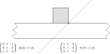
Figure 3. Cut through $B_{\Join}+(-1,1,0)$ at a plane $y=\delta$ (for $\delta>0$ small) and the transformation $\phi_{\blacktriangle}$

The following is straighforward to verify:

• Both transformations coincide on the plane $\{\mathrm{x}\,:\,z=x\}$ and thus together define a globally bi-Lipschitz mapping $\phi_{\blacktriangle}:{\mathbb{R}}^{3}\to{\mathbb{R}}^{3}$, which, additionally, is volume-preserving.

• The intersection of $\phi_{\blacktriangle}\bigl{(}B_{\Join}+(-1,1,0)\bigr{)}$ with a sufficiently small, paraxial cube $\varepsilon K$ around $\mathrm{0}$ equals the set

  $$\{\mathrm{x}\,:\,-\varepsilon<x<0,\ -\varepsilon<y<\varepsilon,\ -\varepsilon<z<0\}\cup\{\mathrm{x}\,:\,0\leq x<\varepsilon,\ 0<y<\varepsilon,\ -\varepsilon<z<0\}.$$

(To prove the latter, note that the $y$-component is left invariant under $\phi_{\blacktriangle}$ and that $\phi_{\blacktriangle}$ acts in the plane $y=0$ as follows: the vector $(0,1)$ is mapped onto $(-1,0)$ and the vector $(-1,0)$ onto $(0,-1)$. Finally, the vector $(1,0)$ is left invariant.) Next we introduce the mapping $\phi_{\triangle}$ which is defined as the linear mapping $\left(\begin{array}[]{rrr}2&1&0\\ -1&0&0\\ 0&0&1\end{array}\right)$ on the set $\{\mathrm{x}\,:\,-x<y\}$ and as the identity on the set $\{\mathrm{x}\,:\,-x\geq y\}$, see Figure 4.

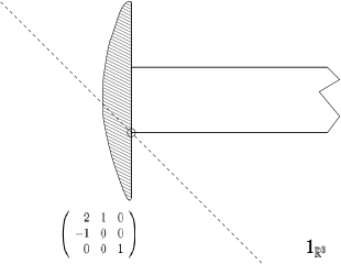
Figure 4. Cut through $\phi_{\blacktriangle}\bigl{(}B_{\Join}+(-1,1,0)\bigr{)}$ at a plane $z=-\delta$ in a neighborhood of $\mathrm{0}$ ($\delta>0$ sufficiently small)

One directly verifies that $\left(\begin{array}[]{rrr}2&1&0\\ -1&0&0\\ 0&0&1\end{array}\right)$ acts as the identity on the set $\{\mathrm{x}\,:\,-x=y\}$; thus $\phi_{\triangle}$ in fact is a bi-Lipschitz, volume-preserving mapping from ${\mathbb{R}}^{3}$ onto itself. After this transformation the resulting object, intersected with a sufficiently small paraxial cube $\varepsilon K$, equals the convex set

$$\{\mathrm{x}\,:\,-\varepsilon<x<\varepsilon,0<y<\varepsilon,-\varepsilon<z<0\}.$$

Here again Remark 3.3 applies, what finishes the proof. ∎

8. Concluding Remarks

Remark 8.1.

The reader may have asked himself why we restricted the considerations to real, symmetric coefficient functions $\mu$. The answer is twofold: first, we need at all costs Gaussian estimates for our techniques and it is known that these are not available for complex coefficients in general, see [11] and also [26]. Additionally, Proposition 4.8 also rests on this supposition. On the other hand, in the applications we have primarly in mind this condition is satisfied.

Remark 8.2.

Under the additional Assumption 6.3, Theorem 5.4 implies maximal parabolic regularity for $-\nabla\cdot\mu\nabla$ on $H^{-1,q}_{\Gamma}$ for every $q\in[2,\infty[$, as in the 2-$d$ case.

Besides, the question arises whether the limitation for the exponents, caused by the localization procedure, is principal in nature or may be overcome when applying alternative ideas and techniques (cf. Theorem 4.4). We do not know the answer at present.

Remark 8.3.

We considered here only the case of one single parabolic equation, but everything can be carried over in a straightforward way to the case of diagonal systems; ’diagonal’ in this case means that the function $\mathcal{G}$ is allowed to depend on the vector $u=(u_{1},\dots,u_{n})$ of solutions and the right hand side also. In the same spirit one can treat triagonal systems.

Remark 8.4.

Inspecting Proposition 6.1, one easily observes that in fact an additional $t$-dependence of the function $\mathcal{G}$ would be admissible. We did not carry this out here for the sake of technical simplicity.

Remark 8.5.

In (1.2) we restricted our setting to the case where the Dirichlet boundary condition is homogeneous. It is straightforward to generalize this to the case of inhomogeneous Dirichlet conditions by splitting off the inhomogeneity, see [40, Ch. II.2] or [23, Ch. 1.2], see also [59] where this has been carried out in detail in the case of parabolic systems.

Remark 8.6.

If one knows a priori that the right hand side of (1.1) depends Hölder continuously on the time variable $t$, then one can use other local existence and uniqueness results for abstract parabolic equations, see e.g. [69] for details. In this case the solution $u$ is even strongly differentiable in the space $X$ (with continuous derivative), what may lead to a better justification of time discretization then, compare [9] and references therein.

Remark 8.7.

Let us explicitely mention that Assumption 6.3 is not always fulfilled in the 3-$d$ case. First, there is the classical counterexample of Meyers, see [74], a simpler (and somewhat more striking) one is constructed in [34], see also [35]. The point, however, is that not the mixed boundary conditions are the obstruction but a somewhat ’irregular’ behavior of the coefficient function $\mu$ in the inner of the domain. If one is confronted with this, spaces with weight may be the way out.

Remark 8.8.

In two and three space dimensions one can give the following simplifying characterization for a set $\Omega\cup\Gamma$ to be regular in the sense of Gröger, i.e. to satisfy Assumption 3.2 a), see [57]:

If $\Omega\subseteq{\mathbb{R}}^{2}$ is a bounded Lipschitz domain and $\Gamma\subseteq\partial\Omega$ is relatively open, then $\Omega\cup\Gamma$ is regular in the sense of Gröger iff $\partial\Omega\setminus\Gamma$ is the finite union of (non-degenerate) closed arc pieces.

In ${\mathbb{R}}^{3}$ the following characterization can be proved, heavily resting on a deep result of Tukia [87]:

If $\Omega\subset{\mathbb{R}}^{3}$ is a Lipschitz domain and $\Gamma\subset\partial\Omega$ is relatively open, then $\Omega\cup\Gamma$ is regular in the sense of Gröger iff the following two conditions are satisfied:

1. $\partial\Omega\setminus\Gamma$ is the closure of its interior (within $\partial\Omega$).

2. for any ${\mathrm{x}}\in\overline{\Gamma}\cap(\partial\Omega\setminus\Gamma)$ there is an open neighborhood $\mathcal{U}\ni{\mathrm{x}}$ and a bi-Lipschitz mapping $\kappa:\mathcal{U}\cap\overline{\Gamma}\cap(\partial\Omega\setminus\Gamma)\to\left]-1,1\right[$.

References

- [1] L. Adams, Z. Li, The immersed interface/multigrid methods for interface problems, SIAM J. Sci. Comput. 24 (2002) 463–479.
- [2] H. Amann, Parabolic evolution equations and nonlinear boundary conditions, J. Differential Equations 72 (1988), no. 2, 201–269.
- [3] H. Amann, Nonhomogeneous linear and quasilinear elliptic and parabolic boundary value problems, in: H.-J. Schmeisser et al. (eds.), Function spaces, differential operators and nonlinear analysis, Teubner-Texte Math., vol. 133, Teubner, Stuttgart, 1993, pp. 9–126.
- [4] H. Amann, Linear and quasilinear parabolic problems, Birkhäuser, Basel-Boston-Berlin, 1995.
- [5] S.N. Antontsev, M. Chipot, The thermistor problem: Existence, smoothness, uniqueness, blowup, SIAM J. Math. Anal. 25 (1994) 1128–1156.
- [6] W. Arendt, Semigroup properties by Gaussian estimates, RIMS Kokyuroku 1009 (1997) 162–180.
- [7] W. Arendt, A.F.M. terElst, Gaussian estimates for second order elliptic operators with boundary conditions, J. Operator Theory 38 (1997) 87–130.
- [8] W. Arendt, Semigroups and evolution equations: functional calculus, regularity and kernel estimates, in: C.M. Dafermos et al. (eds.), Evolutionary equations, Vol. I of Handbook of Differential Equations, Elsevier/North-Holland, Amsterdam, 2004, pp. 1–85.
- [9] A. Ashyralyev, P.E. Sobolevskii, New difference schemes for partial differential equations, Operator Theory: Advances and Applications, vol. 148, Birkhäuser, Basel, 2004.
- [10] P. Auscher, On necessary and sufficient conditions for -estimates of Riesz Transforms Associated to Elliptic Operators on and related estimates, Mem. Amer. Math. Soc. 186 (2007), no. 871.
- [11] P. Auscher, X.T. Duong, P. Tchamitchian, Absence de principe du maximum pour certaines équations paraboliques complexes, Colloq. Math. 71 (1996), no. 1, 87–95.
- [12] P. Auscher, P. Tchamitchian, Square roots of elliptic second order divergence operators on strongly Lipschitz domains: theory, Math. Ann. 320 (2001), no. 3, 577–623.
- [13] A. Axelsson, S. Keith, A. McIntosh, The Kato square root problem for mixed boundary value problems, J. Lond. Math. Soc. (2) 74 (2006), no. 1, 113–130.
- [14] U. Bandelow, R. Hünlich, T. Koprucki, Simulation of static and dynamic properties of edge-emitting multiple-quantum-well lasers, IEEE JSTQE 9 (2003) 798–806.
- [15] C. Bennett, R. Sharpley, Interpolation of operators, Pure and Applied Mathematics, vol. 129, Academic Press, Boston etc., 1988.
- [16] H. Berestycki, F. Hamel, L. Roques, Analysis of the periodically fragmented environment model: I–species persistence, J. Math. Biol. 51 (2005), no. 1, 75–113.
- [17] Y.M. Berezanskij, Selfadjoint operators in spaces of functions of infinitely many variables, Translations of Mathematical Monographs, vol. 63, American Mathematical Society, Providence, R.I., 1986.
- [18] S.-S. Byun, Optimal regularity theory for parabolic equations in divergence form, J. Evol. Equ. 7 (2007), no. 3, 415–428.
- [19] G. Caginalp, X. Chen, Convergence of the phase field model to its sharp interface limits, Eur. J. Appl. Math. 9 (1998), no. 4, 417–445.
- [20] H. Carslaw, J. Jaeger, Conduction of heat in solids, Clarendon Press, New York, 1988.
- [21] N.H. Chang, M. Chipot, On some mixed boundary value problems with nonlocal diffusion, Adv. Math. Sci. Appl. 14 (2004), no. 1, 1–24.
- [22] M. Chipot, B. Lovat, On the asymptotic behavior of some nonlocal problems, Positivity 3 (1999) 65–81.
- [23] P.G. Ciarlet, The finite element method for elliptic problems, Studies in Mathematics and its Applications, vol. 4, North Holland, Amsterdam-New York-Oxford, 1978.
- [24] P. Clement, S. Li, Abstract parabolic quasilinear equations and application to a groundwater flow problem, Adv. Math. Sci. Appl. 3 (1994) 17–32.
- [25] M. Dauge, Neumann and mixed problems on curvilinear polyhedra, Integral Equations Oper. Theory 15 (1992), no. 2, 227–261.
- [26] E.B. Davies, Limits on regularity of self-adjoint elliptic operators, J. Differential Equations 135 (1997), no. 1, 83–102.
- [27] R. Denk, M. Hieber, J. Prüss, -boundedness, Fourier multipliers and problems of elliptic and parabolic type, Mem. Amer. Math. Soc. 166 (2003), no. 788.
- [28] L. de Simon, Un’applicazione della teoria degli integrali singolari allo studio delle equazione differenziali lineari astratte del primo ordine, Rend. Sem. Math. Univ. Padova 34 (1964) 205–223.
- [29] J. Dieudonné, Grundzüge der modernen Analysis 1, VEB Deutscher Verlag der Wissenschaften, Berlin, 1971.
- [30] G. Dore, A. Venni, On the closedness of the sum of two closed operators, Math. Z. 196 (1987) 189–201.
- [31] G. Dore, regularity for abstract differential equations, in: H. Komatsu (ed.), Functional analysis and related topics, Proceedings of the international conference in memory of Professor Kosaku Yosida held at RIMS, Kyoto University, Japan, July 29-Aug. 2, 1991, Lect. Notes Math., vol. 1540, Springer-Verlag, Berlin, 1993, pp. 25–38.
- [32] X.T. Duong, A. Intosh, The boundedness of Riesz transforms associated with divergence form operators, in: Workshop on Analysis and Applications, Brisbane, Proc. Center Math. Anal. 37 (1999), 15–25.
- [33] X.T. Duong, D. Robinson, Semigroup kernels, Poisson bounds, and holomorphic functional calculus, J. Funct. Anal. 142 (1996), no. 1, 89–128.
- [34] J. Elschner, H.-C. Kaiser, J. Rehberg, G. Schmidt, regularity results for elliptic transmission problems on heterogeneous polyhedra, Math. Models Methods Appl. Sci. 17 (2007), no. 4, 593–615.
- [35] J. Elschner, J. Rehberg, G. Schmidt, Optimal regularity for elliptic transmission problems including interfaces, Interfaces Free Bound. 9 (2007) 233–252.
- [36] L.C. Evans, R.F. Gariepy, Measure theory and fine properties of functions, Studies in advanced mathematics, CRC Press, Boca Raton-New York-London-Tokyo, 1992.
- [37] I. Fonseca, G. Parry, Equilibrium configurations of defective crystals, Arch. Rat. Mech. Anal. 120 (1992) 245–283.
- [38] P.C. Franzone, L. Guerri, S. Rovida, Wavefront propagation in an activation model of the anisotropic cardiac tissue: asymptotic analysis and numerical simulation, J. Math. Biol. 28 (1990) 121–176.
- [39] H. Gajewski, K. Gröger, Reaction-diffusion processes of electrical charged species, Math. Nachr. 177 (1996) 109–130.
- [40] H. Gajewski, K. Gröger, K. Zacharias, Nichtlineare Operatorgleichungen und Operatordifferentialgleichungen, Akademie-Verlag, Berlin, 1974.
- [41] H. Gajewski, I.V. Skrypnik, On the uniqueness of solutions for nonlinear elliptic-parabolic problems, J. Evol. Equ. 3 (2003) 247–281.
- [42] G. Giacomin, J.L. Lebowitz, Phase segregation in particle systems with long-range interactions. I. Macroscopic limits, J. Statist. Phys. 87 (1997) 37–61.
- [43] by same author, Phase segregation in particle systems with long-range interactions. II. Interface motion, SIAM J. Appl. Math. 58 (1998) 1707–1729.
- [44] M. Giaquinta, M. Struwe, An optimal regularity result for a class of quasilinear parabolic systems, Manuscr. Math. 36 (1981) 223–239.
- [45] E. Giusti, Metodi diretti nel calcolo delle variazioni, Unione Matematica Italiana, Bologna, 1994.
- [46] J.A. Griepentrog, On the unique solvability of a nonlocal phase separation problem for multicomponent systems, Banach Center Publications 66 (2004) 153–164.
- [47] J.A. Griepentrog, W. Höppner, H.-C. Kaiser, J. Rehberg, A bi-Lipschitz, volume-preserving map form the unit ball onto the cube, WIAS-Preprint 1048, Berlin, 2005, to appear in Note di Matematica.
- [48] J.A. Griepentrog, K. Gröger, H. C. Kaiser, J. Rehberg, Interpolation for function spaces related to mixed boundary value problems, Math. Nachr. 241 (2002) 110–120.
- [49] J.A. Griepentrog, H.-C. Kaiser, J. Rehberg, Heat kernel and resolvent properties for second order elliptic differential operators with general boundary conditions on , Adv. Math. Sci. Appl. 11 (2001) 87–112.
- [50] J.A. Griepentrog, Linear elliptic boundary value problems with non-smooth data: Campanato spaces of functionals, Math. Nachr. 243 (2002) 19–42.
- [51] J.A. Griepentrog, Maximal regularity for nonsmooth parabolic problems in Sobolev-Morrey spaces, Adv. Differential Equations 12 (2007), no. 9, 1031–1078.
- [52] P. Grisvard, Elliptic problems in nonsmooth domains, Pitman, Boston, 1985.
- [53] K. Gröger, A -estimate for solutions to mixed boundary value problems for second order elliptic differential equations, Math. Ann. 283 (1989) 679–687.
- [54] K. Gröger, J. Rehberg, Resolvent estimates in for second order elliptic differential operators in case of mixed boundary conditions, Math. Ann. 285 (1989), no. 1, 105–113.
- [55] K. Gröger, -estimates of solutions to evolution equations corresponding to nonsmooth second order elliptic differential operators, Nonlinear Anal. 18 (1992), no. 6, 569–577.
- [56] R. Haller-Dintelmann, H.-C. Kaiser, J. Rehberg, Elliptic model problems including mixed boundary conditions and material heterogeneities, J. Math. Pures Appl. 89 (2008) 25–48.
- [57] R. Haller-Dintelmann, C. Meyer, J. Rehberg, Hölder continuity for second order elliptic problems with nonsmooth data, in preparation.
- [58] M. Heinkenschloss, F. Troeltzsch, Analysis of the Langrange-SQP-Newton method for the control of a phase field equation, Control and Cybernetics 28 (1999), no. 2, 177–211.
- [59] M. Hieber, J. Rehberg, Quasilinear parabolic systems with mixed boundary conditions, WIAS-Preprint no. 1124, Berlin, 2006, to appear in SIAM J. Math. Anal.
- [60] D. Jerison, C. Kenig, The inhomogeneous Dirichlet problem in Lipschitz domains, J. Funct. Anal. 130 (1995), no. 1, 161–219.
- [61] A. Jonsson, H. Wallin, Function spaces on subsets of , Math. Rep. 2 (1984), no. 1.
- [62] N. Kalton, P. Kunstmann, L. Weis, Perturbation and interpolation theorems for the -calculus with applications to differential operators, Math. Ann. 336 (2006) 747–801.
- [63] E. Kapon, Semiconductor Lasers I, Academic Press, Boston, 1999.
- [64] T. Kato, Perturbation theory for linear operators, Reprint of the corr. print. of the 2nd ed., Classics in Mathematics, Springer-Verlag, Berlin, 1980.
- [65] P. Krejci, E. Rocca, J. Sprekels, Nonlocal temperature-dependent phase-field models for non-isothermal phase transitions, WIAS-Preprint no. 1006, Berlin, 2005.
- [66] P.C. Kunstmann, Heat kernel estimates and spectral independence of elliptic operators, Bull. London Math. Soc. 31 (1999) 345–353.
- [67] P.C. Kunstmann, L. Weis, Perturbation theorems for maximal -regularity, Ann. Sc. Norm. Super. Pisa Cl. Sci. (4) 30 (2001), no. 2, 415–435.
- [68] O.A. Ladyzhenskaya, V.A. Solonnikov, N.N. Ural’tseva, Linear and quasi-linear equations of parabolic type, Translations of Mathematical Monographs, vol. 23., American Mathematical Society (AMS), Providence, RI, 1967.
- [69] A. Lunardi, Abstract quasilinear parabolic equations, Math. Ann. 267 (1984) 395–415.
- [70] V.G. Maz’ya, Sobolev spaces, Springer, Berlin-Heidelberg-New York-Tokyo, 1985.
- [71] V. Maz’ya, J. Elschner, J. Rehberg, G. Schmidt, Solutions for quasilinear nonsmooth evolution systems in , Arch. Rational Mech. Anal. 171 (2004), no. 2, 219–262.
- [72] V. Maz’ya, T.O. Shaposhnikova, Theory of multipliers in spaces of differentiable functions, Monographs and Studies in Mathematics, vol. 23, Pitman, Boston-London-Melbourne, 1985.
- [73] A. Intosh, Operators which have an functional calculus, in: Miniconference on operator theory and partial differential equations (North Ryde, 1986), Proc. Centre Math. Anal. Austral. Nat. Univ., vol. 14, Austral. Nat. Univ., Canberra, 1986, pp. 210–231.
- [74] N. Meyers, An -estimate for the gradient of solutions of second order elliptic divergence equations, Ann. Sc. Norm. Super. Pisa, Sci. Fis. Mat. (3) 17 (1963) 189–206.
- [75] E. Ouhabaz, Analysis of Heat Equations on Domains, London Mathematical Society Monographs Series, vol. 31, Princeton University Press, Princeton, 2005.
- [76] A. Pazy, Semigroups of linear operators and applications to partial differential equations, Springer, 1983.
- [77] J. Prüss, Maximal regularity for evolution equations in -spaces, Conf. Semin. Mat. Univ. Bari 285 (2002) 1–39.
- [78] J. Quastel, Diffusion of color in the simple exclusion process, Comm. Pure Appl. Math. 45 (1992), no. 6, 623–679.
- [79] J. Quastel, F. Rezakhanlou, S.R.S. Varadhan, Large deviations for the symmetric exclusion process in dimension , Probab. Theory Relat. Fields 113 (1999) 1–84.
- [80] S. Selberherr, Analysis and simulation of semiconductor devices, Springer, Wien, 1984.
- [81] E. Shamir, Regularization of mixed second-order elliptic problems, Isr. J. Math. 6 (1968) 150–168.
- [82] I. Sneiberg, Spectral properties of linear operators in families of Banach spaces, Mat. Issled. 9 (1974) 214–229.
- [83] A. Sommerfeld, Thermodynamics and statistical mechanics (Lectures on theoretical physics, vol. V.), Academic Press, New York, 1956.
- [84] M. Struwe, On the Hölder continuity of bounded weak solutions of quasilinear parabolic systems, Manuscr. Math. 35 (1981) 125–145.
- [85] H. Triebel, Interpolation theory, function spaces, differential operators, North Holland Publishing Company, Amsterdam-New York-Oxford, 1978.
- [86] H. Triebel, On spaces of and type, Math. Nachr. 85, (1978) 75–90.
- [87] P. Tukia, The planar Schönflies theorem for Lipschitz maps, Ann. Acad. Sci. Fenn. Ser. A I Vol. 5 (1980), no. 1, 49–72.
- [88] A. Unger, F. Troeltzsch, Fast solutions of optimal control problems in the selective cooling of steel, ZAMM 81 (2001), no. 7, 447–456.
- [89] J. Wloka, Partial differential equations, Cambridge University Press, Cambridge, 1987.
- [90] W.P. Ziemer, Weakly differentiable functions. Sobolev spaces and functions of bounded variation, Graduate Texts in Mathematics, vol. 120, Springer-Verlag, Berlin etc., 1989.