Geometric interpretation of pre-vitrification in hard sphere liquids

Abstract

We derive a microscopic criterion for the stability of hard sphere configurations, and we show empirically that this criterion is marginally satisfied in the glass. This observation supports a geometric interpretation for the initial rapid rise of viscosity with packing fraction, or pre-vitrification. It also implies that barely stable soft modes characterize the glass structure, whose spatial extension is estimated. We show that both the short-term dynamics and activation processes occur mostly along those soft modes, and we study some implications of these observations. This article synthesizes new and previous results [C. Brito and M. Wyart, Euro. Phys. Letters, 76, 149-155, (2006) and C. Brito and M. Wyart, J. Stat. Mech., L08003 (2007) ] in a unified view.

I Introduction

Unlike crystals, amorphous structures are poorly understood on small length scales. This is apparent when one considers the low-temperature properties of glasses such as heat transport andy and the nature of the two-level systems leading to a linear specific heat philips , or the statistics of force chains and stress propagation in a pile of sand force . Part of the difficulty comes from the out-of-equilibrium nature of amorphous solids: to understand their structure and properties, one must also understand how they are made. This is the difficult problem of the glass or jamming transition, where a fluid stops flowing and rest in some meta-stable configuration. At the center of this phenomenon lies a geometrical question: by which processes can a dense assembly of particles rearrange, and how do these rearrangements depend on the particles packing?

It is surprising that a similar question has been solved in the 70’s on the apparently more complicated problem of polymers entanglement reptation , where the objects considered are not simple particles but long chains forming a melt. In our view part of the reason for this paradox is the following: in a melt, the relaxation time scales with the length of the polymers. This fact can be captured experimentally and is a stringent test for theories. The situation is very different in glasses, where the length scales at play appear to be limited heterog . This fact makes it harder to distinguish and compare the predictions of different theories. Nevertheless, recent numerics suggests that the length scales at play may not always be small. Particles interacting with a purely repulsive short-range potential display a critical point, corresponding to jammed packings for which the overlaps between particles vanish. Near that point, scaling laws characterize the microscopic structure J ; these_matt ; torquato , elastic J ; these_matt ; sil ; matthieu3 ; saarloos and transport ning properties, and relaxation in shear flows olsson .

A particularly interesting observation is that soft modes, collective displacement of particles with a small restoring force, are abundant near this critical point J . The relation between the microscopic structure and the characteristic frequency and length scale of these modes was derived, and in particular the latter was shown to diverge near threshold matthieu1 . In turn, imposing the stability of these modes led to the derivation of a non-trivial microscopic criterion for packing of repulsive particles matthieu2 , that any mechanically stable configuration must satisfy. For infinitely fast quench followed by adiabatic decompression, it was observed that this criterion is marginally satisfied J ; matthieu2 : configurations generated by such a protocol are barely stable. This supported that at least for an infinitely fast quench, the realization of this microscopic criterion affects the dynamics, and suggested that soft modes may play a role in the structural rearrangements of particles. To show that this is the case in the empirically relevant situation of a slow quench, one would have to study a super-cooled liquid at finite temperature, and analyze soft modes, microscopic structure and relaxation together. This is what we perform here, using hard spheres, where interactions are purely entropic and where a critical point also turns out to be present, allowing a scaling analysis.

The paper is organized as follows. We start by illustrating the key results on the soft modes and the stability of packing of elastic particles using a simple model, the square lattice. In Section III, after defining the coordination of a hard sphere configuration, we establish a mapping between the free energy of a hard sphere system and the energy of an elastic network. This enables to apply all the conceptual tools developed in elastic systems to hard particles, in particular we derive a microscopic criterion for the stability of hard sphere configurations. In Section IV we present the numerical protocol we use, both in the glass and the super-cooled liquid, to identify meta-stable states and characterize their structural properties. In Section V we show that in those meta-stable states the stability criterion is saturated: configurations visited are barely stable mechanically. We confirm this observation in Section VI where the short term dynamics is studied. The marginal stability of the glass implies in particular an anomalous scaling for the mean square displacement near maximum packing, which we check numerically. In Section VII it is shown that only a small fraction of the degrees of freedom of the system participate to activation events where new meta-stable states are visited. Those degrees of freedom are precisely the soft modes present in the glass structure. Finally we argue that these observations support a geometric interpretation for pre-vitrification, which is presented in Section VIII.

II A criterion for the mechanical stability of elastic networks

Studying engineering structures, Maxwell max established a necessary criterion for the mechanical stability of elastic networks. The key microscopic parameter is the coordination $z$, the average number of interactions per particle. For an elastic network of springs, his criterion reads $z>z_{c}=2d$, where $d$ is the spatial dimension of the system. The demonstration goes as follows. Consider a set of $N$ points interacting with $N_{c}$ springs, at rest, of stiffness $k$. The expansion of the energy is:

$$\delta E=\sum_{\langle ij\rangle}\frac{k}{2}[(\delta{\vec{R}_{i}}-\delta{\vec{R}_{j}})\cdot{\vec{n}_{ij}}]^{2}+o(\delta R^{2}),$$ (1)

where the sum is made over all springs, ${\vec{n}_{ij}}$ is the unit vector going from $i$ to $j$, and $\delta{\vec{R}_{i}}$ is the displacement of particles $i$. A system is floppy, i.e. not mechanically stable, if it can be deformed without energy cost, that is if there is a displacement field for which $\delta E=0$, or equivalently $(\delta{\vec{R}_{i}}-\delta{\vec{R}_{j}})\cdot{\vec{n}_{ij}}=0$ $\forall ij$. If the spatial dimension is $d$, this linear system has $Nd$ degrees of freedom (ignoring the $d(d+1)/2$ rigid motions of the entire system) and $N_{c}\equiv Nz/2$ equations, and therefore there are always non-trivial solutions if $Nd>N_{c}$, that is if $z<2d\equiv z_{c}$. Finite stiffness therefore requires:

$$z\geq 2d.$$ (2)

Under compression, the criterion of rigidity becomes more demanding. Here we illustrate this result in a simple model, but the different scaling we obtain have broader applications and are valid in particular for random assemblies of elastic particles matthieu1 ; matthieu2 . Consider a square lattice of springs of rest length $\sigma$. It marginally satisfies the Maxwell criterion, since $z=4$ and $d=2$. We add randomly a density $\delta z$ of springs at rest connecting second neighbors, represented as dotted lines in Fig(1), such that the coordination is $z=z_{c}+\delta z$. Springs are added in a rather homogeneous manner, so that there are not large regions without dotted springs. The typical distance between two dotted springs in a given row or column is then:

$$l^{*}\sim\sigma/\delta z$$ (3)

How much pressure $p$ can this system sustain before collapsing? To be mechanically stable, all collective displacements must have a positive energetic cost. It turns out that the first modes to collapse as the pressure is increased are of the type of the longitudinal modes of wavelength $l^{*}$ of individual segments of springs contained between two dotted diagonal springs as represented with arrows in Fig(1). These modes have a displacement field of the form $\delta{\vec{R}_{i}}=2X\sin(\pi i\sigma/l^{*})/\sqrt{l^{*}/\sigma}{\vec{e}_{x}}$, where $i$ labels the particles along a segment and runs between 0 and $l^{*}/\sigma$, ${\vec{e}_{x}}$ is the unit vector in the direction of the line, and $X$ is the amplitude of the mode, $X=1$ for a normalized mode. In the absence of pressure $p$, springs carry no force. The energy of such a mode comes only from the springs of the segment and from Eq.(1) follows $\delta E\sim kX^{2}\sigma^{2}/l^{*}{}^{2}$. Note that these modes have a characteristic frequency:

$$\omega^{*}\sim\sqrt{\frac{\delta E(X=1)}{m}}\sim\sqrt{\frac{k}{m}}\delta z$$ (4)

When $p>0$, each spring now carries a force of order $f\sim p\sigma^{d-1}$. The energy expansion then contains other terms not indicated in Eq.(1) shlomon ; matthieu2 , whose effect can be estimated quantitatively as follows. When particles are displaced along a longitudinal mode such as the one represented by arrows in Fig.(1), the force of each spring directly connected and transverse to the segment considered, represented in dashed line in Fig(1), now produces a work equal to $f$ times the elongation of the spring. This elongation is simply $\delta{\vec{R}_{i}}^{2}/\sigma$ following Pythagoras’ theorem. Summing on all the springs transverse to the segment leads to a work of order $fX^{2}/\sigma$. This gives finally for the energy of the mode $\delta E\sim kX^{2}\sigma^{2}/l^{*}{}^{2}-fX^{2}/\sigma$, where numerical pre-factors are omitted. Stability requires $\delta E>0$, implying that $k\sigma^{3}/l^{*}{}^{2}>f$, or:

$$\delta z>A(f/k\sigma)^{1/2}\sim\sqrt{e}$$ (5)

where A is a numerical constant and $e$ is the typical strain in the contacts. This result signifies that pressure has a destabilizing effect, which needs to be counterbalanced by the creation of more contacts to maintain elastic stability. Note that Eqs.(3,4,5) are more general that the simple square lattice model considered here, they apply to elastic network or assemblies of elastic particles matthieu1 ; matthieu2 as long as spatial fluctuations in coordination are limited.

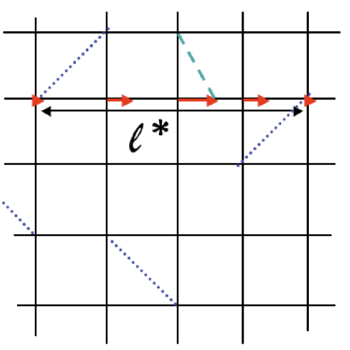
Figure 1: Square lattice of springs with a density per particle $\delta z$ of additional diagonal springs, represented in dotted lines. $l^{*}\sim\sigma/\delta z$ is the typical dimensionless distance of the segments contained between two diagonal springs on a given row or column. The arrows represent the longitudinal mode of wavelength $\sim l^{*}$ of such a segment: $\delta{\vec{R}_{i}}\sim\sin(\pi i\sigma/l^{*}){\vec{e}_{x}}$, following the notation introduced in the text. The dashed line exemplifies the deformation of a spring transverse and directly connected to the segment considered, it is elongated by the longitudinal vibration of this segment. When the pressure is positive and contacts are under compression, this elongation lowers the energy contained in those springs. This leads to an elastic instability when $\delta z$ becomes smaller than a quantity proportional to the square root of the contact strain, of order $f/k\sigma$.

III An analogy between hard sphere glasses and elastic networks

These results on the stability of elastic networks apply to hard spheres systems. In order to see that, we recall the analogy between the free energy of a hard sphere glass and the energy of an athermal network of logarithm springs brito . Consider the dynamics (brownian or newtonian) of hard spheres in a super-cooled liquid or glass state, such that the collision time among neighbor particles $\tau_{c}$ is much smaller than $\tau$, the time scale on which the structure rearranges. On intermediate time scale $t_{1}$ such that $\tau_{c}<<t_{1}<<\tau$ one can define a contact network, by considering all the pairs of particles colliding with each other, those are said to be “in contact” (examples of contact network are shown in the next section). This enables to define a coordination number $z$. Once the contact network is defined in a meta-stable state, all configurations for which particles in contact do not interpenetrate are equiprobable, those configurations satisfy $\prod_{\langle ij\rangle}\Theta(||{\vec{R}_{i}}-{\vec{R}_{j}}||-\sigma)=1$, where $\Theta$ is the Heaviside function, the product is made on all contacts $ij$ and $\sigma$ is the particles diameter, that defines our unit length. The isobaric partition function is then:

$${\cal Z}=\int dV\prod_{i}\int d{\vec{R}_{i}}\prod_{\langle ij\rangle}\Theta(||{\vec{R}_{i}}-{\vec{R}_{j}}||-\sigma)exp(\frac{-pV}{k_{b}T})$$ (6)

In one spatial dimension (for a neckless of spheres), Eq.(6) can be readily solved by changing variables and considering the gaps $h_{ij}=R_{j}-R_{i}$ between particles in contact. The mapping is one to one and linear:

$$\prod_{i}dR_{i}\propto\prod_{ij}dh_{ij}\delta(\sum_{ij}h_{ij}-(V-V_{0}))$$ (7)

where $V_{0}$ is the volume of the system at $p=\infty$. Eqs.(6,7) lead to:

$${\cal Z}=\prod_{ij}\int_{h_{ij}\geq 0}dh_{ij}exp(\frac{-ph_{ij}}{k_{b}T})$$ (8)

leading to the simple result $p=k_{b}T/\langle h\rangle$. In higher dimensions, the situation is far more complicated in general, because the mapping between positions and gaps in not one-to-one, and not linear. There is nevertheless an exception to that rule. As was shown by several authors tom1 ; moukarzel ; roux , as the pressure diverges near maximum packing the system becomes isostatic $z\rightarrow z_{c}$, see footnote for a sketch of the argument. As noted in brito , this implies precisely that the number of contact is equal to the number of degrees of freedom, and that the mapping of particle positions toward the gaps is one-to-one. Near maximum pressure this mapping is also linear as $(d{\vec{R}_{i}}-d{\vec{R}_{j}})\cdot{\vec{n}_{ij}}=dh_{ij}+O(\delta{\vec{R}}^{2})$. One gets:

$$\prod_{i}d{\vec{R}_{i}}\propto\prod_{ij}dh_{ij}\delta(\sum_{ij}f_{ij}h_{ij}-p(V-V_{0}))$$ (9)

where $f_{ij}$ is the force in the contact $ij$. The volume constraint $\delta(\sum_{ij}f_{ij}h_{ij}-p(V-V_{0}))$ generalizes for $d>1$ the constraint $\delta(\sum_{ij}h_{ij}-(V-V_{0}))$. This relation between gaps and volume can be derived as follows. In a meta-stable state, forces must be balance on all particles. As a consequence, the virtual force theorem implies that the work of any displacement is zero: $dW=\sum_{ij}f_{ij}dh_{ij}-pdV=0$. Integrating this relation leads to the relation above . Eqs(6,9) lead to:

$${\cal Z}=\prod_{\langle ij\rangle}\int_{h_{ij}\geq 0}dh_{ij}e^{-f_{ij}h_{ij}/k_{b}T}.$$ (10)

and:

$$f_{ij}=\frac{k_{b}T}{\langle h_{ij}\rangle}$$ (11)

The force is inversely proportional to the average gap between particles, as we shall confirm numerically in the next section. The stiffness in the contact $ij$ is then:

$$k_{ij}=(k_{b}T)/\langle h_{ij}\rangle^{2}$$ (12)

From Eq.(10) one obtains for the Gibbs free energy ${\cal G}$:

$${\cal G}=-k_{b}T\sum_{\langle ij\rangle}\ln(\langle h_{ij}\rangle)=-k_{b}T\sum_{\langle ij\rangle}\ln(r_{ij}^{eq}-\sigma)$$ (13)

where $r_{ij}^{eq}$ is the average distance between particle $i$ and $j$: $r_{ij}^{eq}=\langle||{\vec{R}_{i}}-{\vec{R}_{j}}||\rangle$. Thus the Gibbs free energy of a hard sphere system is equivalent to the energy of a network of logarithmic springs. As for an elastic network, one can define a dynamical matrix ${\cal M}$ by differentiating Eq.(13). ${\cal M}$ describe the linear response of the average displacement of the particles to any applied force field. The eigenvectors of ${\cal M}$ define the normal modes of the free energy Ashcroft .

When $z\geq z_{c}$, as is the case in the glass phase (see below), Eqs.(10-13) are not exact. Nevertheless, the relative deviations to Eq.(11) can be estimated these_matt , and are of order $\delta z=z-z_{c}$. Numerically these corrections turn out to be small (smaller than 5% throughout the glass phase brito ), and we shall neglect them. We will check this approximation further when we study the microscopic dynamics, see Section VI. Then, together with Eq.(5) and Eq.(12), the present analogy leads to the prediction that minima of the free energy in hard spheres system must satisfy:

$$\delta z\geq A\sqrt{e}\sim\sqrt{\langle h\rangle/\sigma}\sim\sqrt{\frac{k_{B}T}{\sigma\langle f\rangle}}.$$ (14)

where $\langle h\rangle$ and $\langle f\rangle$ are the typical gaps and forces between particles in contact, and where Eq.(11) was used to relate these two quantities.

IV Numerical protocol

To study if the meta-stable states visited in the super-cooled liquid and the glass live close to the bound of Eq.(14), and if the proximity of this bound affect the dynamics, we simulate hard discs with Newtonian dynamics: we use an event-driven code Allen_book , particles are in free flight until they collide elastically. We use two-dimensional bidisperse systems of $N=64,256$ and $N=1024$ particles. Half of the particles have a diameter $\sigma_{1}$, which defines our unit length. Other particles have diameter $\sigma_{2}=1.4\sigma_{1}$. All particles have a mass $m$, our unit mass. Since for hard particles $k_{b}T$ is only re-scaling time and energy, we chose $k_{b}T$ as our unit of energy. Our unit of time is then $\sigma_{1}\sqrt{m/k_{b}T}$. All data below are presented in dimensionless quantities.

We seek to study both the glass and the super-cooled liquid phase. To generate configurations with large packing fractions in the glass we use the jammed configurations of J with packing fraction distributed around $\phi_{c}\approx 0.83$. At $\phi_{c}$ the particles are in permanent contact. By reducing the particles diameters by a relative amount $\epsilon$, we obtain configurations of packing fraction $\phi=\phi_{c}(1-\epsilon)^{2}$. We then assign a random velocity to every particle and launch an event-driven simulation. This procedure enables to study the aging dynamics of highly dense systems. For $\phi<\phi_{0}\approx 0.79$, the system is a super-cooled liquid, and can be equilibrated.

IV.1 Numerical definition of meta-stable states

Computing numerically the contact network requires time-averaging on some scale $t_{1}$ such that $\tau_{c}<<t_{1}<<\tau$, where $\tau$ is the $\alpha$-relaxation time of the system, which we define as the time for which the self scattering function decays by 70%. In the super-cooled liquid a natural way to proceed would be to compute $\tau$, and chose $t_{1}<<\tau$. Nevertheless this procedure is not appropriate for the aging dynamics in the glass phase, where $\tau$ is not well defined, and where the dynamics depends on the waiting time. As an alternative protocol, we consider the self-density correlation function not averaged in time:

$$C(\vec{q},t,t_{w})=\langle e^{i\vec{q}.(\vec{R}_{j}(t+t_{w})-\vec{R}_{j}(t_{w}))}\rangle_{j},$$ (15)

where the average is made on every particle $j$ but not on time, $\vec{R}_{j}(t)$ is the position of particle $j$ at time $t$ and $\vec{q}$ is some wave vector. In what follows $||{\vec{q}}||=2\pi/\sigma_{1}$. For all the system sizes we consider in the glass phase, and for small systems (for $N=64$ and to a lower extent for $N=256$) near the glass transition, we observe that $C(\vec{q},t,t_{w})$ displays long and well-defined plateaus interrupted by sudden jumps, as exemplified in Fig.(2). In the super-cooled liquid, those jumps are of order one, indicating that the life time of the plateaus are of order $\tau$ (a few jumps de-correlate the structure). The existence of plateaus interrupted by sharp transitions indicates that the dynamics is intermittent, as previously observed kob ; heuer . In real space, the plateaus of $C(\vec{q},t,t_{w})$ correspond to quiet periods where particles are rapidly rattling around their average position. The jumps indicate rapid and collective rearrangements of the particles. In what follows we call “meta-stable states” those quiet periods of the dynamics. Average quantities are then computed in a given meta-stable state by choosing a time interval $[t,t+t_{1}]$ for which the system lies in the same meta-stable state. We find that average quantities do not vary significantly with the location and the length of the time interval as long as $t_{1}>>\tau_{c}$. This robustness is proven for vibrational modes in particular in Annex 2. In what follows we chose $t_{1}\sim 200\tau_{c}$.

This protocol has the advantage to be applicable both to aging and equilibrated dynamics. On the other hand, it is limited to rather small systems in the liquid phase. Clearly for an infinite system $C(\vec{q},t,t_{w})$ is spatially self-averaging, and smooth. Already for $N=1024$ near the glass transition plateaus are hardly detectable, and our protocol does not apply (although it does in the glass). For such system sizes, the more traditional method (computing $\tau$ from the decay of the smooth self-scattering function and considering some time scale $t_{1}<<\tau$) should be used.

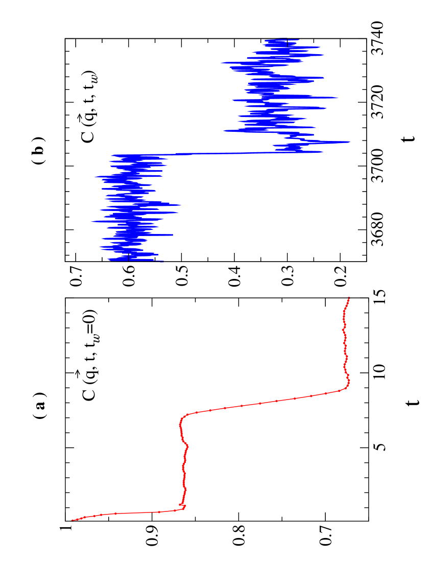
Figure 2: Examples of $C(\vec{q},t,t_{\omega})$ as defined in Eq.(15) vs $t$ (a) in the glass and (b) in the super-cooled liquid.

IV.2 Contact force network

A straightforward quantity to define in a meta-stable state is the average position of the particles:

$$\vec{R}_{i}^{eq}=\frac{1}{t_{1}}\int_{t}^{t+t_{1}}\vec{R}_{i}(t^{\prime})dt^{\prime}.$$ (16)

Central to our analysis is the definition of a contact force network brito ; bubble ; donev2 . Two particles are said to be in contact if they collide with each other during the time interval $t_{1}$. This enables to define an average coordination number $z$ as $z=2N_{c}/N$, where $N_{c}$ is the total number of contacts among all particles of the system. The contact force $\vec{f}_{ij}$ between these particles is then defined as average momentum they exchange per unit of time:

$$\vec{f}_{ij}=\frac{1}{t_{1}}\sum_{n=1}^{n=n_{col}[t_{1}]}\Delta\vec{P}_{n},$$ (17)

where the sum is made on the total number of collisions $n_{col}[t_{1}]$ between $i$ and $j$ that took place in the time interval $t_{1}$, and $\Delta\vec{P}_{n}$ is the momentum exchanged at the $n$th chock. Fig.(3) shows a contact force network obtained using this procedure, and Fig.(4) shows the amplitude of the contact force as a function of the average gap between the particles in contact.

We define the average contact force of the network $\langle f\rangle$ as:

$$\langle f\rangle = \frac{1}{N}\sum_{\langle ij\rangle}^{N}||\vec{f}_{ij}||.$$ (18)

Near maximum packing $\langle f\rangle$ scales as the pressure $p$ and as the inverse of the average gap $h=\langle h_{ij}\rangle$, as implied by Eq.(11). The densest packing fraction $\phi_{0}\approx 0.79$ we can equilibrate corresponds to $\langle f\rangle\approx 18$. For larger values of $\langle f\rangle$, the system is a glass.

Figure 3: Contact forces for $N=256$, $\langle f\rangle=6740$ and $t_{1}=10^{4}$ time steps. Points represent particles centers. Contact forces are sketched by line segments which link particles that are in contact. The width of these segments is proportional to the force amplitude. This figure has already been published in the reference “On the rigidity of hard sphere glass near random close packing”, Europhyscis Letters, v 76, 149-155 (2006) by C. Brito and M. Wyart and it is reproduced here under permission of the Institute of Physics Publishing (IOP).

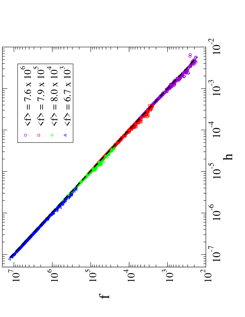
Figure 4: Log-log plot of the amplitude of the contact force vs the gap between the particles for different values of $\langle f\rangle$ in a system with $N=256$ particles. Each point corresponds to a pair of numbers ($f_{ij},\langle h_{ij}\rangle$) that characterizes a pair of particles in contact. The slashed line is a fit of the theoretical relation predicted in Eq.(11). This figure has already been published in the reference “On the rigidity of hard sphere glass near random close packing”, Europhyscis Letters, v 76, 149-155 (2006) by C. Brito and M. Wyart and it is reproduced here under permission of the Institute of Physics Publishing (IOP).

Note that close to maximum packing, at very large pressure, a few percents of the particles do not contribute to the rigidity of the structure. These “rattlers” appears in Fig.(3) as particles which do not exchange forces with any neighbors. In our analysis below we systematically remove such particles, and the procedure we use to do so is presented in Annex 1.

IV.3 Normal modes of the free energy

As shown in Eq.(13), the free energy in a meta-stable state can be written in terms of the average particle positions. It follows that it can be expanded for small average displacements. For discs ($d=2$) this reads:

$$\delta{\cal G}\approx-\sum_{\langle ij\rangle}\frac{1}{\langle h_{ij}\rangle}\frac{[(\delta\vec{R_{j}}-\delta\vec{R_{i}})\cdot{\vec{n}_{ij}}^{\bot}]^{2}}{2r_{ij}^{eq}}+$$ (19)

$$\sum_{\langle ij\rangle}\frac{1}{2\langle h_{ij}\rangle^{2}}[(\delta\vec{R_{j}}-\delta\vec{R_{i}}).\vec{n}_{ij}]^{2}+o(\delta R^{2})$$

where ${\vec{n}_{ij}}^{\bot}$ is the unit vector orthogonal to ${\vec{n}_{ij}}$. Eq.(19) can be written in matrix form:

$$\delta{\cal G}=\langle\delta{\bf R}|{\cal M}|\delta{\bf R}\rangle$$ (20)

where $|\delta{\bf R}\rangle$ is the dN-dimensional vector $\delta\vec{R_{1}}..\delta\vec{R_{N}}$ and $\langle\delta{\bf R}^{\alpha}|\delta{\bf R}^{\beta}\rangle\equiv\sum_{i}^{N}\delta\vec{R_{i}}^{\alpha}\cdot\delta\vec{R_{i}}^{\beta}$. ${\cal M}$ is the dynamical (or stiffness) matrix. For completeness, note that for discs it can be written as a $N\times N$ matrix whose elements ${\cal M}_{ij}$ are tensors of rank $d$, for $d=2$ this reads:

$${\cal M}_{ij}=-\delta_{\langle ij\rangle}(\frac{1}{2r_{ij}^{eq}\langle h_{ij}\rangle}\vec{n}_{ij}^{\bot}\otimes\vec{n}_{ij}^{\bot}-\frac{1}{2\langle h_{ij}\rangle^{2}}~{}\vec{n}_{ij}\otimes\vec{n}_{ij})+$$

$$\delta_{i,j}\sum_{\langle l\rangle}(\frac{1}{2r_{ij}^{eq}\langle h_{il}\rangle}~{}\vec{n}_{ij}^{\bot}\otimes\vec{n}_{ij}^{\bot}-\frac{1}{2\langle h_{il}\rangle^{2}}~{}\vec{n}_{il}\otimes\vec{n}_{il}),$$

where $\delta_{\langle ij\rangle}=1$ when particles $i$ and $j$ are in contact and where the second sum is made on all the particles $\langle l\rangle$ in contacts with the particle $i$. $\otimes$ is the tensor product. ${\cal M}$ describes the linear response of the average displacement of the particles to an external force. The eingenvectors of ${\cal M}$ are the normal modes of the system and the frequencies are the square roots of these eigenvalues clapack . The distribution of these frequencies is the density of states $D(\omega)$. We shall denote $|\delta{\bf R}^{\omega}\rangle$ the displacement field of a normal mode of frequency $\omega$. These modes form a complete orthonormal basis $\{|\delta{\bf R}^{\omega}\rangle\}$.

V Marginal stability of the microscopic structure

According to Eq.(14), minima of the free energy must have a sufficiently coordinated contact network. One may ask if the meta-stable states generated dynamically satisfy this bound easily, or marginallybrito . In order to test this question, we prepare systems at various pressures and identify meta-stable states. Deep in the glass phase, starting from some initial condition typically 3 or 4 states are visited during aging on the time scales we explore. During aging the pressure can drop by several orders of magnitudes (indicating the possibility to obtain denser jammed configurations under re-compression, i.e. larger $\phi_{c}$). For each meta-stable state visited, we measure the coordination of the contact force network, and the average force $\langle f\rangle$. The corresponding data is presented in Fig.(5), together with measures of the coordination in the super-cooled liquid where equilibrium is reached.

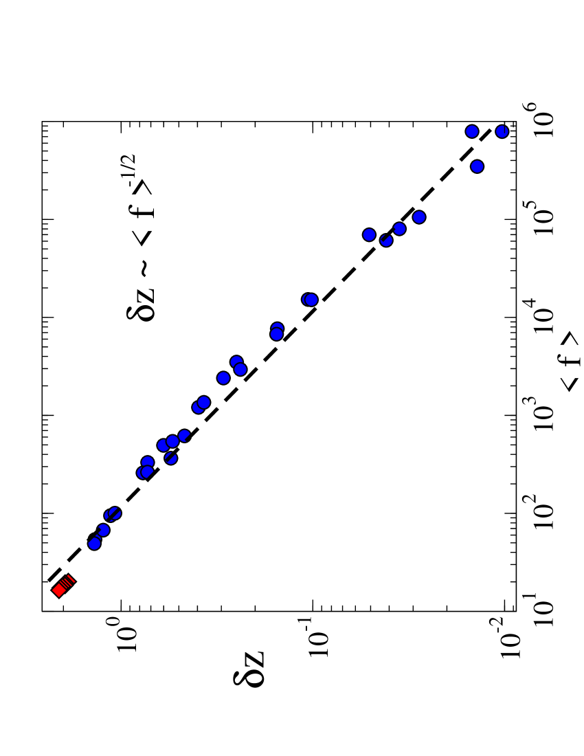
Figure 5: Log-log plot of $\delta z$ vs $\langle f\rangle$ for $N=256$ or $N=1024$ particles. Each circle correspond to one meta-stable state in the glass phase, whereas diamonds correspond to averaged quantity among 11 meta-stable states in the super-cooled liquid. The slashed line is the best fit of the form $\delta z=A\langle f\rangle^{-1/2}$. This figure has already been published in the reference “On the rigidity of hard sphere glass near random close packing”, Europhyscis Letters, v 76, 149-155 (2006) by C. Brito and M. Wyart and it is reproduced here under permission of the Institute of Physics Publishing (IOP).

In Fig(5) it appears that the fit corresponding to the saturation of the bound of Eq.(14), $\delta z=A\langle f\rangle^{-1/2}$, captures well all our data-points. This observation supports that the meta-stable states we generate lie close to marginal stability: on the time scales that can be probed numerically, the configurations visited by the dynamics have just nearly enough contacts to counter-balance the destabilizing effect induced by the contact forces. The situation is very different from a mono-disperse hexagonal crystal, for which $\delta z=2$ as $\langle f\rangle\rightarrow\infty$. Thus Fig(5) supports that, at least for hard particles, there exists a fundamental difference in the mechanical stability of a glass and a crystal. In what follows we provide further evidences that meta-stable states lie close to marginal stability, and study some consequences of this property on the dynamics.

VI Microscopic dynamics

If a configuration is marginally rigid, then by definition it must display modes which are barely stable. In this section we investigate the existence of such soft modes in the free energy expansion around meta-stable states. After observing that these soft modes are indeed present, we show that they lead to anomalously large and slow density fluctuations on time scales where the system is still confined in one meta-stable state, which we refer to as “ microscopic dynamics”.

VI.1 Density of States

We compute the density of states $D(\omega)$ in meta-stables states for various pressure following the procedure introduced in section IV.3. As the pressure is varied, following Eq.(12) the characteristic stiffness and therefore the characteristic frequency change. It is therefore convenient to represent the density of states in rescaled frequencies $\omega^{\prime}=\omega/\langle f\rangle$ . Results are shown in Fig.(6). Very similar results have been recently reported in simplified “mean field” hard sphere models kurchan . Only the positive part of the spectrum is shown. Occasionally we observe one or two unstable modes, with a negative frequency, of very small absolute value. Those unstable directions may appear due to the approximation we perform when computing the free energy. Alternatively, they may indicate the presence of saddles (and multiple configurations of free energy minima) or “shoulders” in the meta-stable state under study.

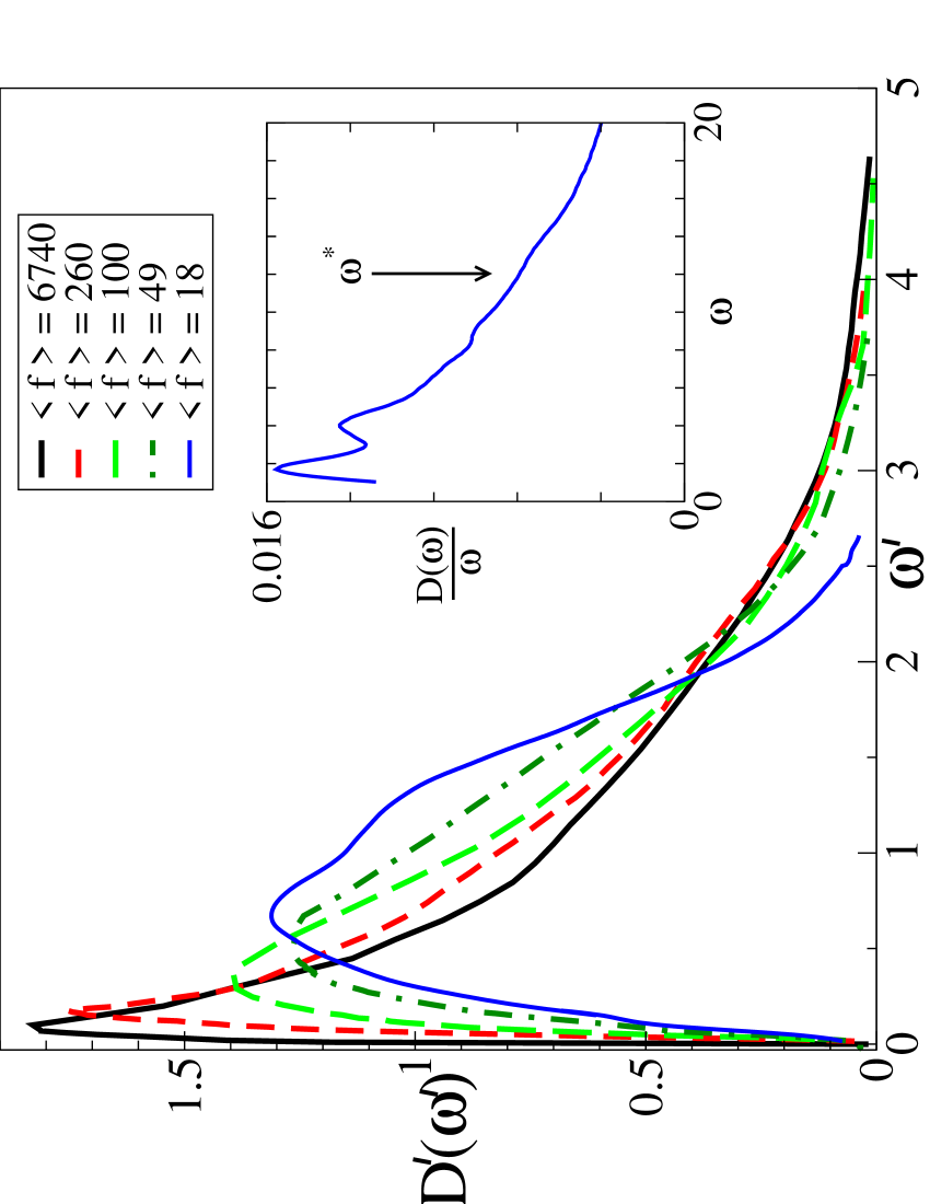
Figure 6: Densities of states $D^{\prime}(\omega^{\prime})\equiv\langle f\rangle D(\omega)$ vs. rescaled frequency $\omega^{\prime}=\omega/\langle f\rangle$ for different values of $\langle f\rangle$ in a system of $N=256$ particles. Inset: $D(\omega)/\omega$ vs. $\omega$ for $\langle f\rangle=18$.

From Fig.(6) we observe that: (i) there is an abundance of modes at low frequency. For all $\langle f\rangle$, $D^{\prime}(\omega^{\prime})$ increases rapidly from zero-frequency to reach a maximum at some frequency $\omega^{*}$, before decaying again. In the inset of Fig.(6), $D(\omega)$ is normalized by its Debye behavior $D_{d}(\omega)\sim\omega$ (plane waves would lead to a linear behavior of the density of states in two dimensions). No plateau can be detected at low frequency, we rather observe a peak in the quantity $D(\omega)/D_{d}(\omega)$, which appears at some frequency $\omega_{\scriptscriptstyle\rm BP}$ significantly smaller than $\omega^{*}$. This indicates that for our system size we do not observe any frequency range where plane waves dominate the spectrum. This is confirmed by inspection of the lowest-frequency modes, which appear to be quite heterogeneous. Two examples of lowest-frequency modes are shown in Fig.(7) for two values of $\langle f\rangle$. Those observations are consistent with the presence of barely stable soft modes in the spectrum.

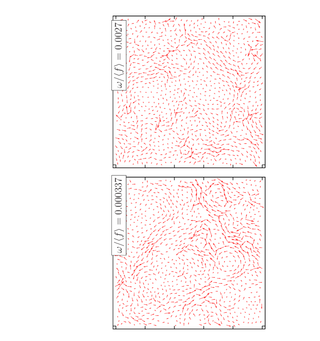
Figure 7: Examples of two lowest-frequency modes for $N=1024$ particles for $\langle f\rangle=7.8\times 10^{5}$ (left) and $\langle f\rangle=330$ (right).

(ii) There exists a characteristic frequency $\omega^{*}$ which scales with the pressure. We define $\omega^{*}$ as the frequency at which $D(\omega)$ is maximum: $D(\omega^{*})=D_{max}$. Fig.(8) shows the dependence of $\omega^{*}$ with the average force $\langle f\rangle$, where we observe the scaling:

$$\omega^{*}\sim\langle f\rangle^{1/2},$$ (21)

which holds well from the glass transition toward our densest packing, up to $\langle f\rangle=10^{4}$ for our system size. This scaling behaviour in the vibrational spectrum can be deduced from Eqs.(4,14) if marginal stability is assumed throughout the glass phase.

Both observations (i) and (ii) bring further support on the marginal stability of the meta-stable states, previously inferred from the microscopic structure.

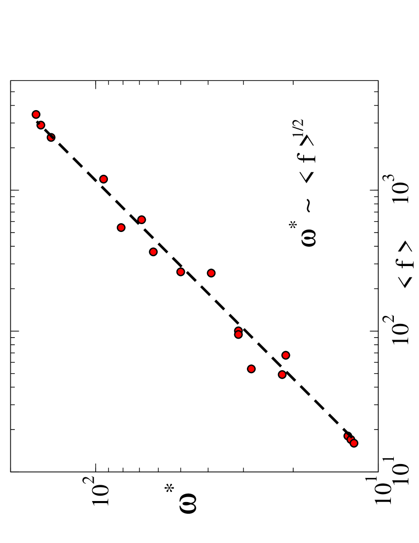
Figure 8: Characteristic frequency $\omega^{*}$ as defined in the text vs average force $\langle f\rangle$.

VI.2 Microscopic dynamics and normal modes

To study the microscopic dynamics, we project the dynamics on the normal modes and define for each frequency $\omega$:

$$C_{\omega}(t)=\langle~{}\langle\delta{\bf R}(t+t_{w})|\delta{\bf R}^{\omega}\rangle~{}.~{}\langle\delta{\bf R}(t_{w})|\delta{\bf R}^{\omega}\rangle~{}\rangle_{t_{w}},$$ (22)

where $|\delta{\bf R}(t)\rangle\equiv|{\bf R}(t)\rangle-|{\bf R}_{eq}\rangle$ is the displacement field around the configuration corresponding to the average particles position, and where the average is made on all time segments $[t_{w},t_{w}+t]$ entirely included in a meta-stable state.

If the projections of the dynamics were made on longitudinal plane waves rather than on normal modes, $C_{\omega}(t)$ would simply correspond to the de-correlation of the density fluctuations at some wave vector, which can be probed in scattering experiments. Examples of $C_{\omega}(t)$ for some low-frequency modes are presented in Fig.(9) at two different pressures, deep in the glass phase and in the super-cooled liquid. We observe damped oscillations for most of the spectrum.

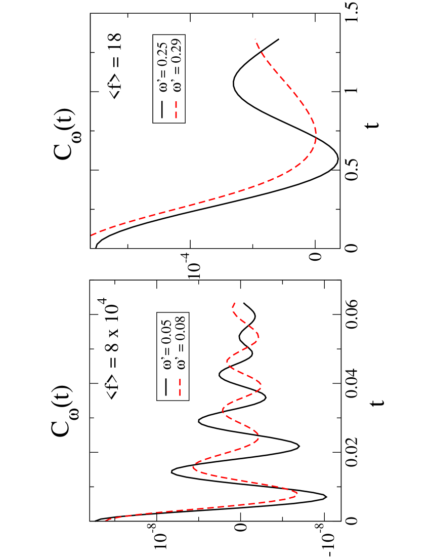
Figure 9: Examples of $C_{\omega}(t)/C_{\omega}(0)$ for low-frequency modes for two different average contact force $\langle f\rangle$, deep in the glass phase (left) and in the super-cooled liquid phase (right).

From $C_{\omega}(t)$, the amplitude $A(\omega)$ and the characteristic time $\tau(\omega)$ of the oscillations of a mode are readily extracted. The average square amplitude of the normal mode follows $\langle A^{2}(\omega)\rangle=C_{\omega}(0)$. We define the relaxation time scale $\tau(\omega)$ as the time at which $C_{\omega}(t)$ has decayed by some fraction $s$: $C_{\omega}(\tau(\omega))=sC_{\omega}(0)$. We have tried various definitions $s=0.3;0.5;0.9$ and found similar scaling for the dependence of $\tau(\omega)$ with $\omega$. In what follows we present the data with $s=0.9$ where our statistic is more accurate.

The dependence of these quantities with frequency are respectively shown in Fig.(10) for three meta-stable states at different pressure. Two configurations are in the glass phase and one in the super-cooled liquid phase. In all cases, these quantities were computed for each mode of the spectrum. We observe that the modes display weakly damped oscillations, whose amplitude and period follow:

$$\langle A^{2}(\omega)\rangle\sim\frac{1}{\omega^{2}},$$ (23)

$$\tau(\omega)\sim\frac{1}{\omega}.$$ (24)

These results hold true even for the low-frequency part of the spectrum, although more scattering is found there .

As a consequence, our computation of $D(\omega)$ gives a rather faithful distribution of relaxation time scales of the microscopic dynamics, supporting further the approximation we used to compute the free energy in Eq.(13), a priori strictly valid only at infinite pressure. This allows us to identify the peak apparent in the inset of Fig.(6) as the Boson Peak, which appears as a similar hump in Raman or neutron spectra in molecular liquids tao ; angell ; nakayama . Near the glass transition, this peak appears at a frequency significantly smaller than $\omega^{*}$, as shown by the inset of the Fig.(6) .

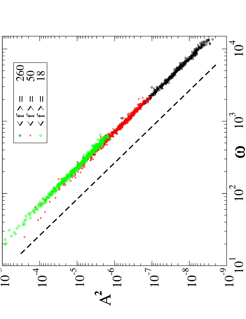
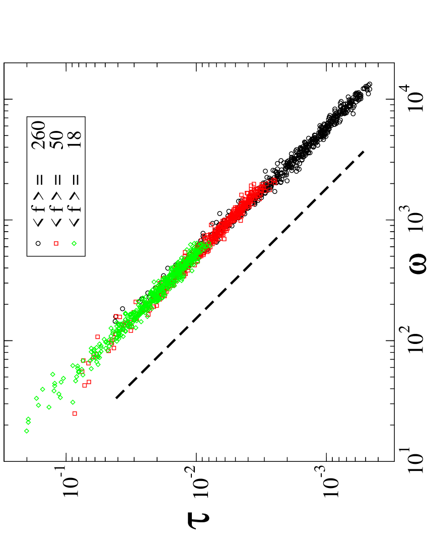
Figure 10: (a) Average squared amplitude of the modes $\langle A^{2}(\omega)\rangle$ vs $\omega$ at various packing fractions in a system of 256 particles, both in the glass phase ($\langle f\rangle=260$ and $\langle f\rangle=50$) or in the super-cooled liquid ($\langle f\rangle=18$). Each point corresponds to one mode. The dashed line corresponds to the fit $\langle A^{2}(\omega)\rangle\sim 1/\omega^{2}$. (b) Relaxation time $\tau(\omega)$ of each mode vs $\omega$ for the same packing fraction. The slashed line corresponds to the relation $\tau(\omega)\sim 1/\omega$.

VI.3 Mean squared displacement

In this section we use $D(\omega)$ to compute the mean square displacement around an equilibrium position inside a meta-stable state when $\langle f\rangle$ is varied. This quantity is directly related to the Debye-Waller factor accessible empirically with scattering experiments.

We define $\delta{\vec{R}_{i}}={\vec{R}_{i}}-{\vec{R}_{i}^{eq}}$, where ${\vec{R}_{i}^{eq}}$ is the average position of particles $i$ in a given meta-stable state as defined in Eq.(16). Assuming that the dynamics of different modes is independent, the fluctuations of particles positions $\langle{\delta\vec{R}_{i}}^{2}\rangle$ can be written as a sum of the fluctuation of all modes:

$$\langle{\delta\vec{R}_{i}}^{2}\rangle=\sum_{\omega}\langle A^{2}(\omega)\rangle\langle{\delta\vec{R}_{i}(\omega)}^{2}\rangle$$ (25)

where $A^{2}(\omega)$ is the average square amplitude of the amplitude of the mode $\omega$ and ${\delta\vec{R}_{i}(\omega)}$ is the displacement of particle $i$ for the mode $\omega$. We then average on all particles and define $\langle\delta\vec{R}^{2}\rangle=1/N~{}\sum_{i}\langle{\delta\vec{R}_{i}}^{2}\rangle$ where $N$ is the system size. Using the modes normalization $\langle{\delta\vec{R}_{i}(\omega)}^{2}\rangle_{i}=1/N$ and applying Eqs.(24) lead to:

$$\langle{\delta\vec{R}}^{2}\rangle\sim\int_{0}\frac{D(\omega)}{\omega^{2}}d\omega\geq\int_{\omega^{*}}\frac{D(\omega)}{\omega^{2}}d\omega.$$ (26)

The inequality accounts for the modes with frequency between $\omega=0$ and $\omega^{*}$ that we have neglected. Accounting for those modes would not change our conclusion as long as the soft modes density grows sub-linearly at low frequency. As can be checked for the square lattice, $D(\omega)$ reaches a typical value $1/\sqrt{k}$ ($\sim 1/\langle f\rangle$ for hard spheres) for $\omega\geq\omega^{*}$. This is more generally true for amorphous packing, as proven in matthieu1 . Using this fact, the last integral is dominated by the lowest bound and one gets:

$$\langle{\delta\vec{R}}^{2}\rangle\geq\frac{D(\omega^{*})}{\omega^{*}}\sim\langle f\rangle^{-3/2}\sim h^{3/2}$$ (27)

which holds in any dimension $d\geq 2$ (with corrections of order $h^{2}\log N$ for $d=2$ due to plane waves). We have used the scaling of the frequency scale $\omega^{*}$ confirmed in Fig.(8). In crystals, the fluctuations around a particle position is of the order of the inter-particle gap $h$: $\langle\delta{\vec{R}}^{2}\rangle\sim h^{2}$ (with $\log N$ corrections in two dimensions). Eq.(27) shows that, near maximum packing, the amplitude of particles motions is infinitely smaller in the crystal than in the glass. Because of the marginal stability of the glass, these fluctuations have an anomalous scaling with the packing fraction.

To check numerically this prediction, we consider various meta-stables states. In each of them, we measure $\vec{R}_{i}^{eq}$ and the mean square displacement around the equilibrium position: $\langle\delta\vec{R}^{2}\rangle=\langle 1/N~{}\sum_{i}\delta\vec{R}_{i}^{2}(t)\rangle_{t_{1}}$, where the average is made on the time interval $t_{1}$. Fig.(11) show this quantity for various packing fraction. Our numerical result agrees well with our prediction $\langle\delta\vec{R}^{2}\rangle\sim\langle f\rangle^{-3/2}\sim h^{3/2}$ throughout the glass phase.

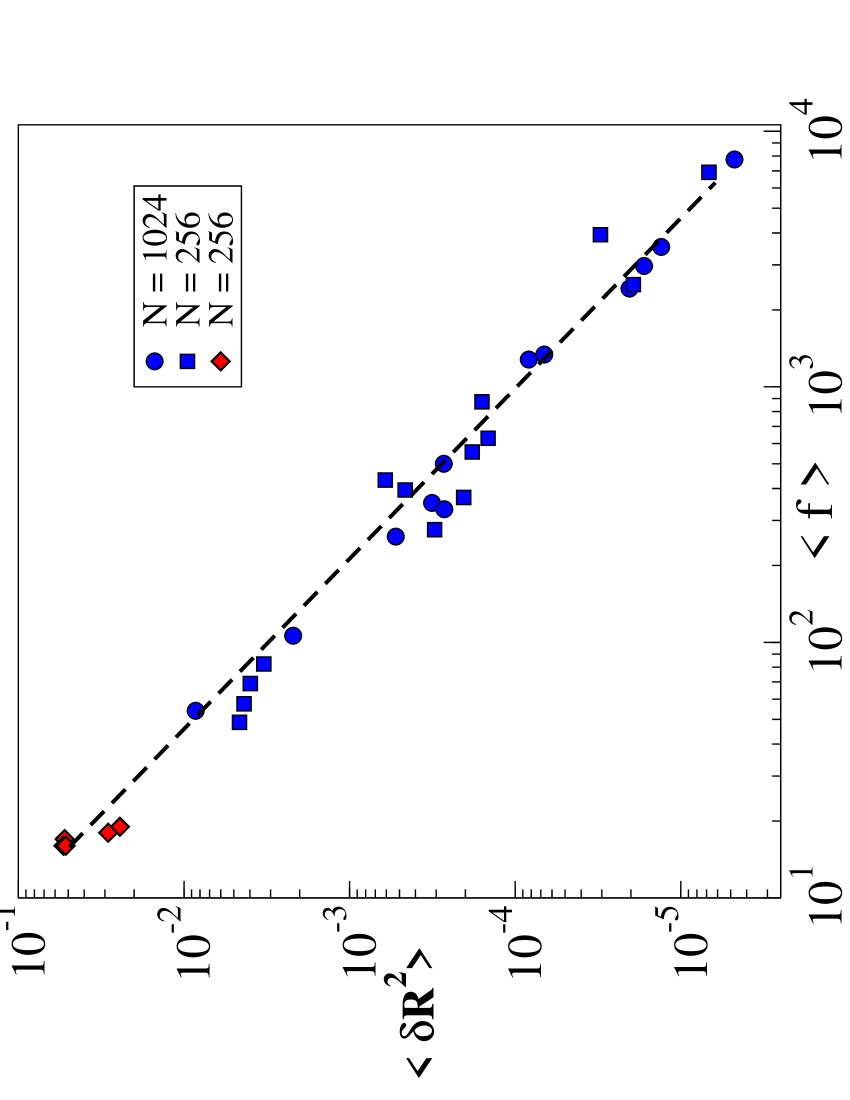
Figure 11: Mean square displacement $\langle\delta\vec{R}^{2}\rangle$ versus average contact force $\langle f\rangle$ for $N=1024$ (circles) and $N=256$ (squares) particles. Diamonds correspond to the super-cooled liquid phase and were computed for a system with $N=256$ particles. Slashed line corresponds to the best fit agreeing with our prediction $\langle\delta\vec{R}_{i}^{2}\rangle\sim\langle f\rangle^{-3/2}$.

VII $\alpha$-relaxation

One long-lasting challenge in our understanding of the glass transition is the elaboration of a spatial description of activated events, the rare and sudden rearrangements of particles corresponding to jumps between meta-stable states. These events are collective rearrangements of particles, but the cause and the nature of this collective aspect is unknown. Our observation that the glass structure is marginally stable suggests that the softest, barely stable modes may play a key role in the activated events that relax the structures. In what follows we investigate this possibility by projecting the sudden rearrangements on the normal modes of the free energy.

VII.1 Aging

During aging, sudden rearrangements, or “earthquakes”, appear as drops in the self scattering function, see Fig.(2-a). Such earthquakes correspond to collective motions of a large number of particles, and have been observed in various other aging systems, such as colloidal paste or laponite duri , and in Lennard-Jones simulations lapo ; kb ; heuer . Even for our largest numerical box of $N=1024$ particles, deep in the glass phase these events generally span the entire system. Examples of earthquakes in real space are shown in Fig.(14).

To analyze these displacement fields, we measure the average particle positions and the contact network in the meta-stable state prior to the earthquake, and compute the normal modes of the free energy. We also compute the earthquake displacement $|\delta{\bf R}^{e}\rangle$ defined as a difference between the average particles position in two successive meta-stable states $l$ and $m$: $|\delta{\bf R}^{e}\rangle\equiv|{\bf R}^{m}\rangle-|{\bf R}^{l}\rangle$. We then project $|\delta{\bf R}^{e}\rangle$ on the normal modes and compute $c_{\omega}\equiv\langle\delta{\bf R}^{e}|\delta{\bf R}^{\omega}\rangle/\langle\delta{\bf R}^{e}|\delta{\bf R}^{e}\rangle$. The $c_{\omega}$’s satisfy $\sum_{\omega}c_{\omega}{}^{2}=1$ since the normal modes form a unitary basis. To study how the contribution of the modes depends on frequency, we define:

$$g(\omega)=\langle c_{\omega}{}^{2}\rangle$$ (28)

where the average is made on a small segment of frequencies $[\omega,\omega+d\omega]$. Fig.(12-a) shows $g(\omega)$ for the earthquake shown in Fig.(2-a). The average contribution of the modes decreases very rapidly with increasing frequency, and most of the displacement projects on the excess-modes present near zero-frequency. This supports that the free energy barrier crossed by the system during a rearrangement lies in the direction of the softest degrees of freedom.

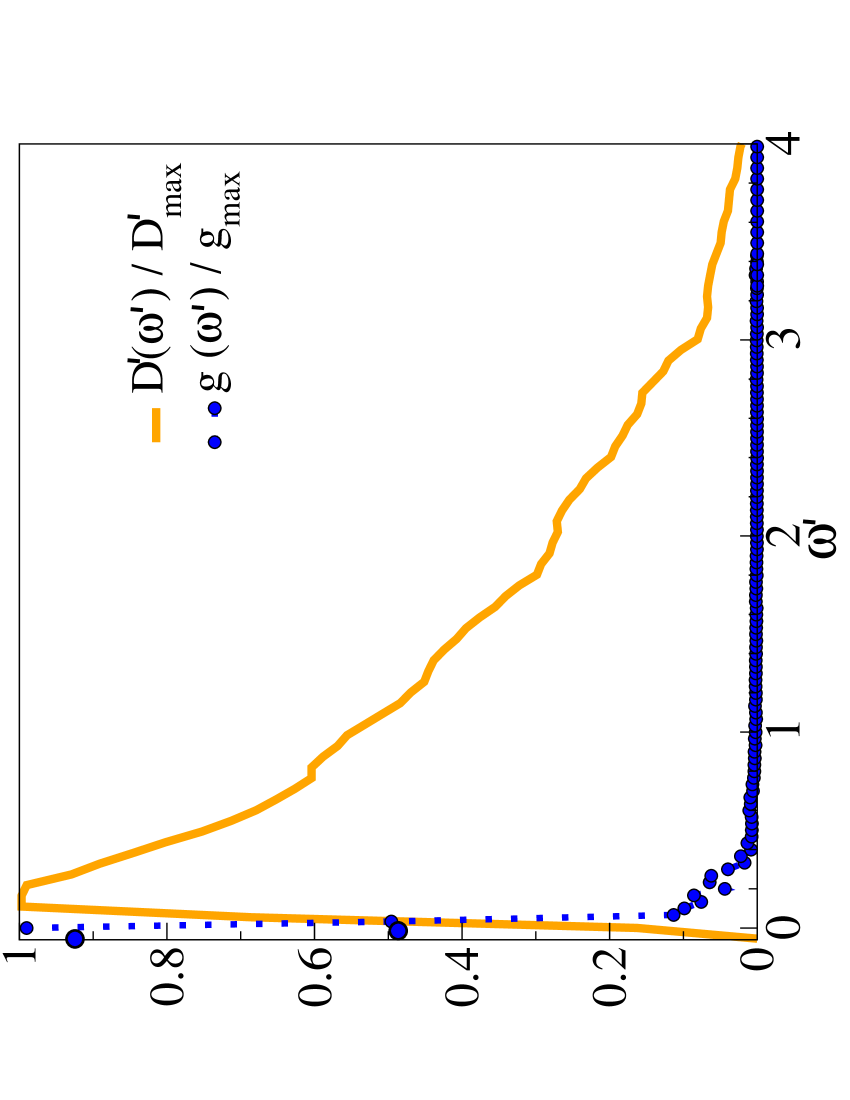
Figure 12: Straight curve: $D^{\prime}(\omega^{\prime})/D^{\prime}_{max}$ vs. $\omega/\langle f\rangle$. Both $D(\omega)$ and $\langle f\rangle$ are computed in the meta-stable state prior to the earthquake shown in the Fig.(2-a). Dotted curve: $g(\omega)$ as defined in the text re-normalized by its maximum value $g(\omega^{\prime})/g_{max}$ vs. $\omega/\langle f\rangle$. This figure has been originally published in the reference “Heterogeneous dynamics, marginal stability and soft modes in hard sphere glasses”, J. Stat. Mech., L08003, (2007), by C. Brito and M. Wyart.

To make this observation systematic, introduce the label $i$ to rank the $c$’s by decreasing order: $c_{1}>c_{2}...>c_{2N}$. We then defined a $k_{1/2}$ such that:

$$\sum_{i=1}^{k_{1/2}}c_{i}^{2}\equiv 1/2$$ (29)

Physically, $k_{1/2}$ is the minimum number of modes necessary to reconstruct $50\%$ of the displacements relative to the earthquake. Fig.(13) shows $F_{1/2}\equiv k_{1/2}/(2N)$ for the 17 cracks studied and indicates that $0.2\%<F_{1/2}<2\%$ for all the events studied throughout the glass phase. We thus systematically observe that the extended earthquakes correspond to the relaxation of a small number of degrees of freedom, of the order of $1\%$ of the modes of the system.

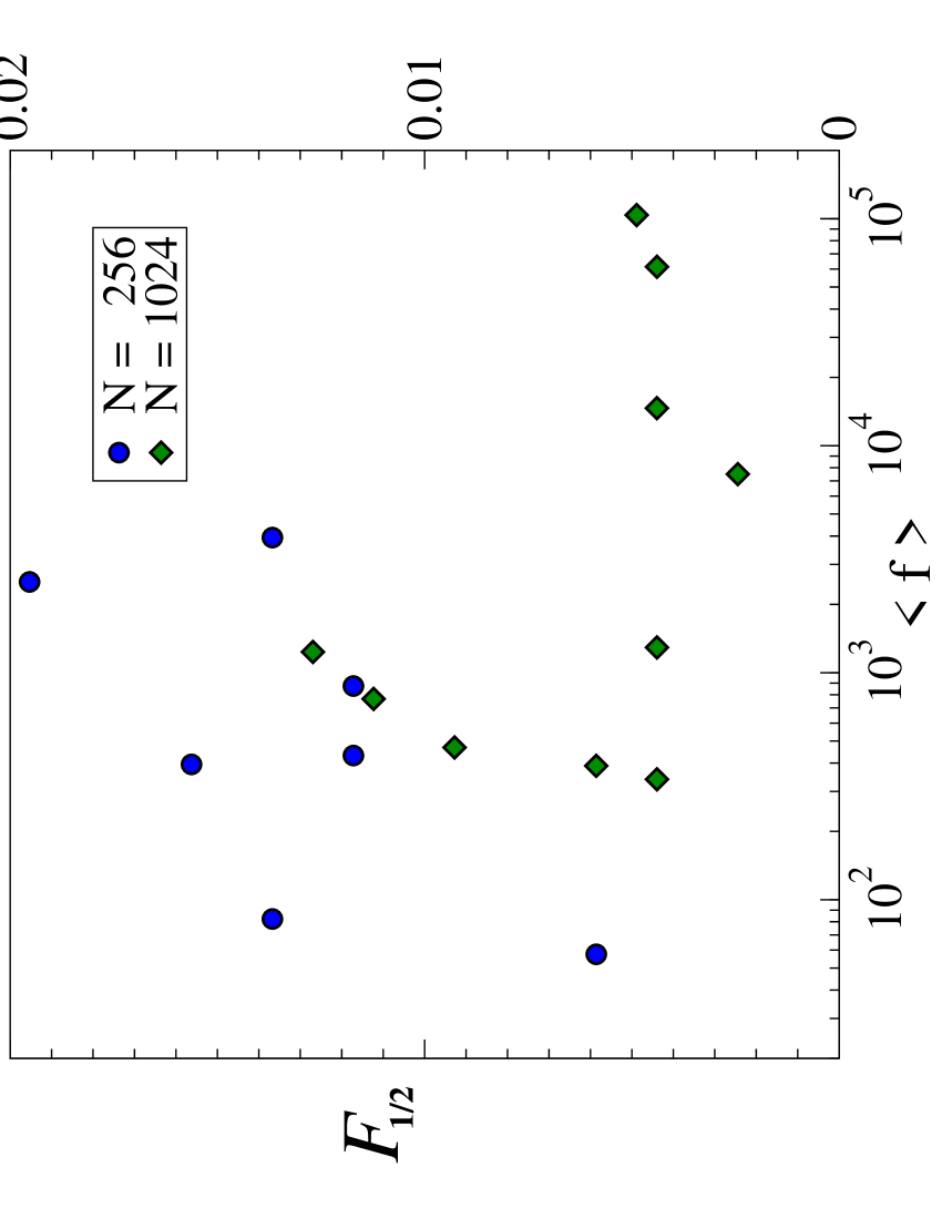
Figure 13: $F_{1/2}$ vs. $\langle f\rangle$ for $N=256$ (circles) and $N=1024$ (diamonds) particles. This figure has been originally published in the reference “Heterogeneous dynamics, marginal stability and soft modes in hard sphere glasses”, J. Stat. Mech., L08003, (2007), by C. Brito and M. Wyart.

In Fig.(14) we illustrate the spatial consequence of our analysis. Two examples of earthquakes at different packing fractions are compared with the linear superposition of the $1\%$ of the modes that contribute most to them. The similarity is striking: the complexity of the structural relaxation is indeed contained in the soft degrees of freedom of the system, along which yielding occurs. Thus, in this regime only a small fraction of the degrees of freedom of the system participates in the relaxation of the structure.

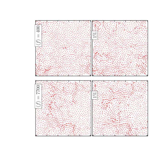
Figure 14: Above: two examples of earthquakes in the glass phase for different average contact force $\langle f\rangle$ for $N=1024$ particles. Displacements were multiplied by four for visibility. Below: projection of earthquakes on the $1\%$ of the normal modes that contribute most to them.

VII.2 Structural Relaxation in the equilibrated super-cooled liquid

We equilibrate the system for a range of density $0.77\leq\phi\leq 0.786$. Also in this regime, the dynamics is heterogeneous in space and in time and sudden rearrangements still occur on time scales of the order of $\tau$ kob . An example of this rearrangement, that can be identified as a drop in the self-scattering function, is shown in the Fig.(2-b). In real space, this displacement corresponds to a collective event, as one can observe in the examples of the Fig.(16-left) and Fig.(18-above). To study these events in an equilibrated super-cooled liquid, we extend the procedure used in the aging regime: we identify the meta-stable states visited by the dynamics and compute their averaged configuration. We then define the normal modes in the meta-stable state and the displacement field corresponding to the relaxation events. For each relaxation event, we compute $F_{1/2}$.

We start with a system with $N=64$ particles. For each packing fraction, $F_{1/2}$ is computed for six relaxation events. Then this quantity is averaged on all events. The result of these $\langle F_{1/2}\rangle$ are shown in Fig.(15) as a function of the packing fraction. We find that $\langle F_{1/2}\rangle\leq 5\%$ for all $\phi$ studied, supporting that only a small fraction of the low-frequency modes contribute to the structural relaxation events also in this region of the super-cooled liquid. This fraction decays significantly as $\phi$ get closer to $\phi_{0}$, suggesting a rarefaction of the number of directions along which the system can yield near the glass transition. Fig.(16) exemplifies this conclusion: for this particular case, the relaxation event shown on the left projects almost entirely on one normal mode, shown on the right in this same figure. This mode turns out to be the lowest-frequency normal mode of the free energy.

To study finite-size effects, we measure $F_{1/2}$ for twelve relaxation events at each of the five packing fraction using $N=256$ particles. Results are shown in Fig.(15). Finite size effects are present, and $\langle F_{1/2}\rangle$ appears to be roughly $0.5\%$ higher in the larger system for all packing fractions. Most of this difference in behavior is explained by the observation that the glass transition occurs at smaller packing fraction in the $N=64$ system, as previously observed yy . The inset of Fig.(17) shows that this is the case in our system as well. If $\langle F_{1/2}\rangle$ is plotted as a function of relaxation time, as in Fig.(17), the curves become similar for the two systems and $\langle F_{1/2}\rangle$ is systematically smaller for a system with $N=256$ particles. Thus, even for larger systems, collective rearrangements relaxing the system are “soft”: they project mostly into a small portion of the vibrational spectrum. We verify spatially this observation in Fig.(18). Three examples of relaxation events at different packing fractions are compared with the vector field which is a linear superposition of the modes that contribute most to them. This relation between soft modes and relaxation has been recently supported by the observation that regions where structural relaxation is likely to occur, said to have a high “propensity”, also display an abundance of soft modes Harrowell_NP .

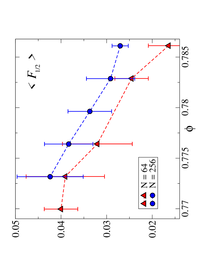
Figure 15: $\langle F_{1/2}\rangle$ vs $\phi$ for two different system sizes. This figure has been originally published in the reference “Heterogeneous dynamics, marginal stability and soft modes in hard sphere glasses”, J. Stat. Mech., L08003, (2007), by C. Brito and M. Wyart.

Figure 16: Left: displacement field for a system with $N=64$ particles corresponding to a relaxation event. Arrows were multiplied by $1.2$. Right: normal mode that contains $80\%$ of the projection of the real displacement field. This normal mode has the lowest frequency of the spectrum. This figure has been originally published in the reference “Heterogeneous dynamics, marginal stability and soft modes in hard sphere glasses”, J. Stat. Mech., L08003, (2007), by C. Brito and M. Wyart.

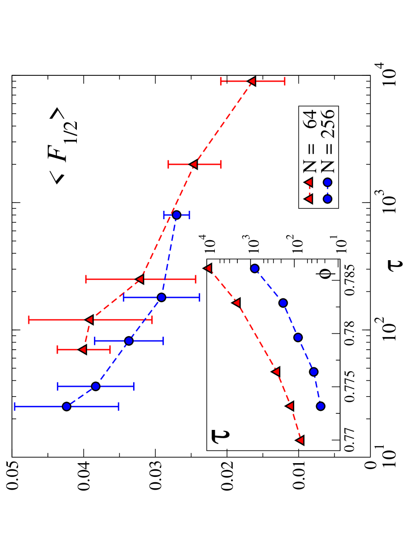
Figure 17: $\langle F_{1/2}\rangle$ vs $\tau$. Inset: $\alpha$-relaxation time vs $\phi$. System sizes are indicated in the legend. This figure has been originally published in the reference “Heterogeneous dynamics, marginal stability and soft modes in hard sphere glasses”, J. Stat. Mech., L08003, (2007), by C. Brito and M. Wyart.

Interestingly, the soft modes that characterize marginally stable structures are in general rather extended objects, as can be observed from the examples presented here. Theoretically this is what one expects both in the square lattice, as justified by Eq.(3), and in amorphous packing matthieu1 ; matthieu2 . In this light it does not seem surprising that activated events are collective.

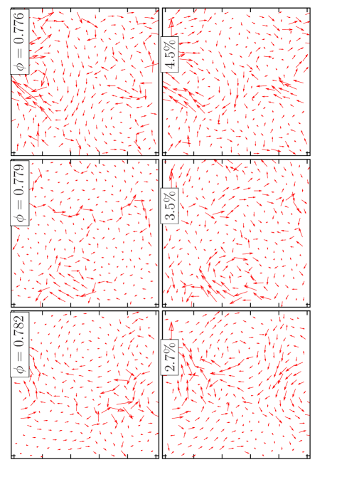
Figure 18: Above: Relaxation events in the super-cooled liquid for different $\phi$, indicated in the figure, and $N=256$ particles. Displacement fields are rescaled by 4, 1.5 and 1.2 respectively for visibility. Below: projection of the relaxation events on the normal modes that contribute the most. The fraction of the total number of modes used is indicated in each figure, and corresponds to the fraction necessary to recover $50\%$ of the relaxation event. As indicated in Fig.(15), this fraction of modes tend to increase as $\phi$ decreases.

VIII A geometric interpretation of pre-vitrification

VIII.1 Pre-vitrification

We have shown, both from its microscopic structure and microscopic dynamics, that the hard sphere glass lies close to marginal stability. In this section we propose an explanation for this observation. This requires a single assumption, namely that the viscosity increases very rapidly when meta-stable states appear in the free energy landscape. In the logarithmic representation of the plane coordination vs the typical gap between particles in contact $(\delta z,h)$, there exists a line, corresponding to the equality of Eq.(14), which separates a region where configurations are stable and unstable, as sketched in Fig.(19). At any packing fraction $\phi$, equilibrium configurations correspond to a point in the $(\delta z,h)$ phase diagram. As $\phi$ is varied equilibrium states draw a line in this plane, represented by the dashed line (red online) in Fig.(19). At low $\phi$, gaps among particle are large and configurations visited are unstable. As $\phi$ increases, the gaps narrow, and configurations become eventually stable. This occurs at some $\phi_{onset}$ when the equilibrium line crosses the marginal stability line. At larger $\phi$, the viscosity increases sharply, so that on our numerical time scales equilibrium cannot be reached deep in the regions where meta-stable states are present. As a consequence, the system falls out of equilibrium at some $\phi_{0}$ close but larger than $\phi_{onset}$. Configurations visited must therefore lie close to the marginal stability line, as represented by the dotted line in Fig.(19), since more stable, better-coordinated configurations cannot be reached dynamically.

In this view, $\phi_{onset}$ corresponds to the onset temperature, where activation sets in and the dynamics becomes intermittent. When intermittency appears, the $\alpha$-relaxation time scale $\tau$ is still limited, and has increased roughly of one order of magnitude from the liquid state. This is consistent with the observation that the configurations we probed in the super-cooled liquid, for which $\tau$ is larger but still limited, are already stable: the free energy expansion has in general a positively-defined spectrum. Note that at $\phi_{onset}$, $\delta z\neq 0$, and the characteristic length of the soft modes $l^{*}$ is finite. We think of those modes as involving a few tens of particles.

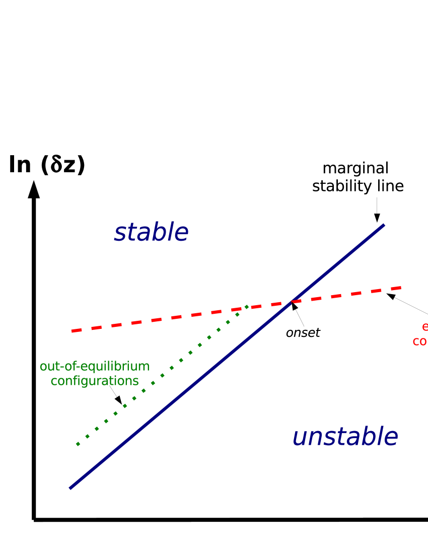
Figure 19: Phase diagram for the stability of hard sphere configurations, in the coordination $\delta z$ vs average gap $h$ plane. The marginal stability line delimits stable and unstable configurations. The dashed line correspond to equilibrium configurations for different $\phi$. As $\phi$ increases, $h$ decreases and the two lines eventually meet. This occurs at the onset packing fraction $\phi_{onset}$, where dynamics become activated. At larger $\phi$, viscosity increases sharply as configurations visited become more stable. For a finite quench rate the system eventually falls out of equilibrium. More stable and more coordinated regions cannot be reached dynamically, and as $\phi$ is increased further, the system lives close to the marginal stability region, as indicated in the dotted line. The location of the out-of-equilibrium trajectory depends on the quench rate. In the limit of very rapid quench, the out-of-equilibrium line approaches the marginal stability line.

VIII.2 Ideal glass and random close packing

To put our work in a broader context it is useful to think about the phase diagram of Fig.19 with an extra dimension added. For any configuration one can associate the packing fraction $\phi_{c}$ corresponding to the jammed packing that would be obtained after a rapid compression speedy ; kurchan ; zamponi . At equilibrium $\phi_{c}$ is an increasing function of pressure donev ; berthier . In the three-dimensional phase diagram $(h,\delta z,\phi_{c})$, marginality is now represented by a surface. Its main feature, the scaling relation between coordination and typical gaps expressed in Eq.(14), holds irrespectively of the value of $\phi_{c}$ according to our theoretical analysis, in agreement with the data presented in Fig.(5). Marginality and related properties are therefore adequately discussed in the more simple two-dimensional phase diagram presented in Fig.19. Some other aspects of the dynamics and thermodynamics of hard spheres nevertheless benefit from introducing the extra dimension $\phi_{c}$.

Ideal glass: For molecular glasses the presence of an ideal glass transition where the configurational entropy vanishes at finite temperature has been proposed and is still debated wolynes ; stillinger . For hard spheres this view implies that the viscosity diverges at some finite $h>0$ kurchan ; zamponi , for which the equilibrium curve $\phi_{c}(h)$ reaches a constant value. Our work does not address the issue of the existence of an ideal glass, but it supports that if it exists, it is not responsible for the slow-down of the dynamics in the pre-vitrification region we can access empirically, neither in the aging regime we could observe in the glass, since such a scenario would not explain the marginal stability of the microscopic structure we observe. Some authors have used diverging fits of the relaxation time to argue in favor of the opposite view berthier . Nevertheless, establishing the existence of an actual divergence from such fits is questionable even in molecular liquids dyre where the number of decades of viscosities accessible is two to three times larger.

Random Close Packing: Empirically it is observed that for various protocols of compression (such as pouring metallic balls in a container), the final packing fraction obtained is $\phi_{c}\approx 0.64$ for mono-disperse hard spheres. This fact can be expressed as follows: for each protocol one can associate a line $\delta z(h),\phi_{c}(h)$ characterizing the configurations visited during compression. Isostaticity implies $\delta z\rightarrow 0$ as $h\rightarrow 0$. Furthermore, for a wide class of protocols $\phi_{c}(h)\rightarrow 0.64$ as $h\rightarrow 0$. The explanation for this observation is debated kurchan . An interesting hypothesis is that $\phi_{c}\approx 0.64$ corresponds to the limit reached by infinitely rapid compressions. If typical protocols are fast in comparison with the relevant time scales of the dynamics, they should generate packings with a similar packing fraction.

IX Conclusion

We conclude by a brief summary of our results and a few remarks. We have derived a geometric criterion for the stability of hard sphere configurations, and we have shown that in a hard sphere glass this bound is nearly saturated. This supports that pre-vitrification occurs when the coordination is sufficiently large to counter-balance the destabilizing effect of the compression in the contacts. Nearly unstable modes are collective displacement fields, whose spatial extension is governed by the coordination. Once meta-stable states appear in the free energy, activation occurs mostly along a small fraction of these soft modes. This observation supports that these modes are the elementary objects to consider to describe activation. It also implies that structural relaxation must be cooperative, since the soft degrees of freedom are collective.

We have observed that less and less modes participate to the structural relaxation as the packing fraction increases near $\phi_{onset}$. It is tempting to speculate that, as the number of degrees of freedom allowing relaxation is reduced, the size of the cooperatively rearranging regions grows to eventually saturate at the extension of the softest modes $l^{*}$. Nevertheless, a quantitative description of the relationship between soft modes and dynamical length scale remains to be built and tested. Other factors, such as the possible presence of locally favored structure of high coordination or some other spatial heterogeneities of the structure, may also have to be taken into account.

Our analysis of the structural relaxation at equilibrium applies to the pre-vitrification region, corresponding to the intermediate viscosities that can be probed numerically. Similar time scales are accessible experimentally in shaken granular matter and colloidal glasses. Our work does not address the behavior of the equilibrium dynamics for very large packing fraction. As a consequence, it is possible that at much larger viscosities than those we probed, in particular near the glass transition in molecular liquids, our observations on the nature of the structural relaxation may not apply, and soft modes may play no role in the dynamics. Nevertheless several observations support that soft modes and dynamics are related even for those large viscosities. In particular, the intensity of the boson peak, which indicates the presence of soft modes in the spectrum, strongly correlates with the glass fragility novikov , a fact which is not captured by current theories of the glass transition.

Finally, our geometric approach to pre-vitrification is consistent with Goldstein goldstein views, who proposed 40 years ago that the glass transition is related to the emergence of meta-stable states in the energy landscape. Other more recent descriptions of the glass transition, such as the mode coupling theory (MCT) of liquids sjorgen , make a similar prediction wolynes ; parisi ; laloux ; isabelle , and it is interesting to compare this approach to ours. Here we indicate several differences and analogies in the respective conclusions: (i) in MCT the predicted location of the elastic instability corresponds to the onset packing fraction brumer . This is consistent with our observation that when the dynamics becomes intermittent ($\phi\geq\phi_{onset}$), the configurations visited have in general a positively defined spectrum, displaying no unstable modes. This is also supported by previous results showing that the dynamics is dominated by activation in this parameter range activation . Nevertheless, MCT predicts diverging time scales sjorgen and dynamical length scales bb at the onset packing fraction, which are not observed. Fitting empirical data with such divergences hans leads to a critical packing fraction $\phi_{MCT}$ significantly larger than $\phi_{onset}$. The interpretation of the extra fitting parameter $\phi_{MCT}$, and its relation with the free energy landscape, is at present unclear. (ii) In MCT the dynamics is computed via a resummation of a perturbation expansion in the non-linear interaction among modes, around a point where plane waves are un-coupled. In our case, we use a variational argument matthieu1 ; matthieu2 to capture the properties of the linear soft modes whose stability is at play. This argument applies as well in covalent these_matt and attractive glasses these_matt ; ning2 . This leads to an estimation of a length scale $l^{*}$ characterizing soft modes, which depends on the coordination. This length scale has not yet found a correspondence within MCT, where non-trivial length scales appear from the dynamics bb but diverge near the elastic instability, unlike $l^{*}$. (iii) In our approach, the key microscopic parameters determining the location of the transition are coordination and pressure. In MCT, an important parameter is the area under the first peak of the pair correlation function lapo . These two views bear similarities, as the later quantity can be considered as a rough measure of coordination. It remains to be seen if MCT can capture the critical behavior of the marginal stability line observed at very large pressure. Exploring this possibility may clarify the physical meaning of the approximations that characterize MCT.

Appendix A Determination of the rattlers

Near maximum packing, a few percents of the particles are trapped in a large “cages” on which they apply a minuscule force in comparison to the typical contact forces in the system. Such particles, called rattlers, do not participate to the rigidity of the structure: if removed, stability is still achieved. When we compute e.g. the coordination of the microscopic structure, we do not take these particles into account.

To identify rattlers we measure the average number of shocks per contact for each particle. We compute how many shocks $n_{shoc}$ and how many contacts $n_{c}$ each particle has during the interval of time $t_{1}$ and define: $f^{*}=n_{shoc}/n_{c}$ if $n_{c}\geq 2$ and $f^{*}=0$ otherwise. This quantity is normalized by the average number of shocks per contact that all particles have during $t_{1}$: $F^{*}=N_{shoc}/N_{c}$, where $N_{shoc}$ in the total number of shocks and $N_{c}$ is the total number of contacts in the system. We then plot the distribution of $f^{*}/F^{*}$ for different packing fractions, Fig.(20). At large $\langle f\rangle$, we observe the emergence of a peak near zero. When $\langle f\rangle$ is intermediate, $\langle f\rangle=5.2\times 10^{3}$ and $\langle f\rangle=9.2\times 10^{2}$, the peak vanishes. This peak corresponds to the rattlers. In this work we consider that all particles for which $f^{*}/F^{*}\leq 2\%$ are rattlers. This criterion is represented by the arrow in the inset of the Fig.(20).

Figure 20: Histogram of the distribution of $f^{*}/F^{*}$ (see definition in the text) for various average force.

To check the robustness of our results, we test if the relation between the excess of coordination $\delta z$ and the average force $\langle f\rangle$ depends on this criterion. We vary the threshold bellow which we consider a particle as a rattler and plot in the Fig.(21) the comparison between 3 different criteria: $f^{*}/F*\leq 0.01\leq 0.02\leq 0.05$. We observe that relation $\delta z=A_{1}\langle f\rangle^{-1/2}$ holds irrespectively of the criterion. It fails when the rattlers are not removed of the analysis. In this case, for high values of $\langle f\rangle$ one finds $\delta z<0$.

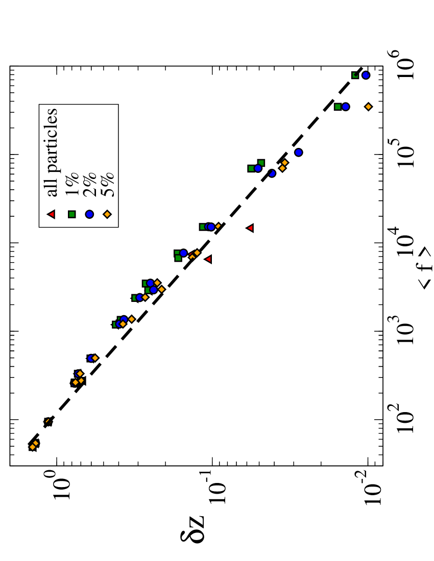
Figure 21: $\delta z$ vs $\langle f\rangle$ for 3 different criteria of definition of rattlers as explained in the text. The legend “all particles” indicates that no rattlers are excluded for this measure. Dotted curve: fit of the relation $\delta z=A\langle f\rangle^{-1/2}$.

Appendix B Persistence of the normal modes in a meta-stable state

Here we show that our numerical computation of the normal modes is robust to different choices of time intervals, as long as they lie in the same meta-stable state. To achieve that we compute the normal modes for two distinct, non-overlapping time-intervals. $|\delta{\bf R}_{t_{a}}^{\omega}\rangle$ denotes the normal modes of frequency $\omega$, computed on some time interval labeled $t_{a}$. We then compute the matrix of scalar product:

$$C_{\omega,\omega^{\prime}}=\langle\delta{\bf R}_{t_{a}}^{\omega}|\delta{\bf R}_{t_{b}}^{\omega^{\prime}}\rangle.$$ (30)

If the two sets of normal modes are identical, $C$ is the identity matrix. In general this must not be exactly true, as shown in Fig.22, since our protocol requires time-averaging and is therefore noisy to some extent, and also because some non-trivial dynamics may still occur within meta-stable states. Our observations below show that those effects are small, even if the two time-intervals considered are separated by a time scale of the order of the life-time of meta-stable states. To quantify the difference between $C$ and the identity matrix, we follow the procedure we used before to compare a relaxation event to the normal modes of the structure. We define $F_{1/2}(\omega)$ as the minimal fraction of normal modes computed on $t_{b}$ sufficient to represent $50\%$ of a normal model of frequency $\omega$ computed on $t_{a}$. We then define $\langle F_{1/2}\rangle$ as the average of $F_{1/2}(\omega)$ on the 20 lowest-frequency modes computed on $t_{a}$. $\langle F_{1/2}\rangle$ is $1/2N$ if $C$ is the identity matrix, and should be small if our procedure is robust to different choice of time-interval. This is indeed the case: in the super-cooled liquid ($\langle f\rangle=18$) we find $\langle F_{1/2}\rangle=0.4\%$, which is small for all practical purposes discussed in this article. For this measure the time intervals lasted $t_{1}=500\tau_{c}$, and the time separation between $t_{a}$ and $t_{b}$ was $10^{4}\tau_{c}$, which is of the order of the relaxation time $\tau\approx 3\times 10^{4}\tau_{c}$. For the glass ($\langle f\rangle=6700$) $F_{1/2}(\omega)$ is close to $1/2N$, as is obvious from Fig.22.

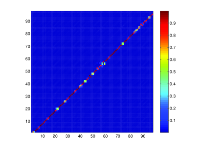
Figure 22: Matrix of scalar product $C$ as defined in the text for the 100 lowest-frequency modes for $N=256$. The colorbar indicates the value of the scalar product. Time intervals lasted $t_{1}=500\tau_{c}$. Left: $\langle f\rangle=6700$. The intervals $t_{a}$ and $t_{b}$ are separeted by $10^{5}\tau_{c}$. Right: $\phi=0.782$. The intervals $t_{a}$ and $t_{b}$ are separeted by $10^{4}\tau_{c}$, which is of the order of the relaxation time.

List of Figures

1. 1 Square lattice of springs with a density per particle $\delta z$ of additional diagonal springs, represented in dotted lines. $l^{*}\sim\sigma/\delta z$ is the typical dimensionless distance of the segments contained between two diagonal springs on a given row or column. The arrows represent the longitudinal mode of wavelength $\sim l^{*}$ of such a segment: $\delta{\vec{R}_{i}}\sim\sin(\pi i\sigma/l^{*}){\vec{e}_{x}}$, following the notation introduced in the text. The dashed line exemplifies the deformation of a spring transverse and directly connected to the segment considered, it is elongated by the longitudinal vibration of this segment. When the pressure is positive and contacts are under compression, this elongation lowers the energy contained in those springs. This leads to an elastic instability when $\delta z$ becomes smaller than a quantity proportional to the square root of the contact strain, of order $f/k\sigma$.
2. 2 Examples of $C(\vec{q},t,t_{\omega})$ as defined in Eq.(15) vs $t$ (a) in the glass and (b) in the super-cooled liquid.
3. 3 Contact forces for $N=256$, $\langle f\rangle=6740$ and $t_{1}=10^{4}$ time steps. Points represent particles centers. Contact forces are sketched by line segments which link particles that are in contact. The width of these segments is proportional to the force amplitude. This figure has already been published in the reference “On the rigidity of hard sphere glass near random close packing”, Europhyscis Letters, v 76, 149-155 (2006) by C. Brito and M. Wyart and it is reproduced here under permission of the Institute of Physics Publishing (IOP).
4. 4 Log-log plot of the amplitude of the contact force vs the gap between the particles for different values of $\langle f\rangle$ in a system with $N=256$ particles. Each point corresponds to a pair of numbers ($f_{ij},\langle h_{ij}\rangle$) that characterizes a pair of particles in contact. The slashed line is a fit of the theoretical relation predicted in Eq.(11). This figure has already been published in the reference “On the rigidity of hard sphere glass near random close packing”, Europhyscis Letters, v 76, 149-155 (2006) by C. Brito and M. Wyart and it is reproduced here under permission of the Institute of Physics Publishing (IOP).
5. 5 Log-log plot of $\delta z$ vs $\langle f\rangle$ for $N=256$ or $N=1024$ particles. Each circle correspond to one meta-stable state in the glass phase, whereas diamonds correspond to averaged quantity among 11 meta-stable states in the super-cooled liquid. The slashed line is the best fit of the form $\delta z=A\langle f\rangle^{-1/2}$. This figure has already been published in the reference “On the rigidity of hard sphere glass near random close packing”, Europhyscis Letters, v 76, 149-155 (2006) by C. Brito and M. Wyart and it is reproduced here under permission of the Institute of Physics Publishing (IOP).
6. 6 Densities of states $D^{\prime}(\omega^{\prime})\equiv\langle f\rangle D(\omega)$ vs. rescaled frequency $\omega^{\prime}=\omega/\langle f\rangle$ for different values of $\langle f\rangle$ in a system of $N=256$ particles. Inset: $D(\omega)/\omega$ vs. $\omega$ for $\langle f\rangle=18$.
7. 7 Examples of two lowest-frequency modes for $N=1024$ particles for $\langle f\rangle=7.8\times 10^{5}$ (left) and $\langle f\rangle=330$ (right).
8. 8 Characteristic frequency $\omega^{*}$ as defined in the text vs average force $\langle f\rangle$.
9. 9 Examples of $C_{\omega}(t)/C_{\omega}(0)$ for low-frequency modes for two different average contact force $\langle f\rangle$, deep in the glass phase (left) and in the super-cooled liquid phase (right).
10. 10 (a) Average squared amplitude of the modes $\langle A^{2}(\omega)\rangle$ vs $\omega$ at various packing fractions in a system of 256 particles, both in the glass phase ($\langle f\rangle=260$ and $\langle f\rangle=50$) or in the super-cooled liquid ($\langle f\rangle=18$). Each point corresponds to one mode. The dashed line corresponds to the fit $\langle A^{2}(\omega)\rangle\sim 1/\omega^{2}$. (b) Relaxation time $\tau(\omega)$ of each mode vs $\omega$ for the same packing fraction. The slashed line corresponds to the relation $\tau(\omega)\sim 1/\omega$.
11. 11 Mean square displacement $\langle\delta\vec{R}^{2}\rangle$ versus average contact force $\langle f\rangle$ for $N=1024$ (circles) and $N=256$ (squares) particles. Diamonds correspond to the super-cooled liquid phase and were computed for a system with $N=256$ particles. Slashed line corresponds to the best fit agreeing with our prediction $\langle\delta\vec{R}_{i}^{2}\rangle\sim\langle f\rangle^{-3/2}$.
12. 12 Straight curve: $D^{\prime}(\omega^{\prime})/D^{\prime}_{max}$ vs. $\omega/\langle f\rangle$. Both $D(\omega)$ and $\langle f\rangle$ are computed in the meta-stable state prior to the earthquake shown in the Fig.(2-a). Dotted curve: $g(\omega)$ as defined in the text re-normalized by its maximum value $g(\omega^{\prime})/g_{max}$ vs. $\omega/\langle f\rangle$. This figure has been originally published in the reference “Heterogeneous dynamics, marginal stability and soft modes in hard sphere glasses”, J. Stat. Mech., L08003, (2007), by C. Brito and M. Wyart.
13. 13 $F_{1/2}$ vs. $\langle f\rangle$ for $N=256$ (circles) and $N=1024$ (diamonds) particles. This figure has been originally published in the reference “Heterogeneous dynamics, marginal stability and soft modes in hard sphere glasses”, J. Stat. Mech., L08003, (2007), by C. Brito and M. Wyart.
14. 14 Above: two examples of earthquakes in the glass phase for different average contact force $\langle f\rangle$ for $N=1024$ particles. Displacements were multiplied by four for visibility. Below: projection of earthquakes on the $1\%$ of the normal modes that contribute most to them.
15. 15 $\langle F_{1/2}\rangle$ vs $\phi$ for two different system sizes. This figure has been originally published in the reference “Heterogeneous dynamics, marginal stability and soft modes in hard sphere glasses”, J. Stat. Mech., L08003, (2007), by C. Brito and M. Wyart.
16. 16 Left: displacement field for a system with $N=64$ particles corresponding to a relaxation event. Arrows were multiplied by $1.2$. Right: normal mode that contains $80\%$ of the projection of the real displacement field. This normal mode has the lowest frequency of the spectrum. This figure has been originally published in the reference “Heterogeneous dynamics, marginal stability and soft modes in hard sphere glasses”, J. Stat. Mech., L08003, (2007), by C. Brito and M. Wyart.
17. 17 $\langle F_{1/2}\rangle$ vs $\tau$. Inset: $\alpha$-relaxation time vs $\phi$. System sizes are indicated in the legend. This figure has been originally published in the reference “Heterogeneous dynamics, marginal stability and soft modes in hard sphere glasses”, J. Stat. Mech., L08003, (2007), by C. Brito and M. Wyart.
18. 18 Above: Relaxation events in the super-cooled liquid for different $\phi$, indicated in the figure, and $N=256$ particles. Displacement fields are rescaled by 4, 1.5 and 1.2 respectively for visibility. Below: projection of the relaxation events on the normal modes that contribute the most. The fraction of the total number of modes used is indicated in each figure, and corresponds to the fraction necessary to recover $50\%$ of the relaxation event. As indicated in Fig.(15), this fraction of modes tend to increase as $\phi$ decreases.
19. 19 Phase diagram for the stability of hard sphere configurations, in the coordination $\delta z$ vs average gap $h$ plane. The marginal stability line delimits stable and unstable configurations. The dashed line correspond to equilibrium configurations for different $\phi$. As $\phi$ increases, $h$ decreases and the two lines eventually meet. This occurs at the onset packing fraction $\phi_{onset}$, where dynamics become activated. At larger $\phi$, viscosity increases sharply as configurations visited become more stable. For a finite quench rate the system eventually falls out of equilibrium. More stable and more coordinated regions cannot be reached dynamically, and as $\phi$ is increased further, the system lives close to the marginal stability region, as indicated in the dotted line. The location of the out-of-equilibrium trajectory depends on the quench rate. In the limit of very rapid quench, the out-of-equilibrium line approaches the marginal stability line.
20. 20 Histogram of the distribution of $f^{*}/F^{*}$ (see definition in the text) for various average force.
21. 21 $\delta z$ vs $\langle f\rangle$ for 3 different criteria of definition of rattlers as explained in the text. The legend “all particles” indicates that no rattlers are excluded for this measure. Dotted curve: fit of the relation $\delta z=A\langle f\rangle^{-1/2}$.
22. 22 Matrix of scalar product $C$ as defined in the text for the 100 lowest-frequency modes for $N=256$. The colorbar indicates the value of the scalar product. Time intervals lasted $t_{1}=500\tau_{c}$. Left: $\langle f\rangle=6700$. The intervals $t_{a}$ and $t_{b}$ are separeted by $10^{5}\tau_{c}$. Right: $\phi=0.782$. The intervals $t_{a}$ and $t_{b}$ are separeted by $10^{4}\tau_{c}$, which is of the order of the relaxation time.

References

- (1) J.J. Freeman, A.C. Anderson, Phys.Rev.B 34 5684 (1986)
- (2) Amorphous solids, Low temperature properties, edited by W.A. Phillips (Springer, Berlin, 1981)
- (3) see e.g. E.Clement, G.Reydellet, L. Vanel, D.W. Howell, J.Geng, R.P. Behringer, XIII international congress on rheology, Cambridge (UK), Vol. 2 (British Society of Rheology, Glasgow, 2000) p.426; G. Reydellet and E. Clement. Phys. Rev. Lett.,86, 3308 (2001) and refs. therein.
- (4) P.G. de Gennes, J. Chem. Phys. 55, 572 (1971)
- (5) see e.g. M. D. Ediger, Ann. Rev. Phys. Chem. 51, 99 (2000); W. K. Kegel, A. van Blaaderen, Science 287, 290 (2000); E. R. Weeks, J. C. Crocker, A. C. Levitt, A. Schofled, D. A. Weitz, Science 287, 627 (2000);
- (6) C.S O’Hern, L.E Silbert, A. J. Liu and S.R. Nagel, Phys. Rev. E, 68, 011306 (2003)
- (7) M. Wyart, Ann. Phys. Fr., Vol. 30, No 3, May-June 2005, pp. 1-96, or arXiv cond-mat/0512155
- (8) A. Donev, F.H. Stillinger, S. Torquato, Phys. Rev. Lett., 95, 090604, (2005)
- (9) M. Wyart, H. Liang, A. Kabla and L. Mahadevan, Phys. Rev. Lett, 101, 215501 (2008)
- (10) L.E Silbert, A. J. Liu and S.R. Nagel, Phys. Rev. Lett. 95, 098301 (2005)
- (11) W.G. Ellenbroek, E. Somfai, M. Van Hecke, K. Shundyak, W. Van Saarloos W Phys. Rev. Lett. 97 258001 (2006)
- (12) N. Xu, V. Vitelli, M. Wyart, A. J. Liu, S. R. Nagel, Phys. Rev. Lett., 102, 038001, (2009)
- (13) Olsson P and Teitel S, Phys. Rev. Lett.,99, 178001 (2007)
- (14) M. Wyart, S.R. Nagel, T.A. Witten, Euro. Phys. Letters, 72, 486-492, (2005)
- (15) M. Wyart, L.E.Silbert, S.R. Nagel, T.A. Witten, Phys. Rev. E 72, 051306 (2005)
- (16) Maxwell, J.C. , Philos. Mag., 27, 294-299 (1864)
- (17) S. Alexander, Phys. Rep.,296, 65 (1998)
- (18) C. Brito and M. Wyart, Euro. Phys. Letters, 76, 149-155, (2006)
- (19) C. Brito and M. Wyart, J. Stat. Mech., L08003, (2007)
- (20) A.V. Tkachenko and T.A Witten, Phys. Rev. E 60, 687 (1999); A.V. Tkachenko and T.A Witten, Phys. Rev. E 62 , 2510, (2000); D.A. Head, A.V. Tkachenko and T.A Witten, European Physical Journal E,6 99-105 (2001)
- (21) C.F. Moukarzel, Phys. Rev. Lett. 81, 1634 (1998)
- (22) J-N Roux, Phys. Rev. E 61, 6802 (2000)
- (23) Neil Ashcroft and N.David Mermin, Solid state physics, New York (1976).
- (24) M. P. Allen, D. J. Tildesley, Computer Simulation of Liquids (Oxford University Press, NY, 1987).
- (25) G. A. Appignanesi, J. A. Rodriguez Fris, R. A. Montani, and W. Kob, Phys. Rev. Lett. 96, 057801 (2006)
- (26) S. Büchner and A. Heuer, Phys. Rev. Lett. 84, 2168 (2000)
- (27) A. Ferguson, B. Fisher, B. Chakraborty, Europhys. Lett., 66, 277 (2004)
- (28) A. Donev, S. Torquato, F.H. Stillinger, and R. Connelly, J. Compt. Phys. , 197, 139 (2004)
- (29) We use the CLAPACK routines to compute eingenvalues and eigenvectors. The library can be downloaded for example from the site: http://www.netlib.org/clapack/
- (30) R. Mari, F. Krzakala and J. Kurchan; arXiv:0806.3665 (2008)
- (31) A.Duri, P Ballesta, L. Cipelletti, H. Bissig and V. Trappe, Fluctuation and Noise Lett.,5, 1-15, (2005); L Buisson, L Bellon and S Ciliberto, J. Phys.: Condens. Matter 15 S1163ÐS1179 (2003)
- (32) W. Kob and J-L. Barrat, Eur. Phys. J. B 13, 319-333 (2000)
- (33) W. Kob W, JL. Barrat, F. Sciortino,. P. Tartaglia J., Phys. Condensed Matter 12 6385 (2000)
- (34) K. Kim and R. Yamamoto, Phys. rev. E, 61, R41, (2000)
- (35) A. Widmer-Cooper, H. Pierry, P. Harrowell, D. Reichman, Nature Phys. 4, 711 (2008)
- (36) G. Parisi, F. Zamponi, Journ. of Stat. Mech. -Theory and Experiment , P03026 (2009)
- (37) Speedy, R. J., The Journal of Chemical Physics 100, 6684 (1994)
- (38) se e.g. Skoge, M., A. Donev, F. H. Stillinger, and S. Torquato, Phys. Rev. E 74, 041127 (2006)
- (39) L.Berthier and T. Witten, arXiv:08104405
- (40) F. Stillinger, J. Chem. Phys. 88, 7818 (1988)
- (41) V. Lubchenko and P. G. Wolynes, Ann. Rev. of Phys. Chem.58, 235 (2007)
- (42) T. Hecksher, A.I. Nielsen, N.B. Olsen and J.C. Dyre, Nature Phys. 4, 737 (2008)
- (43) V. N. Novikov, Y. Ding, and A. P. Sokolov, Phys. Rev. E, 71, 061501, (2005)
- (44) M. Goldstein, J. Chem. Phys. 51, 3728 (1969)
- (45) Gotze W. and Sjorgen L., Rep. Prog. Phys.,55, 241 (1992)
- (46) G. Parisi, Eur. Phys. J.E. 9, 213 (2002)
- (47) J. Kurchan and L. Laloux, J. Phys. A: Math Gen. A 40, 1045 (1989)
- (48) T.S. Grigera, A. Cavagna, I. Giardina, and G.Parisi, Phys. Rev. Lett. 88, 055502 (2002)
- (49) Y. Brumer and D.R. Reichman, Phys. Rev. Lett. 69 041202 (2004)
- (50) B. Doliwa and A. Heuer, Phys. Rev. E 67, 030501 (2003); Phys. Rev. E 67, 031506 (2003); R. Denny, D. Reichman, and J.-P. Bouchaud, Phys. Rev. Lett. 90, 025503 (2003).
- (51) G. Biroli, JP. Bouchaud, K. Miyazaki, DR. Reichman, Phys. Rev. Lett. 97 195701 (2006)
- (52) R.S.L. Stein; H.C. Andersen, Phys. Rev. Lett. 101, 267802 (2008)
- (53) N. J. Tao, G. Li, X. Chen, W. M. Du, and H. Z. Cummins, Phys. Rev. A 44, 6665 (1991)
- (54) C.A. Angell, K.L. Ngai, G.B. McKenna, P.F. McMillan, and S.W. Martin, Jour. of App. Phys. 88, 3113 (2000)
- (55) Nakayama T., Rep. Prog. Phys.,65, 1195 (2002)
- (56) N. Xu, M. Wyart, A. J. Liu, S. R. Nagel, Phys. Rev. Lett., 98, 175502 (2007)