Green’s Functions for the Anderson model: the Atomic Approximation

Abstract

We consider the cumulant expansion of the PAM employing the hybridization as perturbation (Phys. Rev. B 50, 17933 (1994)), and we obtain formally exact one-electron Green’s functions (GF). These GF contain effective cumulants that are as difficult to calculate as the original GF, and the Atomic Approximation consists in substituting the effective cumulants by the ones that correspond to the atomic case, namely by taking a conduction band of zeroth width and local hybridization. This approximation has already been used for the case of infinite electronic repulsion $U$ (Phys. Rev. B 62, 7882 (2000)), and here we extend the treatment to the case of finite $U$. The method can also be applied to the single impurity Anderson model (SIAM), and we give explicit expressions of the approximate GF both for the PAM and the SIAM.

I     Introduction

In this work we discuss approximate Green’s Functions (GF) for the Periodic Anderson Model (PAM), obtained by starting from a formally exact expression and approximating a component of this expression by the corresponding exact solution of the atomic problem. We have already employed this technique in the limit of infinite repulsion U of the localized electrons Foglio and Figueira (1999),Foglio and Figueira (2000), and here we shall extend the technique to the case of a finite U. We call this technique the Atomic Approximation, not to be confused with the atomic solution of the problem.

The Hamiltonian for the PAM is

$$H =\sum_{\mathbf{k},\sigma}E_{\mathbf{k},\sigma}C_{\mathbf{k},\sigma}^{\dagger}C_{\mathbf{k},\sigma}+\sum_{j,\sigma}E_{\sigma\ }f_{j,\sigma}^{\dagger}f_{j,\sigma}$$

$$+U\sum_{j}n_{j,\sigma}n_{j,\overline{\sigma}}+H_{h},$$ (1)

where the operators $C_{\mathbf{k},\sigma}^{\dagger}$ and $C_{\mathbf{k},\sigma}$ are the creation and destruction operators of conduction band electrons (c-electrons) with wave vector $\mathbf{k}$, component of spin $\sigma$ and energies $E_{\mathbf{k},\sigma}$. The $f_{j,\sigma}^{\dagger}$ and $f_{j,\sigma}$ are the corresponding operators for the $f$-electrons in the Wannier localized state at site j , with spin component $\sigma$ and site independent energy $E_{\sigma}$. The third term is the Coulomb repulsion between the localized electrons at each site where $n_{j,\sigma}=f_{j,\sigma}^{\dagger}f_{j,\sigma}$ is the number of $f$-electrons with spin component $\sigma$ at site $j$ and the symbol $\overline{\sigma}$ denotes the spin component opposite to $\sigma$. The fourth term $H_{h}$ describes the hybridization between the localized and conduction electrons

$$H_{h}=\sum_{j,\mathbf{k},\sigma}(V_{j,\mathbf{k},\sigma}f_{j,\sigma}^{\dagger}C_{\mathbf{k},\sigma}+V_{j,\mathbf{k},\sigma}^{\ast}C_{\mathbf{k},\sigma}^{\dagger}f_{j,\sigma}),$$ (2)

with a coupling strength given by

$$V_{j,\mathbf{k},\sigma}=\frac{1}{\sqrt{N_{s}}}V_{\sigma}(\mathbf{k})\exp{(i\mathbf{k}.\mathbf{R}_{j}),}$$ (3)

where $N_{s}$ is the number of sites in the system and $V_{\sigma}(\mathbf{k})$ is independent of the wave vector $\mathbf{k}$ when the mixing is purely local.

If we consider that the local repulsion between $f$-electrons is infinite ($U\rightarrow\infty$), so that the double occupancy at any site is zero, we can employ Hubbard $X$ operators to make disappear the term proportional to $U$ in the Hamiltonian. To this purpose we consider first the definition of the $X$ operators: the $X_{j,ba}$ transforms the state $\mid a>$ at site j into the state $\mid b>$ at the same site, and we assume that $\mid a>$ and $\mid b>$ are eigenstates of the number of electrons. We say that $X_{j,ba}$ is of the Fermi type when $\mid a>$ and $\mid b>$ differ by an odd number of Fermions, and that it is of the Bose type when they differ by an even number of Fermions. By definition, two $X$-operators of the Fermi type at different sites anti-commute, and commute when at least one of them is of the Bose type. The algebra of these operators when they are at the same site is defined by their product rule

$$X_{j,ab}\cdot X_{j,cd}=\delta_{b,c}\cdot X_{j,ad,}$$ (4)

and they are neither Fermions nor Bosons. For infinite $U$, the only $f$-electron states at any site $j$ are the vacuum $\mid j,0>$ and the two states $\mid j,\sigma>$ that have one electron with spin component $\sigma$, and the only Fermi type operators that we shall need in this case are $X_{j,o\sigma}$ and their Hermitian conjugates $X_{j,\sigma o}=X_{j,o\sigma}^{\dagger}$. Projecting $H$ into the subspace without doubly occupied f-electron states we obtain the PAM Hamiltonian for infinite $U$:

$$H =\sum_{\vec{k},\sigma}E_{\mathbf{k},\sigma}C_{\mathbf{k},\sigma}^{\dagger}C_{\mathbf{k},\sigma}+\sum_{j\sigma}E_{j\sigma}X_{j,\sigma\sigma}$$

$$+\sum_{j,\mathbf{k},\sigma}(V_{j,\mathbf{k},\sigma}X_{j,o\sigma}^{\dagger}C_{\mathbf{k}\sigma}+V_{j,\mathbf{k},\sigma}^{\ast}C_{\mathbf{k}\sigma}^{\dagger}X_{j,o\sigma})$$ (5)

where $X_{j,\sigma\sigma}=X_{j,o\sigma}^{\dagger}X_{j,o\sigma}$ is the projector into the state $\mid j,\sigma>.$ The identity relation in the reduced space of the localized states at site $j$ is

$$X_{j,oo}+X_{j,\sigma\sigma}+X_{j,\overline{\sigma}\overline{\sigma}}=I$$ (6)

and its statistical average gives the conservation of probability in that space of states.

The generalization of Eq. (5) to the case of several configurations with a rather arbitrary choice of states is

$$H=\sum_{\vec{k},\sigma}E_{\mathbf{k},\sigma}C_{\mathbf{k},\sigma}^{\dagger}C_{\mathbf{k},\sigma}+\sum_{ja}E_{ja}X_{j,aa}+H_{h}=H{{}_{o}+}H_{h},$$ (7)

where

$$H_{h}=\sum_{jba,\vec{k}\sigma}\left(V_{jba,\mathbf{k}\sigma}X_{j,ba}^{\dagger}C_{\mathbf{k}\sigma}+V_{jba,\mathbf{k}\sigma}^{\ast}C_{\mathbf{k}\sigma}^{\dagger}X_{j,ba}\right).$$ (8)

The $a$ and $b$ summations are over all the states $\mid a>$ and $\mid b>$ that we want to include in the model, and the only restriction is that any hybridization constant must vanish unless state $\mid a>$ has just one electron more than the state $\mid b>$: this last condition is necessary to satisfy the conservation of electrons. In this general case, the energies $E_{j,a}$ include all the Coulomb repulsions of the type described by the third term in Eq. (1).

To abbreviate, we can write Eq. (8) in the interaction picture in the more compact form:

$$H_{h}(\tau)=\sum_{l,l^{\prime}}V(l,l^{\prime})Y(l)Y(l^{\prime}).$$ (9)

where

$$Y(l)\equiv Y_{\gamma}(\tau)=\exp{(\tau}H{{}_{o})}Y_{\gamma}\exp{(-\tau}H{{}_{o})}$$ (10)

is the operator $Y_{\gamma}$ in the interaction picture (the subindex $\gamma$ is discussed in more detail after Eq. (15)). The only non-zero coupling coefficients $V(l,l^{\prime})$ are those that correspond to the correct combination of indices $l$ and $l^{\prime}$ in Eq. (8) and a factor $1/2$ is not necessary in Eq. (9) if we choose to retain only terms in which $Y(l)$ corresponds to the $f$-electrons and $Y(l^{\prime})$ to the conduction electron (to achieve this ordering in the second term of the parenthesis in Eq. (8) one must anti commute two Fermi type operators, and the corresponding minus sign is absorbed into a redefined hybridization constant).

As we are interested in the Grand Canonical Ensemble of electrons, we should replace the total Hamiltonian $H$ by

$$\mathcal{H}=H-\mu\left\{\sum_{\mathbf{k},\sigma}C_{\mathbf{k},\sigma}^{\dagger}C_{\mathbf{k},\sigma}+\sum_{ja}\nu_{a}X_{j,aa}\right\}=\mathcal{H}_{o}+H_{h}$$ (11)

where $X_{j,aa}$ is the occupation number operator of state $\mid a>$ at site $j$, and $\nu_{a}$ is the number of electrons in that state. This transformation is easily performed by changing the energies $E_{j,a}$ of all ionic states $\mid a>$ into

$$\varepsilon_{j,a}=E_{j,a}-\mu\nu_{a}$$ (12)

and the energies $E_{\mathbf{k},\sigma}$ of the conduction electrons into

$$\varepsilon\left(\mathbf{k},\sigma\right)=E_{\mathbf{k},\sigma}-\mu$$ (13)

II The Green’s functions in imaginary frequency for several particles.

In this work we shall consider Green’s Functions ((GF) of imaginary times of both conduction electron operators $C_{\mathbf{k}\sigma}$ and Hubbard operators $X_{j,ba}$, and a general GF can be written employing the $Y_{\gamma}$ operators:

$$\mathcal{G}(\gamma_{1},\tau_{1};\cdots;\gamma_{n},\tau_{n})=\left\langle\left(\hat{Y}(\gamma_{1},\tau_{1})\cdots\hat{Y}(\gamma_{n},\tau_{n})\right)_{+}\right\rangle_{\mathcal{H}},$$ (14)

where

$$\hat{Y}(\gamma,\tau)=\exp{(\tau\mathcal{H})}Y_{\gamma}\exp{(-\tau\mathcal{H})}$$ (15)

is defined for $\beta\geq\tau\geq 0$. Besides the Fermi-like operators $Y_{\gamma}$ that appear in $H_{h}$, we shall also consider Bose-like Hubbard operators that do not change the number of electrons. At this point it is necessary to be more specific about the argument $\gamma$ of the operators $Y_{\gamma}$ in Eqs. (10) and (15). When the corresponding $Y_{\gamma}$ is a Fermi type $X_{j,ba}$, we use $\gamma=(f;j,\alpha,u)$, with $u=-$, and the single index $\alpha$ identifies the transition $\mid a>$  $\rightarrow$  $\mid b>$, with the same restriction stated after Eq. (8), namely that state $\mid a>$ has just one electron more than the state $\mid b>$. The inverse transition (operator $X_{j,ba}^{\dagger}$) is described by the same $\alpha$ but with $u=+$. The $j$ identifies the site, $\tau$ is the imaginary time (cf. Eq. (10) and Eq. (15)) , and $f$ is only used when necessary to avoid confusion. When $Y_{\gamma}$ is $C_{\mathbf{k}\sigma}$ we use $\gamma=(c;\mathbf{k},\sigma,u)$ with $u=-$ and change to $u=+$ for $C_{\mathbf{k}\sigma}^{\dagger}$. It is not necessary to assign a $u$ parameter to the Bose-type operators, but to unify the notation we shall keep the $u$ and put always $u=1$ for these operators. The only restriction on the two states $\mid a>$ and $\mid b>$ of the transition $\alpha=(b,a)$ for Bose type operators, is that they should have the same number of electrons.

One can not use Feynman type expansions for the GF in Eq. (14), because the Hubbard operators are not Fermi operators, and we shall use a cumulant expansion Figueira et al. (1994) that is an extension of the one derived by Hubbard Hubbard (1966) for his model. The diagrammatic expansion of the GF is obtained employing the Theorem 3.3 from Reference Figueira et al. (1994), that expresses the GF as the sum of the contributions of all the topologically distinct and vacuum free graphs, drawn according to Rule 3.4 of that reference. The corresponding contributions are calculated with Rule 3.6 of Figueira et al. (1994), and in this section we shall summarize some details of these GF calculation.

To avoid repeating the same term in Eq. (9) we assumed that $V(l,l^{\prime})$ is non-zero only when the first index corresponds to an $X$-operator. These coefficients do not depend on $\tau$ or $\tau^{\prime}$, and to abbreviate it is convenient to introduce $v(j,\alpha,\mathbf{k},\sigma,u)$ in Eq. (8) :

$$\begin{array}[]{ccc}v(j,\alpha,\mathbf{k},\sigma,+)&=&V(f;j,\alpha,+;c;\mathbf{k},\sigma,-)=V_{j,ba,\mathbf{k},\sigma},\\ v(j,\alpha,\mathbf{k},\sigma,-)&=&-V(f;j,\alpha,-;c;\mathbf{k},\sigma,+)=V_{j,ba,\mathbf{k},\sigma}^{\ast}.\end{array}$$ (16)

The minus sign that should multiply into $V_{j,ba,\vec{k},\sigma}^{\ast}$, because we anti-commuted two Fermi-type operators from Eq. (8) in the corresponding terms of Eq. (9), will be absorbed in the rules for the sign of the graph contributions when $\xi=0$ (cf. Appendix A).

To Fourier transform with respect to time the GF of Eq. (14), it is essential that they obey the boundary condition

$$\left\langle\left(\hat{Y}(\gamma_{1},\tau_{1})\cdots\hat{Y}(\gamma_{j},\tau_{j}=\beta)\cdots\hat{Y}(\gamma_{n},\tau_{n})\right)_{+}\right\rangle_{\mathcal{H}}=$$

$$\pm\left\langle\left(\hat{Y}(\gamma_{1},\tau_{1})\cdots\hat{Y}(\gamma_{j},\tau_{j}=0)\cdots\hat{Y}(\gamma_{n},\tau_{n})\right)_{+}\right\rangle_{\mathcal{H}}$$ (17)

with respect to all the operators $\hat{Y}(\gamma_{1},\tau_{1})\cdots\hat{Y}(\gamma_{n},\tau_{n})$, where the $-(+)$ corresponds to Fermi-like (Bose-like) operators $\hat{Y}(\gamma_{j},\tau_{j})$.

When Eq. (17) is satisfied for all the variables and $H$ does not depend on $\tau$, we can treat the GF as periodic (anti periodic) with period $\beta$ in $\tau$, for all Bose-like (Fermi-like) operators $Y(\gamma,\tau)$, and we then write

$$\left\langle\left(\hat{Y}(\gamma_{1},\tau_{1})\cdots\hat{Y}(\gamma_{n},\tau_{n})\right)_{+}\right\rangle_{\mathcal{H}}=$$

$$\beta^{-\frac{n}{2}}\sum_{\omega_{1}\cdots\omega_{n}}\left\langle\left(\hat{Y}(\gamma_{1},\omega_{1})\cdots\hat{Y}(\gamma_{n},\omega_{n})\right)_{+}\right\rangle_{\mathcal{H}}$$

$$\times\exp\left[-i(\omega_{1}\tau_{1}+\cdots+\omega_{n}\tau_{n})\right]$$ (18)

The frequencies $\omega_{j}$ are different for the two type of operators $Y_{\gamma}$:

$$\omega_{j}=\frac{\pi\nu_{j}}{\beta}\qquad\text{where}\qquad\left\{\begin{array}[]{ll}\nu_{j}=0,\mp 2,\mp 4\cdots&\mbox{Bose-like}\\ \nu_{j}=1,\mp 3,\mp 5\cdots&\mbox{Fermi-like}.\end{array}\right.$$ (19)

The notation of the Fourier coefficients in Eq. (18) is purely symbolic, because the $\tau$-ordering $(\ldots)_{+}$ has no meaning there.

II.1 Rules for reciprocal space and imaginary frequencies

To Fourier transform the spatial dependence one has to remember that the $c$-operators are already in reciprocal space, so it is only necessary to transform the $f$-operators. For a GF with $r$ operators of the $f$-type (Fermi-like or Bose-like) and $n-r$ operators of the $c$-type we write in an abbreviated notation

$$\left\langle\left(\hat{Y}(f,\tau;1)\cdots\hat{Y}(f,\tau;r)\hat{Y}(c,\tau;r+1)\cdots\hat{Y}(c,\tau;n)\right)_{+}\right\rangle_{\mathcal{H}}=$$

$$\beta^{-\frac{n}{2}}N_{s}^{-\frac{r}{2}}\sum_{\mathbf{k}_{1}\cdots\mathbf{k}_{r}}\sum_{\omega_{1}\cdots\omega_{n}}\exp[-i(\mathbf{k}_{1}u_{1}\mathbf{R}_{1}+\cdots+\mathbf{k}_{r}u_{r}\mathbf{R}_{r})-i(\omega_{1}\tau_{1}+\cdots+\omega_{n}\tau_{n})]$$

$$\times\left\langle\left(\hat{Y}(f,\omega;1)\cdots\hat{Y}(f,\omega;r)\hat{Y}(c,\omega;r+1)\cdots\hat{Y}(c,\omega;n)\right)_{+}\right\rangle_{\mathcal{H}},$$ (20)

where $R_{s}$ is the position of site $j_{s},$ $\hat{Y}(f,\tau;s)=\hat{Y}(f;j_{s},\alpha_{s},u_{s},\tau_{s})$, $\hat{Y}(c,\tau;s)=\hat{Y}(c;\mathbf{k}_{s},\sigma_{s},u_{s},\tau_{s})$, and we substitute the $\tau_{s}$ by $\omega_{s}$ in $\hat{Y}(f,\omega;s)$ and $\hat{Y}(c,\omega;s)$, as well as $j_{s}$ by $\mathbf{k}_{s}$ in $\hat{Y}(f,\omega;s)$. With the same notation, the inverse relation is then

$$\left\langle\left(\hat{Y}(f,\omega;1)\cdots\hat{Y}(f,\omega;r)\hat{Y}(c,\omega;r+1)\cdots\hat{Y}(c,\omega;n)\right)_{+}\right\rangle_{\mathcal{H}}=$$

$$\beta^{-\frac{n}{2}}N_{s}^{-\frac{r}{2}}\sum_{j_{1}\cdots j_{r}}\int_{0}^{\beta}d\tau_{1}\cdots\int_{0}^{\beta}d\tau_{n}\exp[+i(\mathbf{k}_{1}u_{1}\cdot\mathbf{R}_{1}+\cdots+\mathbf{k}_{r}u_{r}\cdot\mathbf{R}_{r})+i(\omega_{1}\tau_{1}+\cdots+\omega_{n}\tau_{n})]$$

$$\times\left\langle\left(\hat{Y}(f,\tau;1)\cdots\hat{Y}(f,\tau;r)\hat{Y}(c,\tau;r+1)\cdots\hat{Y}(c,\tau;n)\right)_{+}\right\rangle_{\mathcal{H}}.$$ (21)

The present definition is slightly different from Hubbard’s Hubbard (1966), because we include the parameter $u=\pm 1$ into the spatial part of the exponential in Eqs. (20) and (21).

From the invariance under time translation (i.e. $\mathcal{H}$ does not depend on $\tau$) one can show that the GF in Eq. (21) vanishes unless

$$\omega_{1}+\omega_{2}+\cdots+\omega_{n}=0.$$ (22)

To prove the corresponding property for the wave vectors $\mathbf{k}_{j}$ in Eq. (21), it is necessary to transform first the $c$-operators into the Wannier representation

$$C_{j\sigma}^{\dagger}=\frac{1}{\sqrt{N_{s}}}\sum_{\mathbf{k}}\exp(-i\mathbf{k}\cdot\mathbf{R}_{j})C_{\mathbf{k}\sigma}^{\dagger}.$$ (23)

Substituting Eq. (23) (or its Hermitian conjugate for $C_{j\sigma}$ ) into the GF in the r.h.s. of Eq. (21), and employing the invariance under lattice translation, one finds that the GF in Eq. (21) vanishes unless

$$\mathbf{k}_{1}u_{1}+\mathbf{k}_{2}u_{2}+\cdots+\mathbf{k}_{n}u_{n}=0.$$ (24)

It is clear that the relations in Eqs. (20-21) can also be employed for the corresponding cumulant averages. When $H_{h}=0$ many $Y_{\gamma}$ are statistically independent, and the only cumulants left in the imaginary-time and real-space expansion (cf. Rule 3.6 in reference Figueira et al. (1994)) must either have all their $Y_{\gamma}$ of the $f$-type and at the same site, or else have all of the $c$-type with the same $\mathbf{k}$ (and same $\sigma$ when $\mathcal{H}_{o}$ is spin independent). Because of the invariance of the system under lattice translations, the local cumulants that appear in Rule 3.6a in Figueira et al. (1994) are independent of the site position and it is not necessary to take their spatial Fourier transform; on the other hand, the $Y_{\gamma}$ of the $C$-electron cumulants of Rule 3.6 b’ in Figueira et al. (1994) have been already transformed. From these two facts it follows that to obtain the Fourier transformed version (in reciprocal space and imaginary time) of Rule 3.6 in Figueira et al. (1994) it would be sufficient to apply only the transformation from time to frequency (cf. Eq. (18)) to the cumulants in that rule.

To set the notation we write

$$\left\langle\left(Y(f;j,\alpha_{p},u_{p},\tau_{p})\cdots Y(f;j,\alpha_{1},u_{1},\tau_{1})\right)_{+}\right\rangle_{c}=$$

$$\beta^{-\frac{p}{2}}\sum_{\omega_{1}\cdots\omega_{p}}\exp[-i(\omega_{1}\tau_{1}+\cdots+\omega_{p}\tau_{p})]$$

$$\left\langle\left(Y(j,\alpha_{p},u_{p},\omega_{p})\cdots Y(j,\alpha_{1},u_{1},\omega_{1})\right)_{+}\right\rangle_{c}$$ (25)

and

$$\left\langle\left(Y(c;\mathbf{k},\sigma_{2},-u_{2},\tau_{2})Y(c;\mathbf{k},\sigma_{1},u_{1},\tau_{1})\right)_{+}\right\rangle_{c}=$$

$$\beta^{-1}\sum_{\omega_{1}\omega_{2}}\exp[-i(\omega_{1}\tau_{1}+\omega_{2}\tau_{2})]$$

$$\left\langle\left(C(\mathbf{k},\sigma_{2},-u_{2},\omega_{2})C(\mathbf{k},\sigma_{1},u_{1},\omega_{1})\right)_{+}\right\rangle_{c}$$ (26)

Note that the invariance under time translation guarantees that Eq. (22) would be satisfied for the frequency dependent cumulants of Eqs. (25) and (26). To proceed with the transformation of Rule 3.6 in Figueira et al. (1994), we use the prescriptions summarized above to express the GF in the r.h.s. of Eq. (21) as a sum of terms, each corresponding to the contribution of some graph. In each term one introduces Eqs. (25) and (26) and then performs explicitly all the integrations over $\tau$ and all the non-restricted summations over the sites $j$.

In each integration over $\tau$ there are two possibilities: the $\tau$ corresponds either to an external operator or else to an internal line. When the $\tau_{j}$ corresponds to an external operator $Y(\gamma_{j},\tau_{j})$, the Eq. (21) provides the integration, and the integrand has two factors: one $\exp(i\omega_{j}\tau_{j})$ from Eq. (21) and another $\exp(-i\omega_{s}\tau_{j})$ from applying Eqs. (25) and (26) to the cumulant of Rule 3.6 that contains the external operator $Y(\gamma_{j},\tau_{j})$. As both $\omega_{j}$ and $\omega_{s}$ are of the same type (cf. Eq. (19)), the integral vanishes unless $\omega_{j}=\omega_{s}$, and from the sum over all the $\omega_{s}$ in Eqs. (25) and (26) only the external frequency $\omega_{j}$ remains.

When the $\tau_{s}$ belongs to an internal line, the integration comes from the perturbation expansion (cf. Eq. (104)), and the integrand is $\exp[-i(\omega_{s}+\omega_{s}^{\prime})\tau_{s}]$ where $\omega_{s}$ and $\omega_{s}^{\prime}$ come from expanding with Eq. (25) or Eq. (26) the two cumulants of Rule 3.6 in Figueira et al. (1994) that contain the $C$-operator and the $X$-operator of the internal line. The integration is again zero unless $\omega_{s}+\omega_{s}^{\prime}=0$, and one can then associate only one of these two frequencies to the internal line in the transformed rules.

In Eq. (21) we have applied the spatial Fourier transformation to the external $X$-operators, which together with  items (3a) and (2d) of Rules 3.5-3.6 from Figueira et al. (1994)  imply a sum over all the sites in the lattice. It is then convenient to write explicitly the dependence with $R_{j}$ of the coupling constants of Eq. (16):

$$v(j,\alpha,\mathbf{k},\sigma,u)=V(\alpha,\mathbf{k},\sigma,u)N_{s}^{-\frac{1}{2}}\exp(iu\mathbf{k}.\mathbf{R}_{j}),$$ (27)

and one then obtains the following Rule.

Rule 3.7

To calculate the contribution of any diagram obtained from Rule 3.4 of Figueira et al. (1994)

1. 

Assign to each internal line a momentum $\mathbf{k}_{s}$, a frequency $\omega_{s}$, a spin $\sigma_{s}$ and an index $u_{s}$. Assign dummy labels $\alpha_{s}$ and $\pm u_{s}$ to the $X$-operators at the FV side of the internal line, and dummy labels $\mathbf{k}_{s}$, $\sigma_{s}$ and $\mp u_{s}$ to the $C$-operators at the CV side. Use $+u_{s}$ and $+\omega_{s}$ at the side of the edge to which points the arrow (cf. item iv of Rule 3.4 in Figueira et al. (1994)) and $-u_{s}$ and $-\omega_{s}$ to the opposite side.

Assign to the external lines the labels of the corresponding external operators, namely the momentum $\mathbf{k}_{s}$, frequency $\omega_{s}$, index $u_{s}$ and also the transition $\alpha_{s}=(b_{s},a_{s})$ for $X$-operators and the spin component $\sigma_{s}$ for the $C$-operators (we use always $+u_{r}$ and $+\omega_{r}$ for the external lines).

2. 

Form the product of the following factors:

(a)

For each FV with lines $s=1,2,\cdots,p$ running to that vertex (both internal and external) the factor

$$N_{s}\Delta(\pm u_{p}\mathbf{k}_{p}\pm\cdots\pm u_{2}\mathbf{k}_{2}\pm u_{1}\mathbf{k}_{1})$$

$$\times\left\langle\left(X(j,\alpha_{p},\pm u_{p},\pm\omega_{p})\cdots X(j,\alpha_{1},\pm u_{1},\omega_{1})\right)_{+}\right\rangle_{c},$$ (28)

    

where $\mathbf{k}_{s}$, $\omega_{s}$, $\alpha_{s}$ and $u_{s}$ are the momentum, frequency transition, $\alpha_{s}=(b_{s},a_{s})$ and index $u_{s}$ labels of the $X$-operators associated to line s (always $+u_{s}$ and $+\omega_{s}$ for the external lines).

(b)

For each CV a factor

$$\left\langle\left(C(\mathbf{k}_{1}^{\prime},\sigma_{1}^{\prime},-u_{1}^{\prime},-\omega_{1}^{\prime})\ C(\mathbf{k}_{1},\sigma_{1},u_{1},\omega_{1})\right)_{+}\right\rangle_{c},$$ (29)

    

where $\mathbf{k}_{1}$, $\sigma_{1}$, $u_{1}$ and $\omega_{1}$ are the parameters of the edge with the arrow pointing towards the CV. As we discussed before, this cumulant vanishes unless $\mathbf{k}_{1}=\mathbf{k}_{1}^{\prime}$, $u_{1}=u_{1}^{\prime}$ and $\omega_{1}=\omega_{1}^{\prime}$. When the Bloch states $\mid\mathbf{k},\sigma>$ are eigenstates of $\mathcal{H}_{o}$, we have also $\sigma_{1}=\sigma_{1}^{\prime}$ and the factor above (cf. footnote 8 in Appendix F) is equal to

$$\frac{1}{i\omega_{1}+u_{1}\varepsilon(\mathbf{k}_{1},\sigma_{1})}$$

$$\times\delta(\mathbf{k}_{1},\mathbf{k}_{1}^{\prime})\delta(u_{1},u_{1}^{\prime})\delta(\sigma_{1},\sigma_{1}^{\prime})\delta(\omega_{1},\omega_{1}^{\prime})$$ (30)

where the parameters with sub index 1 correspond again to the edge with the arrow pointing towards the CV (when the outgoing line is external with given $u$ and $\omega$, we put $-u_{1}^{\prime}=u$ and $-\omega_{1}^{\prime}=\omega)$.

(c)

A factor $\left(-1\right)\ V(\alpha,\vec{k},\sigma,\pm u)$ for each internal line${}^{\text{\ref{myfoot3}}}$ with labels $\alpha$, $\pm u$ at the FV site and labels $\vec{k}$, $\sigma$ and $\mp u$ at the CV side, as written in Figueira et al. (1994) (cf. Eq. (27)).

(d)

A factor $\pm 1$ determined by the rules in Appendix C.

(e)

A factor $1/g$ determined by the rules in Appendix D.

(f)

A factor $1/\sqrt{N_{s}}$ for each external line running to a FV.

3. 

Sum the resulting product with respect to

(a)

The momenta $\mathbf{k}_{s}$, the frequencies $\omega_{s}$ and the indices $u_{s}$ of all the internal edges. Divide each sum over momenta into $\sqrt{N_{s}}$.

(b)

The labels $\alpha_{s}$ of the $X$-operators at the FV side of all internal lines.

(c)

The label $\sigma_{{s}}$ of the $C$-operators at the CV side of all internal lines.$\bullet$

Two points should be stressed: i) The frequencies of each local cumulant in 2.a satisfy Eq. (22), thus reducing by one the number of frequency summations at each FV. ii) The rules are also valid for vacuum graphs, and are employed to calculate the GPF with the Linked Cluster Theorem.

II.2 Rules for real space and imaginary frequencies (Valid for impurities)

We shall transform Fourier the imaginary times of the diagrammatic expansion calculated with Rule 3.6 in Figueira et al. (1994), but leave the real space description of the local sites unchanged.

We employ the Rule 3.4 in Figueira et al. (1994) for drawing the nth-order graphs for the cumulant expansion. The following relations give the Fourier transforms, following the same definitions employed in Figueira et al. (1994)

.

$$\left\langle\left(\hat{Y}(f,\tau;1)\cdots\hat{Y}(f,\tau;r)\hat{Y}(c,\tau;r+1)\cdots\hat{Y}(c,\tau;n)\right)_{+}\right\rangle_{\mathcal{H}}=$$

$$\beta^{-\frac{n}{2}}\sum_{\omega_{1}\cdots\omega_{n}}\exp[-i(\omega_{1}\tau_{1}+\cdots+\omega_{n}\tau_{n})]$$

$$\times\left\langle\left(\hat{Y}(f,\omega;1)\cdots\hat{Y}(f,\omega;r)\hat{Y}(c,\omega;r+1)\cdots\hat{Y}(c,\omega;n)\right)_{+}\right\rangle_{\mathcal{H}},$$ (31)

where $\hat{Y}(f,\tau;s)=\hat{Y}(f;j_{s},\alpha_{s},u_{s},\tau_{s})$ , $\hat{Y}(c,\tau;s)=\hat{Y}(c;\vec{k}_{s},\sigma_{s},u_{s},\tau_{s})$, and we substitute the $\tau$ by $\omega$ in $\hat{Y}(f,\omega;s)$ and $\hat{Y}(c,\omega;s)$, but keep the $j_{s}$ in $\hat{Y}(f,\omega;s)$ because here we do not transform the GF into reciprocal space. With the same notation, the inverse relation is then

$$\left\langle\left(\hat{Y}(f,\omega;1)\cdots\hat{Y}(f,\omega;r)\hat{Y}(c,\omega;r+1)\cdots\hat{Y}(c,\omega;n)\right)_{+}\right\rangle_{\mathcal{H}}=$$

$$\beta^{-\frac{n}{2}}\int_{0}^{\beta}d\tau_{1}\cdots\int_{0}^{\beta}d\tau_{n}\exp[i(\omega_{1}\tau_{1}+\cdots+\omega_{n}\tau_{n})]$$

$$\times\left\langle\left(\hat{Y}(f,\tau;1)\cdots\hat{Y}(f,\tau;r)\hat{Y}(c,\tau;r+1)\cdots\hat{Y}(f,\tau;n)\right)_{+}\right\rangle_{\mathcal{H}}.$$ (32)

From the invariance under time translation (i.e. $\mathcal{H}$ does not depend on $\tau)$ one can show again that the GF in Eq. (32) vanishes unless Eq. (22) is satisfied (i.e. $\omega_{1}+\omega_{2}+\cdots+\omega_{n}=0$).

It is clear that the relations in Eqs. (31-32) can also be employed for the corresponding cumulant averages. When $H_{h}=0$ many $Y_{\gamma}$ are statistically independent, and the only cumulants left in Rule 3.6 must either have all their $Y_{\gamma}$ of the $f$-type and at the same site, or else have all their $Y_{\gamma}$ of the $c$-type with the same $\mathbf{k}$ (and same $\sigma$ when $\mathcal{H}_{o}$ is spin independent).We shall then apply the transformation from time to frequency (cf. Eq. (3.29) in Figueira et al. (1994)) to the cumulants in that rule. To set the notation we write

$$\left\langle\left(Y(f;j,\alpha_{p},u_{p},\tau_{p})\cdots Y(f;j,\alpha_{1},u_{1},\tau_{1})\right)_{+}\right\rangle_{c}=$$

$$\beta^{-\frac{p}{2}}\sum_{\omega_{1}\cdots\omega_{p}}\exp[-i(\omega_{1}\tau_{1}+\cdots+\omega_{p}\tau_{p})]$$

$$\left\langle\left(X(j,\alpha_{p},u_{p},\omega_{p})\cdots X(j,\alpha_{1},u_{1},\omega_{1})\right)_{+}\right\rangle_{c}$$ (33)

and

$$\left\langle\left(Y(c;\vec{k},\sigma_{2},-u_{2},\tau_{2})Y(c;\vec{k},\sigma_{1},u_{1},\tau_{1})\right)_{+}\right\rangle_{c}=$$

$$\beta^{-1}\sum_{\omega_{1}\omega_{2}}\exp[-i(\omega_{1}\tau_{1}+\omega_{2}\tau_{2})]$$

$$\left\langle\left(C(\vec{k},\sigma_{2},-u_{2},\omega_{2})C(\vec{k},\sigma_{1},u_{1},\omega_{1})\right)_{+}\right\rangle_{c}$$ (34)

Note that the invariance under time translation guarantees that Eq. (22) would be satisfied for the frequency dependent cumulants of Eqs. (33) and (34). To proceed with the transformation of Rule 3.6, we use the prescription given in Rule 3.4 to express the GF in the r.h.s. of Eq. (32) as a sum of terms, each corresponding to some graph. In the contribution of each graph one introduces Eqs. (33) and (34) and then performs explicitly all the integrations over $\tau\$while the non-restricted summations over the sites $j$ remain expressed formally. In each integration over $\tau$ there are two possibilities: the $\tau$ corresponds either to an external operator or else to an internal line. When the $\tau_{j}$ corresponds to an external operator $Y(\gamma_{j},\tau_{j})$, the Eq. (32) provides the integration, and the integrand has two factors: one $\exp(i\omega_{j}\tau_{j})$ from Eq. (32) and another $\exp(-i\omega_{s}\tau_{j})$ from applying Eqs. (33) and (34) to the cumulant of Rule 3.6 that contains the external operator $Y(\gamma_{j},\tau_{j})$. As both $\omega_{j}$ and $\omega_{s}$ are of the same type (cf. Eq. (3.30) in Figueira et al. (1994)), the integral vanishes unless $\omega_{j}=\omega_{s}$, and from the sum over all the $\omega_{s}$ in Eqs. (33) and (34) only the external frequency $\omega_{j}$ remains. When the $\tau_{s}$ belongs to an internal line, the integration comes from the perturbation expansion (cf. Eq. (3.11) in Figueira et al. (1994)), and the integrand is $\exp[-i(\omega_{s}+\omega_{s}^{\prime})\tau_{s}]$ where $\omega_{s}$ and $\omega_{s}^{\prime}$ come from expanding with Eq. (33) or Eq. (34) the two cumulants of Rule 3.6 that contain the $C$-operator and the $X$-operator of the internal line. The integration is again zero unless $\omega_{s}+\omega_{s}^{\prime}=0$, and one can then associate only one of these two frequencies to the internal line in the transformed rules. Before explicitly giving the rules for the GF calculation, it is convenient to recall the definition Eq. (16) of the coefficients $v(j,\alpha,\vec{k},\sigma,u)$:

$$\begin{array}[]{ccc}v(j,\alpha,\vec{k},\sigma,+)&=&V(f;j,\alpha,+;c;\vec{k},\sigma,-)=V_{j,ba,\vec{k},\sigma},\\ v(j,\alpha,\vec{k},\sigma,-)&=&-V(f;j,\alpha,-;c;\vec{k},\sigma,+)=V_{j,ba,\vec{k},\sigma}^{\ast}.\end{array}$$

The minus sign that should appear with $V_{j,ba,\vec{k},\sigma}^{\ast}$ because we anti-commuted two Fermi-type operators from Eq. (2.8) in Figueira et al. (1994), will be absorbed in the rules for the sign of the graph contributions when $\xi=0$ (cf. Appendix A). We can now give the rules without further discussion.

Rule 3.7a To calculate the contribution of a diagram obtained from Rule 3.4

1. 

Assign to each FV a site label $j_{s}$. To each internal line a momentum $\vec{k}_{s}$, a frequency $\omega_{s}$ and an index $\pm u_{s}$. Assign dummy labels $\alpha_{s}$ and $\pm u_{s}$ to the $X$-operators at the FV side of the internal line, and dummy labels $\mathbf{k}_{s}$, $\sigma_{s}$ and $\mp u_{s}$ to the $C$-operators at the CV side. Use $+u_{s}$ and $+\omega_{s}$ at the side of the edge to which points the arrow (cf. item iv of Rule 3.4) and $-u_{s}$ and $-\omega_{s}$ to the opposite side. Assign to the external lines the labels of the corresponding external operators, namely the frequency $\omega_{s}$, index $u_{s}$ and either the site $j_{s}$ and transition $\alpha_{s}=(b_{s},a_{s})$ for $X$-operators or the momentum $\mathbf{k}_{s}$ and the spin component $\sigma_{s}$ for the $C$-operators (we use always $+u_{r}$ and $+\omega_{r}$ for the external lines).

2. 

Form the product of the following factors:

(a)

For each FV with lines $s=1,2,\cdots,p$ running to that vertex (both internal and external) the factor

$$\left\langle\left(X(j_{p},\alpha_{p},\pm u_{p},\pm\omega_{p})\cdots X(j_{1},\alpha_{1},\pm u_{1},\omega_{1})\right)_{+}\right\rangle_{c},$$ (35)

    

where $j_{s}$, $\omega_{s}$, $\alpha_{s}$ and $u_{s}$ are the site, frequency transition, $\alpha_{s}=\left(b_{s},a_{s}\right)$ and index $u_{s}$ labels of the $X$-operators associated to line s (always $+u_{s}$ and $+\omega_{s}$ for the external lines).

(b)

For each CV a factor

$$\left\langle\left(C(\mathbf{k}_{1}^{\prime},\sigma_{1}^{\prime},-u_{1}^{\prime},-\omega_{1}^{\prime})C(\mathbf{k}_{1},\sigma_{1},u_{1},\omega_{1})\right)_{+}\right\rangle_{c},$$ (36)

    

where $\mathbf{k}_{1}$, $\sigma_{1}$, $u_{1}$ and $\omega_{1}$ are the parameters of the edge with the arrow pointing towards the CV. As we discussed before, this cumulant vanishes unless $\mathbf{k}_{1}=\mathbf{k}_{1}^{\prime}$, $u_{1}=u_{1}^{\prime}$ and $\omega_{1}=\omega_{1}^{\prime}$. When the Bloch states $\mid\mathbf{k},\sigma>$ are eigenstates of $\mathcal{H}_{o}$, we have also $\sigma_{1}=\sigma_{1}^{\prime}$ and the factor above (cf. footnote 8 in Appendix F) is equal to

$$\frac{1}{i\omega_{1}+u_{1}\epsilon(\mathbf{k}_{1},\sigma_{1})}$$

$$\times\delta(\mathbf{k}_{1},\mathbf{k}_{1}^{\prime})\delta(u_{1},u_{1}^{\prime})\delta(\sigma_{1},\sigma_{1}^{\prime})\delta(\omega_{1},\omega_{1}^{\prime})$$ (37)

where the parameters with sub index 1 correspond again to the edge with the arrow pointing towards the CV (when the outgoing line is external with given $u$ and $\omega$, we put $-u_{1}^{\prime}=u$ and $-\omega_{1}^{\prime}=\omega)$.

(c)

A factor $\left(-1\right)\ v(j,\alpha,\mathbf{k},\sigma,\pm u)$ for each internal edge${}^{\text{\ref{myfoot3}}}$ joining a FV at site $j$ with labels $\alpha$, $\pm u$ to a CV with labels $\mathbf{k}$, $\sigma$ and $\mp u$.

(d)

A $\delta(j_{s},j_{i})$ for each external line $X$-operator at site $j_{i}$ running to an FV site labeled with $j_{s}.$ The labels $j_{s}$ are dummy labels, but the Kroenecker deltas in the present item take care of fixing its value when there is an external line running to a FV.

(e)

A factor $\pm 1$ determined by the rules in Appendix C.

(f)

A factor $1/g$ determined by the rules in Appendix D.

3. 

Sum the resulting product with respect to

(a)

The site labels $j_{s}$ of all the FV.

(b)

The momenta $\mathbf{k}_{s}$, the frequencies $\omega_{s}$ and the indices $u_{s}$ of all the internal edges.

(c)

The labels $\alpha_{s}$ of the $X$-operators at the FV side of all internal lines.

(d)

The label $\sigma_{{s}}$ of the $C$-operators at the CV side of all internal lines.$\bullet$

Two points should be stressed: i) The frequencies of each local cumulant in 2.a satisfy Eq. (22), thus reducing by one the number of frequency summations at each FV. ii) The rules are also valid for vacuum graphs, and are employed to calculate the GCP with the Linked Cluster Theorem.

III The effective cumulant

The general GF in reciprocal space and imaginary frequency that we shall use is

$$\mathcal{G}^{ff}(\mathbf{k},\alpha,u,\omega;\mathbf{k}^{\prime},\alpha^{\prime},u^{\prime},\omega^{\prime})=\$$

$$=\frac{1}{\beta N_{s}}\sum_{j,\text{ }j^{\prime}}\exp\left[i\left(u\mathbf{k}\cdot\mathbf{R}+u^{\prime}\mathbf{k}^{\prime}\cdot\mathbf{R}^{\prime}\right)\right]\int_{0}^{\beta}d\tau\int_{0}^{\beta}d\tau^{\prime}\exp\left[i\left(\omega\tau+\omega^{\prime}\tau^{\prime}\right)\right]\left\langle\left(\widehat{Y}\left(f;j,\alpha,u,\tau\right)\widehat{Y}\left(f;j^{\prime},\alpha^{\prime},u^{\prime},\tau^{\prime}\right)\right)_{+}\right\rangle_{\mathcal{H}}$$ (38)

where $\mathbf{R}^{\prime}$ is the position of the site $j^{\prime}$, and in particular we need the transform of $\left\langle\left(\widehat{X}_{j,\alpha}(\tau_{1})X_{j^{\prime},\alpha^{\prime}}^{\dagger}(0)\right)_{+}\right\rangle_{\mathcal{H}}$, i.e.: $\mathcal{G}^{ff}(\mathbf{k},\alpha,u=-,\omega;\mathbf{k}^{\prime},\alpha^{\prime},u^{\prime}=+,\omega^{\prime})$ . Employing Eqs. ( 22,24) and the conservation of the number of electrons, we can abbreviate${}^{\text{\ref{myfoot4b}}}$

$$\mathcal{G}^{ff}(\mathbf{k},\alpha,u=-,\omega;\mathbf{k}^{\prime},\alpha^{\prime},u^{\prime},\omega^{\prime})=\mathcal{G}_{\alpha\alpha^{\prime}}^{ff}(\mathbf{k},i\omega_{j})\ \Delta\left(u+u^{\prime}\right)\Delta\left(u\mathbf{k}+u^{\prime}\mathbf{k}^{\prime}\right)\Delta\left(\omega_{j}+\omega_{j}^{\prime}\right)$$ (39)

where $\omega$ and $\omega^{\prime}$ are given by Eq. (19).

In the calculation with the usual Fermi or Bose operators, the one-particle propagator of the f-electron is given by a sum of diagrams of the type shown in figure 1a but with each local vertex corresponding to the sum of all “proper” (or irreducible) diagrams Fetter and Walecka (1971); Luttinger and Ward (1960). The same result is found in the cumulant expansion of the Hubbard model for $d\rightarrow\infty$ Metzner (1991); Craco and Gusmão (1996) when the electron hopping is employed as perturbation. The vertices then represent an “effective cumulant” $M_{2,\sigma}^{eff}(z_{n})$, that is independent of $\mathbf{k}$ because only diagrams of a special type contribute to this quantity for $d\rightarrow\infty$.

In the cumulant expansion of the Anderson lattice Figueira et al. (1994) we employ the hybridization rather than the hopping as a perturbation, and the exact solution of the conduction electrons problem in the absence of hybridization is part of the zeroth order Hamiltonian. For this reason it became necessary to extend Metzner’s derivation Metzner (1991) to the Anderson lattice for $U\rightarrow\infty$, and we have shownFoglio and Figueira (1997) that the same type of results obtained by Metzner are also valid for this model. These results had been used to obtain the exact GF employed in Foglio (1997), but the expression of the exact GF is valid for all dimensions and it has been used to study FeSi Foglio and Figueira (1999, 2000). As with the Feynman diagrams, one can rearrange for $U\rightarrow\infty$ all the diagrams that contribute to the exact $\mathcal{G}_{\sigma}^{ff}(\mathbf{k},z_{n})$, by defining an effective cumulant $M_{2,\sigma}^{eff}(z_{n})$ that is given by all the diagrams of $\mathcal{G}_{\sigma}^{ff}(\mathbf{k},z_{n})$ that can not be separated by cutting a single edge (usually called “proper” or “irreducible” diagrams). The exact GF $\mathcal{G}_{\sigma}^{ff}(\mathbf{k},z_{n})$ is then given by the family of diagrams in figure 1a, but with the effective cumulant $M_{2,\sigma}^{eff}(\mathbf{k,}z_{n})$ in place of the bare cumulant $M_{2,\sigma}^{0}(z_{n})=-D_{\sigma}^{0}/(z_{n}-\varepsilon_{f})$ at all the filled vertices.

For finite $U$ one has sixteen exact GF $\mathcal{G}_{\alpha\alpha^{\prime}}^{ff}(\mathbf{k},z_{n})$ that define a  $4\times 4$ matrix, but when the Hamiltonian commutes with the spin it can be split into two independent $2\times 2$ matrices, one for each spin component. We name $\mathbf{G}^{ff}(\mathbf{k},z_{n})$ these two matrices, one for each spin component $\sigma$, and when there is no possibility of confusion we do not write explicitly the $\sigma$. In Appendix D we obtain the expression of $\mathbf{G}^{ff}(\mathbf{k},z_{n})$ as a function of an effective cumulant matrix $\left\{\mathbf{M}\right\}_{{}_{\alpha,\alpha^{\prime}}}=M_{\alpha\alpha^{\prime}}^{eff}(\mathbf{k},z,u)$ (cf. 147). Similar results are obtained in real space for $\mathcal{G}_{\alpha\alpha^{\prime}}^{ff}(\mathbf{j},z_{n})$ as a function of an effective cumulant matrix $\left\{\mathbf{M}\right\}_{{}_{\alpha,\alpha^{\prime}}}=M_{\alpha\alpha^{\prime}}^{eff}(\mathbf{j},z,u)$ (cf. 171). As before, these effective cumulants define in each case two independent $2\times 2$ matrices $\mathbf{M}$

The derivation given in Appendix D is rather general and can be extended to any number of transitions $\alpha$, but in this work we shall only consider the case of $U\rightarrow\infty$ (only one transition per spin $\alpha=(0,\sigma)$) and the case of finite $U$ (two transitions per spin $\alpha=(0,\sigma),(\bar{\sigma},d)$).

IV The exact Green’s functions from the cumulant expansion

IV.0.1 The exact formal Green’s functions for the PAM

The contribution to $\mathcal{G}_{\alpha\alpha^{\prime}}^{ff}(\mathbf{k},z)$ (cf. Eq. (39)) of the term in the series that has $n+1$ effective cumulants is given by (cf. Eq. (149) in Appendix D)

$$\left\{\left(\mathbf{M\cdot W}\right)^{n}\cdot\mathbf{M}\right\}_{\alpha\alpha^{\prime}}=\left\{\mathbf{M\cdot}\left(\mathbf{W\cdot M}\right)^{n}\right\}_{\alpha\alpha^{\prime}},$$ (40)

with

$$\left\{\mathbf{W}\right\}_{\alpha^{\prime}\alpha}\equiv W_{\alpha^{\prime}\alpha}\left(\mathbf{k},\sigma,z\right)=V^{\ast}\left(\alpha^{\prime},\mathbf{k},\sigma\right)\ V\left(\alpha,\mathbf{k},\sigma\right)\ \mathcal{G}_{c,\sigma}^{0}\left(\mathbf{k},z\right),$$ (41)

where we introduced the conduction electron free GF (cf. footnote 8 inAppendix F)

$$\mathcal{G}_{c,\sigma}^{0}\left(\mathbf{k},z_{n}\right)=\frac{-1}{z_{n}-\varepsilon\left(\mathbf{k},\sigma\right)},$$ (42)

and we have used $V(\alpha^{\prime},\mathbf{k},\sigma,+)=V\left(\alpha^{\prime},\mathbf{k},\sigma\right)$ and $V(\alpha,\mathbf{k},\sigma,-)=V^{\ast}\left(\alpha,\mathbf{k},\sigma\right)$ (cf. Eqs(16) and (27)). To abbreviate we define

$$A_{\alpha\alpha^{\prime}}\left(\mathbf{k},\sigma,z\right)\equiv\left(\mathbf{W\cdot M}\right)_{\alpha\alpha^{\prime}}=\sum_{\alpha_{1}}W_{\alpha\alpha_{1}}\mathbf{\left(\mathbf{k},\sigma,z\right)\ }M_{\alpha_{1}\alpha^{\prime}}\left(\mathbf{k},\sigma,z\right),$$ (43)

and introduce it in the series for the exact GF:

$$\mathcal{G}_{\alpha\alpha^{\prime}}^{ff} =\left\{\mathbf{M+M\cdot W\cdot M+M\cdot}\left(\mathbf{W\cdot M}\right)^{2}+\ldots\right\}_{\alpha\alpha^{\prime}}=$$

$$=\left\{\mathbf{M+M\cdot A+M\cdot}\left(\mathbf{A}\right)^{2}+\ldots\right\}_{\alpha\alpha^{\prime}}=\left\{\mathbf{M\cdot}\left(\mathbf{I+A+A}^{2}+\ldots\right)\right\}_{\alpha\alpha^{\prime}}.$$ (44)

We now use

$$\mathbf{S}\mathbf{=}\left(\mathbf{I+A+A}^{2}+\ldots\right)=\mathbf{I+A\cdot S=}\left(\mathbf{I-A}\right)^{-1},$$ (45)

so that

$$\mathcal{G}_{\alpha\alpha^{\prime}}^{ff}\left(\mathbf{k},\sigma,z\right)=\left\{\mathbf{M\cdot}\left(\mathbf{I-A}\right)^{-1}\right\}_{\alpha\alpha^{\prime}},$$ (46)

which are the components of the matrix $\mathbf{G}^{ff}\left(\mathbf{k},\sigma,z\right)$:

$$\mathbf{G}^{ff}=\mathbf{M\cdot}\left(\mathbf{I-A}\right)^{-1}=\mathbf{M\cdot}\left(\mathbf{I-W\cdot M}\right)^{-1}.$$ (47)

We can also express $\mathbf{M}\left(\mathbf{k},\sigma,z\right)$ as a function of $\mathbf{G}^{ff}\left(\mathbf{k},\sigma,z\right)$: we use Eq. (47) to write

$$\mathbf{M=G}^{ff}\cdot\left(\mathbf{I-A}\right)=\mathbf{G}^{ff}-\mathbf{G}^{ff}\cdot\mathbf{W\cdot M,}$$ (48)

so that

$$\left(\mathbf{I+G}^{ff}\cdot\mathbf{W}\right)\cdot\mathbf{M=G}^{ff},$$ (49)

and therefore

$$\mathbf{M=}\left(\mathbf{I+G}^{ff}\cdot\mathbf{W}\right)^{-1}\cdot\mathbf{G}^{ff}.$$ (50)

The calculation of the effective cumulant $\mathbf{M}$ is as difficult as that of the exact GF $\mathbf{G}^{ff}$, and to obtain an approximate GF we shall substitute the exact $\mathbf{M}$ by one that corresponds to an exactly soluble model that is similar to the system of interest. To this purpose we shall employ the same Anderson model, but for a conduction band that has zero width as well as local hybridization (i.e. $\varepsilon\left(\mathbf{k},\sigma\right)=\varepsilon_{o}\left(\sigma\right)$ and $V\left(\alpha^{\prime},\mathbf{k},\sigma\right)=V\left(\alpha^{\prime},\sigma\right)$) . This model has the same cumulant graphs that appear in the system of interest, but its GF $\mathbf{G}^{ff,at}(z)$ can be calculated exactly. To find the approximate effective cumulant $\mathbf{M}^{ap}\left(z\right)$, we then substitute $\mathbf{G}^{ff}\left(\mathbf{k},\sigma,z\right)$ in Eq. (50) by $\mathbf{G}^{ff,at}(z)$ and obtain

$$\mathbf{M}^{ap}\left(z\right)\mathbf{=}\left(\mathbf{I+G}^{ff,at}\left(z\right)\cdot\mathbf{W}^{at}\right)^{-1}\cdot\mathbf{G}^{ff,at}\left(z\right).$$ (51)

This $\mathbf{M}^{ap}$ is independent of $\mathbf{k}$ because both $\mathbf{G}^{ff,at}\left(z\right)$ and

$$\left\{\mathbf{W}^{at}(z)\right\}_{\alpha,\alpha^{\prime}}=-\frac{V^{\ast}\left(\alpha^{\prime},\sigma\right)\ V\left(\alpha,\sigma\right)}{z-\varepsilon_{o}\left(\sigma\right)}\$$

are also independent of $\mathbf{k}$. The approximate GF is then obtained by substituting $\mathbf{M}$ in Eq. (47) by $\mathbf{M}^{ap}\left(z\right)$ from Eq. (51).

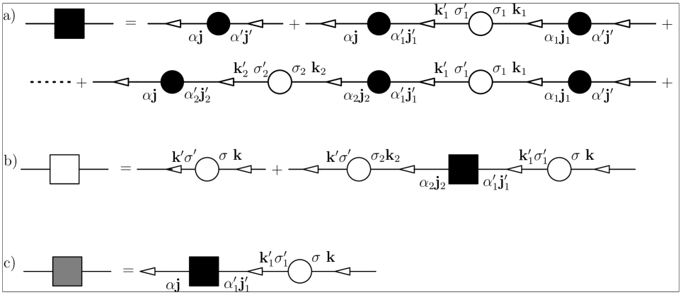
Figure 1: Cumulant expansion diagrams of the PAM, that give the one-electron GF in the Chain Approximation (CHA) Figueira et al. (1994). The filled circles (vertices) corresponds to the $f$-electron cumulants and the empty ones to those of the $c$-electrons. The lines (edges) joining two vertices represent the perturbation (hybridization) (cf. Rules 3.1 and 3.2 in reference Figueira et al. (1994)). a) Diagrams for the $f$-electron GF $G_{j,\alpha;j^{\prime},\alpha^{\prime}}^{ff}(i\omega_{n}=z_{n})$ in the CHA, represented by the filled square to the left. b) Diagrams for the $c$ electron GF $G_{\mathbf{k}^{\mathbf{\prime}}\mathbf{,}\sigma^{\prime};\mathbf{k,}\sigma}^{cc}(z_{n})$ in the CHA, represented by the square symbol to the left. c) Diagrams for the $f$-$c$ electron GF $G_{\mathbf{j};\mathbf{k,}\sigma}^{fc}(z_{n})$ in the CHA, represented by the square symbol to the left.

IV.0.2 The exact formal Green’s functions for the impurity Anderson model

In the impurity case, only the Fourier transform of the imaginary time is necessary (cf. Eq. (38)), and to abbreviate $\left\langle\left(Y\left(f;\mathbf{j,}\alpha,u=-,\omega\right)\ \ Y\left(f;\mathbf{j}^{\prime}\mathbf{,}\alpha^{\prime},u^{\prime},\omega^{\prime}\right)\right)_{+}\right\rangle=\mathcal{G}^{ff}(\mathbf{j},\alpha,u=-,\omega;\mathbf{j}^{\prime},\alpha^{\prime},u^{\prime},\omega^{\prime})$ we define $\mathcal{G}_{\alpha\alpha^{\prime}}^{ff}(\mathbf{j},i\omega)$. Instead of Eq. (39) we then have:

$$\mathcal{G}^{ff}(\mathbf{j},\alpha,u=-,\omega;\mathbf{j}^{\prime},\alpha^{\prime},u^{\prime},\omega^{\prime})=\mathcal{G}_{\alpha\alpha^{\prime}}^{ff}(\mathbf{j},i\omega)\ \Delta\left(u+u^{\prime}\right)\ \Delta\left(\omega+\omega^{\prime}\right)\ \delta\left(\mathbf{j,j}^{\prime}\right),$$ (52)

and most of the derivation employed in the previous section can be extended to this case.

The contribution to $\mathcal{G}_{\alpha\alpha^{\prime}}^{ff}(\mathbf{j}_{i},z)$ of the term in the series that has $n+1$ effective cumulants is given again by (cf. Eq. (173) in Appendix D)

$$\left\{\left(\mathbf{M\cdot W}\right)^{n}\cdot\mathbf{M}\right\}_{\alpha\alpha^{\prime}}=\left\{\mathbf{M\cdot}\left(\mathbf{W\cdot M}\right)^{n}\right\}_{\alpha\alpha^{\prime}},$$

where $\mathbf{M}$ is defined in Eq. (171):

$$\left\{\mathbf{M}\right\}_{{}_{\alpha,\alpha^{\prime}}}=M_{\alpha\alpha^{\prime}}^{eff}(\mathbf{j}_{i},z_{n},u),$$ (53)

and $\mathbf{W}$ in Eqs. (172,169)

$$\left\{\mathbf{W}\right\}_{{}_{\alpha^{\prime},\alpha}}=W_{\alpha^{\prime},\alpha}\left(\sigma,z_{n}\right)=\frac{1}{N_{s}}\sum_{\mathbf{k}}V^{\ast}(\alpha^{\prime},\mathbf{k},\sigma)V(\alpha,\mathbf{k},\sigma)\ \mathcal{G}_{c,\sigma}^{0}\left(\mathbf{k},z_{n}\right).$$ (54)

As before we define a matrix

$$\mathbf{A=W\cdot M}$$ (55)

with components

$$A_{\alpha\alpha^{\prime}}\left(\mathbf{k},\sigma,z_{n}\right)\equiv\left(\mathbf{W\cdot M}\right)_{\alpha\alpha^{\prime}},$$ (56)

and then we obtain a matrix with components $\mathcal{G}_{\alpha\alpha^{\prime}}^{ff}(\mathbf{j}_{i},z_{n})$:

$$\mathbf{G}^{ff}=\mathbf{M\cdot}\left(\mathbf{I-A}\right)^{-1}.$$ (57)

As before

$$\mathbf{M=}\left(\mathbf{I+G}^{ff}\cdot\mathbf{W}\right)^{-1}\cdot\mathbf{G}^{ff}.$$ (58)

and if we substitute $\mathbf{G}^{ff}\left(\mathbf{j}_{i},z_{n}\right)$ by $\mathbf{G}^{ff,at}(\mathbf{j}_{i},z_{n})=\mathbf{G}^{ff,at}\left(z_{n}\right)$ we obtain an approximate effective cumulant for the impurity problem.

$$\mathbf{M}^{ap}\left(z_{n}\right)\mathbf{=}\left(\mathbf{I+G}^{ff,at}\left(z_{n}\right)\cdot\mathbf{W}\right)^{-1}\cdot\mathbf{G}^{ff,at}\left(z_{n}\right)$$ (59)

Introducing $\mathbf{M}^{ap}\left(z_{n}\right)$ into Eqs. (55,57) we obtain the approximate GF we shall use in our calculations.

V Calculation of the atomic Green’s functions

When the conduction band has zero width and the hybridization is local (i.e. independent of k), the eigenvalue problem of the Hamiltonian introduced in Eqs. (7,8) has an exact solution Foglio and Falicov (1979), and the GFs can be calculated analytically. Taking $E_{\mathbf{k},\sigma}=E_{0}^{a}$ and $V_{j\alpha,\mathbf{k},\sigma}=V_{j\alpha,\sigma}$ the problem becomes fully local, and one can use the Wannier representation for the creation and annihilation operators $C_{j\mathbf{,}\sigma}^{\dagger}$ and $C_{j,\sigma}$ of the c-electrons. We then write $H_{r}=\sum_{j}H_{j}$, where $H_{j}$ is the local Hamiltonian

$$H_{j}=\sum_{\sigma}\ \left\{E_{0}^{a}\ C_{j\mathbf{,}\sigma}^{\dagger}C_{j,\sigma}+\ \sum_{a}E_{ja}X_{j,aa}+\sum_{\alpha,\sigma}\left(V_{j\alpha,\sigma}X_{j,\alpha}^{\dagger}C_{j\sigma}+V_{j\alpha,\sigma}^{\ast}C_{j\sigma}^{\dagger}X_{j,\alpha}\right)\right\},$$ (60)

and the subindex $j$ can be dropped because we assume a uniform system.

We shall denote with $\left|n,r\right\rangle$ the eigenstates of the Hamiltonian $H_{j}$ with eigenvalues $E_{n,r},$ where $n$ is the total number of electrons in that state, and $r$ characterizes the different states. These eigenstates satisfy

$$\mathcal{H}\ \left|n,r\right\rangle=\varepsilon_{n,r}\ \left|n,r\right\rangle,$$ (61)

where $\mathcal{H}$ corresponds to that in Eq. (11) but for a single site, and $\varepsilon_{n,r}=E_{n,r}-n\mu$ (cf. Eq. (12)). The states $\left|n,r\right\rangle$ are usually obtained by diagonalization, and employing Eqs. (15,61) we find

$$\exp\left[-\beta\mathcal{H}\right]\hat{Y}(\gamma,\tau)\hat{Y}(\gamma^{\prime},0)\left|n,r\right\rangle =\sum_{n^{\prime}n^{\prime\prime}r^{\prime}r^{\prime\prime}}\exp\left[\mathcal{H}\left(\tau-\beta\right)\right]\ \left|n^{\prime\prime},r^{\prime\prime}\right\rangle\left\langle n^{\prime\prime},r^{\prime\prime}\right|\ Y_{\gamma}\exp\left[-\mathcal{H}\tau\right]\left|n^{\prime},r^{\prime}\right\rangle\left\langle n^{\prime},r^{\prime}\right|\ Y_{\gamma^{\prime}}\ \left|n,r\right\rangle$$

$$=\sum_{n^{\prime}n^{\prime\prime}r^{\prime}r^{\prime\prime}}\exp\left[-\beta\varepsilon_{n^{\prime\prime},r^{\prime\prime}}+\left(\varepsilon_{n^{\prime\prime},r^{\prime\prime}}-\varepsilon_{n^{\prime},r^{\prime}}\right)\tau\right]\left\langle n^{\prime\prime},r^{\prime\prime}\right|\ Y_{\gamma}\left|n^{\prime},r^{\prime}\right\rangle\left\langle n^{\prime},r^{\prime}\right|\ Y_{\gamma^{\prime}}\ \left|n,r\right\rangle\ \left|n^{\prime\prime},r^{\prime\prime}\right\rangle$$ (62)

Employing Eq.(119) of Appendix (C) we calculate the Fourier transform of $\left\langle\left(X_{j,\alpha}(\tau)X_{j,\alpha^{\prime}}^{\dagger}(\tau^{\prime})\right)_{+}\right\rangle_{\mathcal{H}}$:

$$\left\langle\left(X_{j,\alpha}(\omega_{s})\ X_{j,\alpha^{\prime}}^{\dagger}(\omega_{s}^{\prime})\right)_{+}\right\rangle_{\mathcal{H}}=\ \Delta\left(\omega_{s}+\omega_{s}^{\prime}\right)\int_{0}^{\beta}d\tau\ \left\langle\left(X_{j,\alpha}(\tau)X_{j,\alpha^{\prime}}^{\dagger}(0)\right)_{+}\right\rangle_{\mathcal{H}}\exp\left[i\tau\ \omega_{s}\right]$$ (63)

and we shall then abbreviate

$$\left\langle\left(X_{j,\alpha}(\omega_{s})\ X_{j,\alpha^{\prime}}^{\dagger}(\omega_{s}^{\prime})\right)_{+}\right\rangle_{\mathcal{H}}=\Delta(\omega_{s}+\omega_{s}^{\prime})\ \mathcal{G}_{\alpha\alpha^{\prime}}^{ff,at}(i\omega_{s}).$$ (64)

Employing the grand canonical potential $\Omega=-kT\ln\sum\exp(-\beta\epsilon_{n,r})$ Martinez (1989) we find for $0\leq\tau\leq\beta$

$$\left\langle\left(X_{j,\alpha}(\tau)X_{j,\alpha^{\prime}}^{\dagger}(0)\right)_{+}\right\rangle_{\mathcal{H}}=\exp\left(\beta\Omega\right)\ \left\{\sum_{n,r}\left\langle n,r\right|\exp\left[-\beta\mathcal{H}\right]\ X_{j,\alpha}(\tau)\ X_{j,\alpha^{\prime}}^{\dagger}(0)\ \left|n,r\right\rangle\right\},$$ (65)

and from Eq. (62)

$$\left\langle\left(X_{j,\alpha}(\tau)X_{j,\alpha^{\prime}}^{\dagger}(0)\right)_{+}\right\rangle_{\mathcal{H}}=\exp\left(\beta\Omega\right)\ \left\{\sum_{n,r,n^{\prime},r^{\prime}}\exp\left[-\beta\varepsilon_{n,r}+\left(\varepsilon_{n,r}-\varepsilon_{n^{\prime},r^{\prime}}\right)\tau\right]\ \left\langle n,\sigma r\right|\ X_{j,\alpha}\left|n^{\prime},r^{\prime}\right\rangle\left\langle n^{\prime},r^{\prime}\right|\ X_{j,\alpha^{\prime}}^{\dagger}\ \left|n,r\right\rangle\right\}.$$ (66)

Integrating Eq. (66) and using $\exp\left[i\ \omega_{s}\beta\right]=-1$ and the properties of the $X_{j,\alpha}$ we obtain from Eqs. (63-64)

$$\mathcal{G}_{\alpha\alpha^{\prime}}^{ff,at}(i\omega_{s})=-e^{\beta\Omega}\sum_{n,r,r^{\prime}}\frac{\exp(-\beta\varepsilon_{n-1,r})+\exp(-\beta\varepsilon_{n,r^{\prime}})}{i\omega_{s}+\varepsilon_{n-1,r}-\varepsilon_{n,r^{\prime}}}\left\langle n-1,r\right|\ X_{j,\alpha}\left|n,r^{\prime}\right\rangle\left\langle n,r^{\prime}\right|\ X_{j,\alpha^{\prime}}^{\dagger}\ \left|n-1,r\right\rangle.$$ (67)

Equivalent expressions for $\mathcal{G}_{\sigma\sigma^{\prime}}^{cc,at}(i\omega_{s}),\mathcal{G}_{\alpha\sigma^{\prime}}^{fc,at}(i\omega_{s}),\mathcal{G}_{\sigma\alpha^{\prime}}^{cf,at}(i\omega_{s})$ are easily obtained. One can also consider these functions as matrix elements of four matrices $\mathbf{G}^{ff,at}(i\omega_{s})$, $\mathbf{G}^{cc,at}(i\omega_{s})$, $\mathbf{G}^{fc,at}(i\omega_{s})$ and $\mathbf{G}^{cf,at}(i\omega_{s})$, and one can also define a larger matrix $\mathbf{G}^{at}(i\omega_{s})$ that includes these four matrices, but it is not yet clear whether a formulation that uses this larger matrix would have any advantage. We then define

$$\mathbf{G}^{at}(i\omega_{s})=\begin{bmatrix}\mathbf{G}^{ff,at}(i\omega_{s})&\mathbf{G}^{fc,at}(i\omega_{s})\\ \mathbf{G}^{cf,at}(i\omega_{s})&\mathbf{G}^{cc,at}(i\omega_{s})\end{bmatrix},$$ (68)

which would be a $6\times 6$ matrix for finite $U$ and a $4\times 4$ matrix for infinite $U$.

VI Detailed calculation of the approximate GF

VI.1 Introduction

The hybridization constant $V_{j,\mathbf{k},\sigma}$ in Eq. (2) is given by Eq. (3),

$$V_{j,\mathbf{k},\sigma}=\frac{1}{\sqrt{N_{s}}}V_{\sigma}(\mathbf{k})\exp{(i\mathbf{k}.\mathbf{R}_{j}),}$$

and when the Hubbard operators are introduced into Eq. (2) , the hybridization Hamiltonian $H_{h}$ is transformed into Eq. (8):

$$H_{h}=\sum_{jba,\vec{k}\sigma}\left(V_{jba,\mathbf{k}\sigma}X_{j,ba}^{\dagger}C_{\mathbf{k}\sigma}+V_{jba,\mathbf{k}\sigma}^{\ast}C_{\mathbf{k}\sigma}^{\dagger}X_{j,ba}\right),$$

with hybridization constant $V_{j\alpha,\mathbf{k}\sigma}$. The $\alpha=(b,a)$ describes the transition $\mid a>\rightarrow\mid b>$, where the local state $\mid a>$ has one electron more than the state $\mid b>$. To simplify the calculation one defines the parameters $v(j,\alpha,\mathbf{k},\sigma,u)$ in Eq. (16)

$$\begin{array}[]{ccc}v(j,\alpha,\mathbf{k},\sigma,+)&=&V_{j,ba,\mathbf{k},\sigma},\\ v(j,\alpha,\mathbf{k},\sigma,-)&=&V_{j,ba,\mathbf{k},\sigma}^{\ast},\end{array}$$

where $u=\pm$, and in the PAM we use $V(\alpha,\mathbf{k},\sigma,u)$, defined in Eq. (27)

$$v(j,\alpha,\mathbf{k},\sigma,u)=V(\alpha,\mathbf{k},\sigma,u)N_{s}^{-\frac{1}{2}}\exp(iu\mathbf{k}.\mathbf{R}_{j}).$$

After applying the rules for calculating the GF, it is convenient to return to the explicit use of complex conjugates, and we introduce $V(\alpha,\mathbf{k},\sigma)$ in Eq. (135)

$$V(\alpha,\mathbf{k},\sigma)\equiv V(\alpha,\mathbf{k},\sigma,u=-),$$ (69)

so that Eq. (136)

$$V^{\ast}(\alpha,\mathbf{k},\sigma)\equiv V(\alpha,\mathbf{k},\sigma,u=+)$$ (70)

follows from Eq. (27).

There are four local states $\mid 0>$, $\mid+>$, $\mid->$ and $\mid d>=\mid+,->$ per site, and there are only four $X$ operators that destroy one local electron at a given site. We use the index $I_{x}=1,2,3,4$ to characterize these $X$ operators:

$$I_{x}$$

(71)

so that $I_{x}=1,3$ destroy one electron with spin up and $I_{x}=2,4$ destroy one electron with spin down. We use $\sigma=+$ and $\sigma=-$ instead of $\sigma=\uparrow$ and $\sigma=\downarrow$ to emphasize that the spin belongs to a local electron.

The matrix $\mathbf{W}$, employed in the PAM calculation, is defined in Eq. (148)

$$\left\{\mathbf{W}\right\}_{{}_{\alpha^{\prime},\alpha}}=W_{\alpha^{\prime},\alpha}\left(\mathbf{k},\sigma,z_{n}\right),$$

and its matrix elements are defined in Eq. (145)

$$W_{\alpha^{\prime},\alpha}\left(\mathbf{k},\sigma,z_{n}\right)=V^{\ast}(\alpha^{\prime},\mathbf{k},\sigma)V(\alpha,\mathbf{k},\sigma)\ \mathcal{G}_{c,\sigma}^{0}\left(\mathbf{k},z_{n}\right),$$

where  $z_{n}=i\omega_{n}$ are the Matsubara frequencies. A related matrix appears in the impurity case in Eq. (172)

$$\left\{\mathbf{W}\right\}_{{}_{\alpha^{\prime},\alpha}}=W_{\alpha^{\prime},\alpha}\left(\sigma,z_{n}\right).$$

with matrix elements defined in Eq. (169)

$$W_{\alpha^{\prime},\alpha}\left(\sigma,z_{n}\right)=\frac{1}{N_{s}}\sum_{\mathbf{k}}V^{\ast}(\alpha^{\prime},\mathbf{k},\sigma)V(\alpha,\mathbf{k},\sigma)\ \mathcal{G}_{c,\sigma}^{0}\left(\mathbf{k},z_{n}\right).$$

The hybridization is spin independent in the Anderson model, so we have

$$V(0\sigma,\mathbf{k},\bar{\sigma})=V(\bar{\sigma}d,\mathbf{k},\bar{\sigma})=V(0\bar{\sigma},\mathbf{k},\sigma)=V(\sigma d,\mathbf{k},\sigma)=0.$$

We shall assume a purely local mixing, so that $V_{\sigma}(\mathbf{k})$ in Eq. (8)  is $\mathbf{k}$ independent, and when we introduce the Hubbard operators we obtain

$$V(0\sigma,\mathbf{k},\sigma) =V,$$ (72)

$$V(\bar{\sigma}d,\mathbf{k},\sigma) =\sigma V,$$ (73)

where we have also assumed that $V_{\sigma}(\mathbf{k})$ is independent of $\sigma=\pm 1$.

As discussed in the introduction of Section III,when the Hamiltonian is spin independent or commutes with the $z$ component of the spin, the $4\times 4$ matrices $\mathbf{G}^{ff}$, $\mathbf{M}$,  $\mathbf{W}$ and $\mathbf{A=W.M}$ can be diagonalized into two $2\times 2$ matrices, e.g.:

$$\mathbf{G}^{ff}=\begin{pmatrix}\mathbf{G}_{\uparrow}^{ff}&0\\ 0&\mathbf{G}_{\downarrow}^{ff}\end{pmatrix}.$$ (74)

In this matrix the indices $I_{x}$ defined in Eq. (71) have been rearranged, so that $I_{x}=1,3$ appear in $\mathbf{G}_{\uparrow}^{ff}$ and $I_{x}=2,4$ appear in $\mathbf{G}_{\downarrow}^{ff}$.

Employing Eqs. (72,73) we find for the PAM (cf. Eq. (42))

$$\mathbf{W}_{\uparrow}\left(\mathbf{k},z\right) =\ \left|V\right|^{2}\ \mathcal{G}_{c,\uparrow}^{0}\left(\mathbf{k},z\right)\ \begin{pmatrix}1&1\\ 1&1\end{pmatrix},$$ (75)

$$\mathbf{W}_{\downarrow}\left(\mathbf{k},z\right) =\ \left|V\right|^{2}\ \mathcal{G}_{c,\downarrow}^{0}\left(\mathbf{k},z\right)\ \begin{pmatrix}1&-1\\ -1&1\end{pmatrix}.$$ (76)

For an impurity located at the origin we find

$$\mathbf{W}_{\uparrow}\left(z\right) =\left|V\right|^{2}\varphi_{\uparrow}(z)\begin{pmatrix}1&1\\ 1&1\end{pmatrix},$$ (77)

$$\mathbf{W}_{\downarrow}\left(z\right) =\left|V\right|^{2}\varphi_{\downarrow}(z)\ \begin{pmatrix}1&-1\\ -1&1\end{pmatrix},$$ (78)

where

$$\varphi_{\sigma}(z)=\frac{1}{N_{s}}\sum_{\mathbf{k}}\ \mathcal{G}_{c,\sigma}^{0}\left(\mathbf{k},z\right).$$ (79)

For a rectangular band with half-width $D$ in the interval $[A,B],$ with $B=A+2D$ we find (the minus sign of $\mathcal{G}_{c,\sigma}^{0}\left(\mathbf{k},z\right)$ is included in the logarithm)

$$\varphi_{\sigma}(z)=\frac{1}{2D}\ \ln\frac{z-B+\mu}{z+A+\mu},$$ (80)

where the $\mu$ appears in $\varphi_{\sigma}(z)$ because of the $\varepsilon\left(\mathbf{k},\sigma\right)=E_{\mathbf{k,\sigma}}-\mu$ in $\mathcal{G}_{c,\sigma}^{0}\left(\mathbf{k},z\right)$ .

Both for the PAM (Eq. (47)) and for the SIAM (Eq. (57)) we have the same relation for the submatrices in Eq. (74):

$$\mathbf{G}_{\sigma}^{ff}=\mathbf{M}_{\sigma}\mathbf{\cdot}\left(\mathbf{I-A}_{\sigma}\right)^{-1},$$ (81)

and as before (cf. Section III)

$$\mathbf{M}_{\sigma}\mathbf{=}\left(\mathbf{I+G}_{\sigma}^{ff}\cdot\mathbf{W}_{\sigma}\right)^{-1}\cdot\mathbf{G}_{\sigma}^{ff}.$$ (82)

VI.2 The approximate $\mathbf{G}_{\sigma}^{ff,ap}$ GF for the Periodic Anderson Model

The calculation of the exact effective cumulants $\mathbf{M}_{\sigma}$ is as difficult as that of the exact $\mathbf{G}_{\sigma}^{ff}$, and the atomic approach consists in using instead the $\mathbf{M}_{\sigma}$ of a similar model that is exactly soluble. Taking a conduction band of zero width at $\varepsilon_{o}=E_{0}-\mu$ and a local hybridization, the PAM becomes a collection of independent atomic Anderson systems that can be solved exactly, and we call this solution the atomic Anderson solution (AAS). We then employ the AAS to calculate the corresponding exact Green’s function $\mathbf{G}_{\sigma}^{ff,at}(z)$, and we define an approximate effective cumulant $\mathbf{M}_{\sigma}^{ap}$ by introducing this GF into Eq.(82) using $\mathcal{G}_{c,\sigma}^{0,at}\left(i\omega\right)=-1/\left(i\omega-\varepsilon_{0}\right)$ in the corresponding $\mathbf{W}^{at}$. This procedure overestimates the contribution of the $c$ electrons  Alascio et al. (1979)Alascio et al. (1980), because we concentrate them at a single energy level $E_{o}$, and to moderate this effect we replace $V^{2}$ by $\Delta^{2}$ in the calculation of the $\mathbf{M}_{\sigma}^{ap}$, where $\Delta=\pi\left|V\right|^{2}/2D$ is the Anderson parameter (but we keep the full $\left|V\right|^{2}$ when we substitute this $\mathbf{M}_{\sigma}^{ap}$ into Eq. (81) to calculate the approximate $\mathbf{G}_{\sigma}^{ff,ap}$).

VI.2.1 Imaginary frequency and reciprocal space

To calculate the approximate $\mathbf{G}_{\sigma}^{ff,ap}(\mathbf{k},i\omega)$ for imaginary frequency and reciprocal space we then introduce the $\mathbf{M}_{\sigma}^{ap}$ into Eq. (81), with $\mathbf{A}_{\sigma}^{ap}\mathbf{=W}_{\sigma}\mathbf{.M}_{\sigma}^{ap}$ and $\mathbf{W}_{\sigma}$ defined in Eqs. (75,76) with the full $\left|V\right|^{2}$. We can now write

$$\mathbf{M}_{\uparrow}^{ap}=\begin{pmatrix}m_{11}&m_{13}\\ m_{31}&{}_{m33}\end{pmatrix}\hskip 20.0pt\mathrm{;\hskip 20.0pt}\mathbf{M}_{\downarrow}^{ap}=\begin{pmatrix}m_{22}&m_{24}\\ m_{42}&{}_{m44}\end{pmatrix},$$ (83)

and

$$\mathbf{A}_{\uparrow}^{ap}=\begin{pmatrix}a_{11}&a_{13}\\ a_{31}&a_{33}\end{pmatrix}\hskip 20.0pt\mathrm{;\hskip 20.0pt}\mathbf{A}_{\downarrow}^{ap}=\begin{pmatrix}a_{22}&a_{24}\\ a_{42}&a_{33}\end{pmatrix},$$ (84)

and from Eqs. (75,76) we find

$$a_{11}=\mathcal{G}_{c,\uparrow}^{0}\left(\mathbf{k},z\right)\left(m_{11}+m_{31}\right)$$      ;

     ;

     ;

     ;

                       (85)

To derive our approximate $\mathbf{G}_{\sigma}^{ff,ap}$ we substitute both $\mathbf{M}_{\sigma}^{ap}$ and $\mathbf{A}_{\sigma}^{ap}\mathbf{=W}_{\sigma}\mathbf{.M}_{\sigma}^{ap}$ into Eq. (81), and we obtain

$$\mathbf{G}_{\uparrow}^{ff,ap}(\mathbf{k},i\omega)=\frac{\begin{pmatrix}m_{11}&m_{13}\\ m_{31}&{}_{m33}\end{pmatrix}-\left|V\right|^{2}\mathcal{G}_{c,\uparrow}^{0}\left(\mathbf{k},z\right)\left(m_{11}m_{33}-m_{13}m_{31}\right)\begin{pmatrix}1&-1\\ -1&1\end{pmatrix}}{1-\left|V\right|^{2}\mathcal{G}_{c,\uparrow}^{0}\left(\mathbf{k},z\right)\left(m_{11}+m_{33}+m_{13}+m_{31}\right)},$$ (86)

and

$$\mathbf{G}_{\downarrow}^{ff,ap}(\mathbf{k},i\omega)=\frac{\begin{pmatrix}m_{22}&m_{24}\\ m_{42}&{}_{m44}\end{pmatrix}-\left|V\right|^{2}\mathcal{G}_{c,\downarrow}^{0}\left(\mathbf{k},z\right)\left(m_{22}m_{44}-m_{24}m_{42}\right)\begin{pmatrix}1&1\\ 1&1\end{pmatrix}}{1-\left|V\right|^{2}\mathcal{G}_{c,\downarrow}^{0}\left(\mathbf{k},z\right)\left(m_{22}+m_{44}-m_{24}-m_{42}\right)}.$$ (87)

Note that in this approach the $\mathbf{M}_{\sigma}^{ap}(i\omega)$ are independent of $\mathbf{k},$ and that all the $\mathbf{k}$ dependence of our approximate $\mathbf{G}_{\sigma}^{ff,ap}(\mathbf{k},i\omega)$ comes through the $\mathcal{G}_{c,\sigma}^{0}\left(\mathbf{k},i\omega\right)$ in the Eqs. (86-87)

VI.2.2 Real space and imaginary frequency

In the previous section we derived the reciprocal space and imaginary frequency GF for the PAM in the atomic approximation, but sometimes it is necessary to use the GF in real space, with the $f$ electron being created and destroyed at the same site. These GF are denoted by $G_{\sigma}^{ff}(i\omega)$ and are given by

$$\mathbf{G}_{\sigma}^{ff}(i\omega)=\frac{1}{N}\sum_{\mathbf{k}}\mathbf{G}_{\sigma}^{ff}(\mathbf{k},i\omega)=\frac{1}{N}\sum_{\mathbf{k}}\mathbf{G}_{\sigma}^{ff}\left(\varepsilon\left(\mathbf{k}\right),i\omega\right).$$ (88)

Considering a rectangular conduction band and transforming the sum into an integral, we obtain

$$\mathbf{G}_{\sigma}^{ff}(i\omega)=\frac{1}{2D}\int_{-D-\mu}^{+D-\mu}d\varepsilon\mathbf{G}_{\sigma}^{ff}(\varepsilon,i\omega),$$ (89)

where $\mu$ is the chemical potential and $D$ is the half-width of the conduction band. Substituting Eqs. (86 and 87) into Eq. (89) we obtain that

$$\mathbf{G}_{\uparrow}^{ff}(i\omega)=\begin{pmatrix}G_{11}^{ff}&G_{13}^{ff}\\ G_{31}^{ff}&G_{33}^{ff}\end{pmatrix}=\frac{1}{2D}\int_{-D-\mu}^{+D-\mu}d\varepsilon\frac{\mathbf{M}_{\uparrow}^{ap}-\left|V\right|^{2}\mathcal{G}_{c,\uparrow}^{0}(\varepsilon,i\omega)\left(m_{11}m_{33}-m_{13}m_{31}\right)\begin{pmatrix}1&-1\\ -1&1\end{pmatrix}}{1-\left|V\right|^{2}\mathcal{G}_{c,\uparrow}^{0}(\varepsilon,i\omega)\left(m_{11}+m_{33}+m_{13}+m_{31}\right)},$$ (90)

and

$$\mathbf{G}_{\downarrow}^{ff}(i\omega)=\begin{pmatrix}G_{22}^{ff}&G_{24}^{ff}\\ G_{42}^{ff}&G_{44}^{ff}\end{pmatrix}=\frac{1}{2D}\int_{-D-\mu}^{+D-\mu}d\varepsilon\frac{\mathbf{M}_{\downarrow}^{ap}-\left|V\right|^{2}\mathcal{G}_{c,\downarrow}^{0}(\varepsilon,i\omega)\left(m_{22}m_{44}-m_{24}m_{42}\right)\begin{pmatrix}1&1\\ 1&1\end{pmatrix}}{1-\left|V\right|^{2}\mathcal{G}_{c,\downarrow}^{0}(\varepsilon,i\omega)\left(m_{22}+m_{44}-m_{24}-m_{42}\right)}.$$ (91)

The variable $\varepsilon$ is present only in $\mathcal{G}_{c,\sigma}^{0}$ and the integration is straightforward. We find

$$\mathbf{G}_{\uparrow}^{ff}(z)=\mathbf{M}_{\uparrow}^{ap}+\frac{V^{2}}{2D}ln\left(\frac{z-D+\mu+V^{2}M_{\uparrow}^{ff}}{z+D+\mu+V^{2}M_{\uparrow}^{ff}}\right)\left[\mathbf{M}_{\uparrow}^{ap}M_{\uparrow}^{ff}-\begin{pmatrix}1&-1\\ -1&1\end{pmatrix}\Theta_{\uparrow}\right]$$ (92)

$$\mathbf{G}_{\downarrow}^{ff}(z)=\mathbf{M}_{\downarrow}^{ap}+\frac{V^{2}}{2D}ln\left(\frac{z-D+\mu+V^{2}M_{\downarrow}^{ff}}{z+D+\mu+V^{2}M_{\downarrow}^{ff}}\right)\left[\mathbf{M}_{\downarrow}^{ap}M_{\downarrow}^{ff}-\begin{pmatrix}1&1\\ 1&1\end{pmatrix}\Theta_{\downarrow}\right]$$ (93)

where

$$M_{\uparrow}^{ff}=m_{11}+m_{13}+m_{31}+m_{33},$$ (94)

$$M_{\downarrow}^{ff}=m_{22}+m_{44}-m_{24}-m_{42},$$ (95)

and

$$\Theta_{\uparrow}=m_{11}m_{33}-m_{13}m_{31,}$$ (96)

$$\Theta_{\downarrow}=m_{22}m_{33}-m_{24}m_{42}.$$ (97)

In Appendix E we define and calculate the formal expressions of the matrices $\mathbf{G}_{\sigma}^{fc,ap}(\mathbf{k},i\omega)$ (cf. Eq. (178,179)) and $\mathbf{G}_{\sigma}^{cf,ap}(\mathbf{k},i\omega)$ (cf. Eq. (184,185)) associated to the crossed  GF of the impurity, as well as the GF of the pure conduction electron $\mathbf{G}_{\sigma}^{cc,ap}(\mathbf{k},i\omega)$ (cf. Eq. (189,190)). We can also describe the conduction electrons in real space and imaginary time: the corresponding $\mathbf{G}_{\sigma}^{fc,ap}(i\omega)$ are given in Eqs. (191,193) and the $\mathbf{G}_{\sigma}^{cf,ap}(i\omega)$ in Eqs. (194,195). In a similar way we obtain $\mathbf{G}_{\sigma}^{cc,ap}(i\omega)$ (cf. Eq. (196)), and we can use this relation to express all the other GF (cf. Eqs. (197-200,201,202)).

VI.3 The approximate $\mathbf{G}_{\sigma}^{ff,ap}$ GF for the Impurity Anderson Model

As in the case of the PAM, we substitute the $\mathbf{G}_{\sigma}^{ff}$ in Eq. (82) by the exact solution $\mathbf{G}_{\sigma}^{ff,at}$ of the problem with zero band width and local hybridization, and obtain the corresponding effective cumulant $\mathbf{M}_{\sigma}^{ap}$. The conduction band corresponding to this approximation then has $E_{\mathbf{k},\sigma}=E_{0}^{a}$, so that for all values of $\mathbf{k}$ it is $\mathcal{G}_{c,\sigma}^{0}\left(\mathbf{k},z\right)=-1/\left(z-\varepsilon_{o}\right)$ , where $\varepsilon_{o}=E_{0}^{a}-\mu$. From Eq. (79) we then find $\varphi_{\sigma}(z)\rightarrow\varphi_{\sigma}^{0}(z)=-1/\left(z-\varepsilon_{o}\right)$, and substituting into Eqs. (77,78) we obtain the $\mathbf{W}_{\sigma}^{ap}$ that should be used in Eq. (82) to calculate $\mathbf{M}_{\sigma}^{ap}$. To define the approximate GF $\mathbf{G}_{\sigma}^{ff,ap}(i\omega)$ introduced in the present work, we substitute this approximate $\mathbf{M}_{\sigma}^{ap}$ into the exact expression Eq. (81), but in this equation we use the $\mathbf{W}_{\sigma}$ that corresponds to the conduction band with full width. The Eqs. (83,84) for $\mathbf{M}_{\sigma}^{ap}$ and $\mathbf{A}_{\sigma}^{ap}\mathbf{=W}_{\sigma}\mathbf{.M}_{\sigma}^{ap}$ are also valid for the SIAM, but using Eqs. (77,78) we find different expression for the $a_{ij}$:

$$a_{11}=\varphi_{\uparrow}(z)\left(m_{11}+m_{31}\right)$$      ;

     ;

     ;

     ;

                       (98)

If we now substitute these $\mathbf{M}_{\sigma}^{ap}$ and $\mathbf{A}_{\sigma}^{ap}$ into Eq. (81), we obtain the approximate $\mathbf{G}_{\sigma}^{ff,ap}$ for the SIAM:

$$\mathbf{G}_{\uparrow}^{ff,ap}(i\omega)=\frac{\begin{pmatrix}m_{11}&m_{13}\\ m_{31}&{}_{m33}\end{pmatrix}-\left|V\right|^{2}\varphi_{\uparrow}((i\omega))\left(m_{11}m_{33}-m_{13}m_{31}\right)\begin{pmatrix}1&-1\\ -1&1\end{pmatrix}}{1-\left|V\right|^{2}\varphi_{\uparrow}((i\omega))\left(m_{11}+m_{33}+m_{13}+m_{31}\right)},$$ (99)

and

$$\mathbf{G}_{\downarrow}^{ff,ap}(i\omega)=\frac{\begin{pmatrix}m_{22}&m_{24}\\ m_{42}&{}_{m44}\end{pmatrix}-\left|V\right|^{2}\varphi_{\downarrow}((i\omega))\left(m_{22}m_{44}-m_{24}m_{42}\right)\begin{pmatrix}1&1\\ 1&1\end{pmatrix}}{1-\left|V\right|^{2}\varphi_{\downarrow}((i\omega))\left(m_{22}+m_{44}-m_{24}-m_{42}\right)}.$$ (100)

In Appendix E we define and calculate the formal expressions of the matrices $\mathbf{G}_{\sigma}^{fc,ap}(\mathbf{j}_{i}=0,\mathbf{k},i\omega)$ (cf. Eqs. (215,216)) and $\mathbf{G}_{\sigma}^{cf,ap}(\mathbf{k},\mathbf{j}^{\prime}=0,i\omega)$ (cf. Eqs. (221,222)) associated to the crossed  GF of the impurity, as well as the GF of the pure conduction electron $\mathbf{G}_{\sigma}^{cc,ap}(\mathbf{k},\mathbf{k}^{\prime},i\omega)$ (cf. Eqs. (226,227)). We can also describe the conduction electrons in the Wannier representation: the corresponding $\mathbf{G}_{\sigma}^{fc,ap}(i\omega)$ are given in Eqs. (LABEL:E5.32,230) and the $\mathbf{G}_{\sigma}^{cf,ap}(i\omega)$ in Eqs. (231,232). In a similar way we obtain $\mathbf{G}_{\sigma}^{cc,ap}(i\omega)$ (cf. Eq. (233)), and we can use this relation to express all the other GF (cf. Eqs. (234-237,240,241)).

Appendix A The sign of the contribution of a graph.

For convenience we summarize here the Appendix C of reference Figueira et al. (1994), where one should have${}^{\text{\ref{myfoot4}}}$ $v(\alpha,\vec{k},\sigma,\pm u)$ instead of $V(\alpha,\vec{k},\sigma,\pm u)$ in the item 2(b) of Rule C.2.

Here we discuss the sign that must be given to the contribution of a given graph, and we are only interested in the case without external fields, i.e. with $\xi=0$, but we shall keep some results for $\xi\neq 0$ that are convenient to understand $\xi=0$. The rules for drawing the graphs that appear in the calculation of the averages $\left\langle\left(Y(l_{1}),\cdots Y(l_{n})\right)_{+}\right\rangle^{\xi}$ are given in Rules 3.3 and 3.4 in Figueira et al. (1994). In item 4 of those rules, the Fermi type lines running to each vertex were paired in an arbitrary way for $\xi=0$, and several open and closed loops were formed in this way, where all the open loops must have two external vertices. A definite sense was arbitrarily assigned to each of the loops, and we call this direction the “sense of the loop”. In the following discussion we consider only Fermi-type operators, because the position of the Bose-type operators does not affect the sign of the contribution, and we shall mean Fermi-type operator when we say “operator” in the remaining of this Appendix. It is now convenient to introduce two concepts that shall be useful in the present computation.

Definition C.1.

A graph is in a “perfect ordering” when the following relations are satisfied:

1.

For all the open loops, $\tau$ increases in all the vertices of the loop in the sense of the loop.

2.

For every closed loop, $\tau$ increases in the sense of the loop for all the vertices but one (it is impossible to satisfy (1) for a closed loop).

3.

All the $\tau$ in a given loop are either smaller or greater than all the $\tau$ in all the other loops of the graph.$\bullet$

There are many ways to choose a perfect ordering of a graph, but the particular choice is not important provided that we use always the same one after it has been chosen.

Definition C.2.

Several Fermi-type operators of a graph contribution are in a “perfect order” when:

1.

The $Y$-operators are written from right to left following the perfect ordering we have chosen for their graph.

2.

For the two operators of each internal edge (they have the same $\tau$) we write the $X$-operator to the left of the $C$-operator.$\bullet$

As a starting point we shall consider rules that are also valid for $\xi\neq 0$ because they are simpler to state although less systematic to apply than those given by Hubbard Hubbard (1966) for $\xi=0$. We shall consider explicitly the graphs for $\left\langle\left(\hat{Y}(1)\cdots\hat{Y}(r)\right)_{+}\right\rangle_{H}$, i.e. a GF with $r$ external operators $\hat{Y}(1)\cdots\hat{Y}(r)$ (but the rules are also valid for vacuum graphs). The $n$-th order term of this GF contains the average

$$\left\langle\left(\hat{Y}(1)\cdots\hat{Y}(r)\left(H^{\prime}(\tau_{1})\cdots H^{\prime}(\tau_{n})\right)\right)_{+}\right\rangle_{H}$$ (101)

and the application of Theorem 3.1 from Figueira et al. (1994) to this equation gives all the $n$-th order graphs.

Rule C.1.

To obtain the sign associated to a given graph, multiply the parities of the following two permutations:

1.

It takes the operators from the order used to write Eq. (101) into the perfect order.

2.

It takes the operators from the perfect order into the order in which they appear in the final expression that gives the graph contribution.

As the operators $H_{h}$ are of the Bose type and can be moved freely inside the ordered parenthesis in Eq. (101), in the first step it is necessary to consider only the permutation that takes the external Fermi-type operators to their perfect order. The Rule C.1. is just the application of Theorem 3.1 in Figueira et al. (1994) in two steps, and the only reason to proceed in this way is that the perfect order of the $Y$-operators in a graph provides a reference frame to organize the calculation.

For $\xi=0$ we shall give rules with the same labels employed by Hubbard Hubbard (1966), because of their similarity. In this case, there is only an even number of lines running into each vertex, and for any CV this number is two .This simplifies the treatment, and the first step is the same step 1) employed in Rule C.1: this is just rule “d” of Hubbard.

To calculate the change of sign that corresponds to step 2) in Rule C.1 we proceed in three steps.

First we consider all the open loops that pass through each vertex, and note that in the perfect order, the $X$-operator is to the left of the $C$-operator in all the internal edges. To be able to pair operators of the same type at each vertex (otherwise the corresponding cumulant vanish) it is necessary to change the order of these two operators (with a change of sign) when the arrow in the edge points towards the CV. To correct for the sign missing in Eq. (16) one must also add a factor $\pm u$ to the $v(j,\alpha,\vec{k},\sigma,\pm u)$ in Rule 3.5.2.c in Figueira et al. (1994), and these two factors correspond to Hubbard’s rule “b”. In the present problem there are only two edges at each CV, and when both are internal, the effect cancels out and the rule is not necessary. To prove this result, note that according to Rule 3.6b^′ in Figueira et al. (1994), the cumulant

$$\left\langle\left(Y(c;\vec{k}_{s},\sigma_{2},-u_{2},\tau_{2})Y(c;\vec{k}_{s},\sigma_{1},+u_{1},\tau_{1})\right)_{+}\right\rangle_{c}$$ (102)

at each CV, is already written with the $Y$-operators in the perfect order, with the $-u_{2}$ corresponding to the outgoing arrow. The contribution to Rule 3.5.2.c in Figueira et al. (1994) of the two internal edges running into the CV after correcting for the missing sign in Eq. (16), is then

$$(+u_{2})v(j_{2},\alpha_{2},k_{s},\sigma_{2},+u_{2})(-u_{1})v(j_{1},\alpha_{1},k_{s},\sigma_{1},-u_{1})$$ (103)

As there is particle conservation, we have $u_{1}=u_{2}$, and when we multiply into the minus sign due to the exchange of the X with the C operators on the line with the arrow towards the CV, the overall sign is always plus. Hubbard’ s rule “b” is therefore not necessary for all the CV with two internal lines.

For any CV with only one internal line (and therefore one external line also), one must multiply the $v(j,\alpha,\vec{k},\sigma,\pm u)$ into $\pm u$ and also into $-1$ when the internal edge points toward the CV . This is the only effect that remains in the PAM of Hubbard’s rule “b”.

The discussion above fails for closed loops because $\tau$ can increase in the sense of the loop in all vertices but one. After putting all the operators in perfect order and then exchanging the $X$-operator with the $C$-operator for all the lines with arrows pointing to a CV, the first and last operators in the resulting expression belong to the same vertex, and should therefore be brought together . These two operators are separated by an even number of Fermi operators, but bringing them together by an even permutation would still leave them against the order of the loop, i.e.: the operator at the left would correspond to the edge with the arrow pointing toward the vertex. A permutation of odd parity is then necessary to put all the operators of any closed loop in perfect order, and this is Hubbard’s rule “c”.

After the three steps discussed above, the $Y$-operators that were in the order given by Eq. (101) are now paired at each vertex according to the loops of the graph considered, each pair written in the sense of the loop. We shall denote with $(\alpha_{s},\beta{{}_{s}})$ the two indices of the $Y$-operators of each of those pairs, written already in the sense of the loop,i.e.: $\beta_{s}\rightarrow\alpha_{s}$. All the pairs that correspond to a given vertex are still separated by many pairs that belong to other vertices of the graph, but it is only necessary an even permutation to put together all the pairs of each vertex. The pair associated to each CV is already in the same order of the cumulant of Rule $3.6$ $b^{\prime}$ in Figueira et al. (1994), and only remains to consider the cumulants associated to the FV. If there are $p$ loops crossing an FV, we have already the corresponding operators in the order $(\alpha_{1},\beta_{1}),\cdots(\alpha_{p},\beta_{p})$ while in the cumulant associated to that vertex by Rule 3.6.(2).a in Figueira et al. (1994) they are written in the order $Y(\gamma_{1})\cdots Y(\gamma_{2p})$, where $\gamma_{1}\cdots\gamma_{2p}$, correspond to the same$(\alpha_{1},\beta{1}),\cdots(\alpha_{p},\beta{p})$ but in a different order. It is then necessary to associate to each of these cumulants a $\pm$ given by the parity of the permutation that takes $(\alpha_{1},\beta_{{1}}),\cdots(\alpha_{p},\beta_{{p}})$ into $\gamma_{1}\cdots\gamma_{2p}$. This is Hubbard’s rule “a”.

It is now convenient to put together the rules for the calculation of the sign required by Rule 3.7.(2).d or Rule 3.7a.(2).e.

Rule C.2

To calculate the sign of a graph with $\xi=0$

1.

Define a perfect ordering for the graph according to Definition C.1.

2.

The sign of the graph is the product of the following factors

(a)

When there are $p$ loops crossing an FV, denote with $(\alpha_{s},\beta_{s})$ the indices of the two $X$-operators of the $s$-th loop at that vertex $(s=1,\cdots,p)$, written already in the sense of the loop (i.e.: $\beta_{s}\rightarrow\alpha_{s}$). The $2p$ Fermi-type operators at that FV appear in the cumulant of Rule 3.6a in the order $Y(\gamma_{1})\cdots Y(\gamma_{2p})$, where the $\gamma_{1}\cdots\gamma_{2p}$ are the same $(\alpha_{1},\beta_{1}),\cdots(\alpha_{p},\beta_{p})$ in a different order. For each FV multiply into a $\pm 1$ given by the parity of the permutation that takes$(\alpha_{1},\beta_{1}),\cdots(\alpha_{p},\beta_{p})$ into $\gamma_{1},\cdots\gamma_{2p}$.

(b)

For any CV with only one internal edge multiply the $V(\alpha,\vec{k},\sigma,\pm u)$ of Rule 3.6.(2).c into $(\pm u)$, and also into a further $-1$ when the arrow of the internal edge points toward the CV.

(c)

There is a factor $-1$ for every closed loop.

(d)

If the graph is employed to calculate a GF with $r$ Fermi-type operators written in the order $\hat{Y}(1)\cdots\hat{Y}(r)$, multiply into a sign given by the parity of the permutation that takes $(Y(1)\cdots Y(r))$ into the same operators written in the perfect ordering chosen for the graph. This item does not apply to vacuum graphs.

Appendix B Counting graphs and the symmetry factor.

For convenience we reproduce here, with very minor changes, the Appendix D of reference Figueira et al. (1994).

As discussed in appendix A of reference Figueira et al. (1994), the n-th order term of the perturbative expansion of the GF $\left\langle\left(\hat{Y}(1)\cdots\hat{Y}(r)\right)_{+}\right\rangle_{H}$ contains the expression in Eq. (101) of Figueira et al. (1994), and its contributions have the form

$$\frac{(-1)}{n!}^{n}\mathcal{Z}_{o}(\beta,\xi)\int_{0}^{\beta}d\tau_{1}\sum_{l_{1},l_{1}^{\prime}}V(l_{1},l_{1}^{\prime})\cdots\int_{0}^{\beta}d\tau_{n}$$

$$\sum_{l_{n}\ ,\ l^{\prime}{}_{n}}V(l_{n},l^{\prime}{}_{n})\left\langle\left(Y(l_{1})Y(l_{1}^{\prime})\cdots Y(l_{n})Y(l_{n}^{\prime})\right)_{+}\right\rangle^{\xi}$$ (104)

(cf. Eq. (3.11) in Figueira et al. (1994)), but with the $r$ external operators $Y(1)\cdots Y(r)$ included in the averages. When the Theorem 3.1 in Figueira et al. (1994) is applied to these averages, the $n$-th order contribution can be associated to a family of graphs, and many of them are disconnected and composed of several connected graphs. We label each topologically distinct connected graph with an index $\alpha$, and we use $n_{\alpha}$ to denote the number of times that the $\alpha$ graph appears in the nth-order graph. It is clear that there might be several identical contributions associated to the same $n$-th order graph because all the $n!$ permutations of the edges of a given graph give the same contribution. These identical contributions should be counted as different contributions every time they correspond to a different partition in cumulants. The correct number of times that a topologically distinct graph of $n$-th order gives the same contribution is then

$$n!\prod^{\infty}_{\alpha=1}\frac{1}{n_{\alpha}!g^{n_{\alpha}}_{\alpha}}$$ (105)

where $g_{\alpha}$ is the symmetry factor of the connected graph $\alpha$ and is calculated using the Rule D.1 discussed below. To derive this result one applies the same arguments employed in Ref. Wortis, 1974: the factor $2^{n}$ of that reference is not present in our expression because the pair of vertices of any internal edge can not be exchanged (cf. the definition of the coefficients of Eq. (9), discussed after Eq.(10)).

To calculate the symmetry factor $g_{\alpha}$ it is enough to adapt the rule given by Hubbard in Ref.  Hubbard, 1966, Appendix B . The calculation seems rather obvious in simple cases, but it is convenient to give the rule to deal with the more complicated ones.

Definition D.1

A vertex is said to be “internal” when all the lines running to it are internal lines.$\bullet$

In the PAM, only Fermi lines can run into an internal vertex, because of the form of the interaction (cf. Eq. (9)).

Rule D.1

To calculate the symmetry factor g of a connected graph with $p_{f}$ and $p_{c}$ vertices FV and CV respectively:

1. Number the FV with $1,2,\cdots,p_{f}$ and the CV with $1,2,\dots,p_{c}$ so that $1,2,\cdots,q_{f}$ correspond to all the internal FV and $1,2,\cdots,q_{c}$ to all the internal CV.

2. Form the $p_{f}\times p_{c}$ matrix $N$, with elements $N_{i,j}$, where $N_{i,j}$ is the number of Fermi edges joining the FV $i$ to the CV $j$ .

3. Let $g_{1}$ be the order of the group of permutations $\mathcal{P}_{1}$ of the $q_{f}\times q_{c}$ ordered pairs $(i,j)$, which has the property that if any permutation of $\mathcal{P}_{1}$ is applied to the indices $i=1,2,\cdots,q_{f}$ and $j=1,2,\cdots,q_{c}$ of the matrix $N$, this matrix is left unchanged.

4. The symmetry factor is then

$$g=g_{1}\prod_{j=1}^{q_{f}}\prod_{j=1}^{q_{c}}(N_{i,j}!)$$ (106)

Appendix C The Fourier transform of Green’s functions in imaginary time

We are interested in the GFs defined in Eq. (14) with only two operators $\hat{Y}(\gamma,\tau)$:

$$\mathcal{G}(\gamma_{1},\tau_{1};\gamma_{2},\tau_{2})=\left\langle\left(\hat{Y}(\gamma_{1},\tau_{1})\hat{Y}(\gamma_{2},\tau_{2})\right)_{+}\right\rangle_{\mathcal{H}},$$ (107)

as well as in their Fourier transforms. Introducing

$$\Omega=-\frac{1}{\beta}\ln\left[\exp\left(-\beta\mathcal{H}\right)\right],$$ (108)

we can write for ${\tau}_{1}>{\tau}_{2}$ (cf. Eq. (15))

$$\mathcal{G}(\gamma_{1},\tau_{1};\gamma_{2},\tau_{2})=\exp\left(\beta\Omega\right)Tr\left\{\exp\left(-\beta\mathcal{H}\right)\exp{(\tau}_{1}{\mathcal{H})}Y_{\gamma_{1}}\exp{(-\tau}_{1}{\mathcal{H})}\exp{(\tau}_{2}{\mathcal{H})}Y_{\gamma_{2}}\exp{(-\tau}_{2}{\mathcal{H})}\right\}$$ (109)

and using the properties of the trace we obtain:

$$\mathcal{G}(\gamma_{1},\tau_{1};\gamma_{2},\tau_{2}) =\exp\left(\beta\Omega\right)Tr\left\{\exp\left(-\beta\mathcal{H}\right)\exp{(}\left({\tau}_{1}-{\tau}_{2}\right){\mathcal{H})}Y_{\gamma_{1}}\exp{(-}\left({\tau}_{1}-{\tau}_{2}\right){\mathcal{H})}Y_{\gamma_{2}}\right\}=$$

$$=\left\langle\left(\hat{Y}(\gamma_{1},\tau_{1}-\tau_{2})\hat{Y}(\gamma_{2},0)\right)_{+}\right\rangle_{\mathcal{H}}=F\left({\tau}_{1}-{\tau}_{2}\right).$$ (110)

Similarly for  ${\tau}_{1}<{\tau}_{2}$, we have (because both $Y_{\gamma}$ are of the Fermi type)

$$\mathcal{G}(\gamma_{1},\tau_{1};\gamma_{2},\tau_{2}) =\exp\left(\beta\Omega\right)Tr\left\{\exp\left(-\beta\mathcal{H}\right)(-1)\hat{Y}(\gamma_{2},\tau_{2})\hat{Y}(\gamma_{1},\tau_{1})\right\}=$$

$$=-\exp\left(\beta\Omega\right)Tr\left\{\exp\left(-\beta\mathcal{H}\right)\exp{(\tau}_{2}{\mathcal{H})}Y_{\gamma_{2}}\exp{(-\tau}_{2}{\mathcal{H})}\exp{(\tau}_{1}{\mathcal{H})}Y_{\gamma_{1}}\exp{(-\tau}_{1}{\mathcal{H})}\right\}=$$

$$=-\exp\left(\beta\Omega\right)Tr\left\{\exp{(}\left({\tau}_{1}-{\tau}_{2}\right){\mathcal{H})}Y_{\gamma_{1}}\exp{(-}\left({\tau}_{1}-{\tau}_{2}\right){\mathcal{H})}\exp\left(-\beta\mathcal{H}\right)Y_{\gamma_{2}}\right\}=$$

$$=-\exp\left(\beta\Omega\right)Tr\left\{\exp\left(-\beta\mathcal{H}\right)\exp{(}\left({\tau}_{1}-{\tau}_{2}+\beta\right){\mathcal{H})}Y_{\gamma_{1}}\exp{(-}\left({\tau}_{1}-{\tau}_{2}+\beta\right){\mathcal{H})}Y_{\gamma_{2}}\right\},$$ (111)

and as ${\tau}_{1}-{\tau}_{2}+\beta>0$ we have

$$\mathcal{G}(\gamma_{1},\tau_{1};\gamma_{2},\tau_{2})=-F\left({\tau}_{1}-{\tau}_{2}+\beta\right),$$ (112)

and finally

$$\mathcal{G}(\gamma_{1},\tau_{1};\gamma_{2},\tau_{2})=\theta\left({\tau}_{1}-{\tau}_{2}\right)F\left({\tau}_{1}-{\tau}_{2}\right)-\theta\left({\tau}_{2}-{\tau}_{1}\right)F\left({\tau}_{1}-{\tau}_{2}+\beta\right).$$ (113)

The time Fourier coefficients are given by

$$\mathcal{G}(\gamma_{1},\omega_{1};\gamma_{2},\omega_{2})= \frac{1}{\beta}\int_{0}^{\beta}d\tau_{1}\int_{0}^{\beta}d\tau_{2}\exp\left[i\left(\omega_{1}\tau_{1}+\omega_{2}\tau_{2}\right)\right]\left\langle\left(\hat{Y}(\gamma_{1},\tau_{1})\hat{Y}(\gamma_{2},\tau_{2})\right)_{+}\right\rangle_{\mathcal{H}}=$$

$$=\frac{1}{\beta}\int_{0}^{\beta}d\tau_{1}\int_{0}^{\beta}d\tau_{2}\exp\left[i\left(\omega_{1}\tau_{1}+\omega_{2}\tau_{2}\right)\right]\left(\theta\left({\tau}_{1}-{\tau}_{2}\right)F\left({\tau}_{1}-{\tau}_{2}\right)-\theta\left({\tau}_{2}-{\tau}_{1}\right)F\left({\tau}_{1}-{\tau}_{2}+\beta\right)\right).$$ (114)

We change variables

$$x ={\tau}_{1}-{\tau}_{2}$$

$$y ={\tau}_{1}$$ (115)

and we find

$$\mathcal{G}(\gamma_{1},\omega_{1};\gamma_{2},\omega_{2}) =\frac{1}{\beta}\int_{0}^{\beta}dy\exp\left[iy\left(\omega_{1}+\omega_{2}\right)\right]\int_{-y}^{\beta-y}dx\exp\left[ix\omega_{1}\right]\left(\theta\left({x}\right)F\left({x}\right)-\theta\left({-x}\right)F\left({x}+\beta\right)\right)=$$

$$=\frac{1}{\beta}\int_{0}^{\beta}dy\exp\left[iy\left(\omega_{1}+\omega_{2}\right)\right]\left\{\int_{0}^{\beta-y}dxF\left({x}\right)\exp\left[ix\omega_{1}\right]-\int_{-y}^{0}dxF\left({x}+\beta\right)\exp\left[ix\omega_{1}\right]\right\}.$$ (116)

Changing variables ${x}+\beta=\xi$ in the second integral we obtain

$$\int_{-y}^{0}dxF\left({x}+\beta\right)\exp\left[ix\omega_{1}\right]=\int_{\beta-y}^{\beta}dxF\left({\xi}\right)\exp\left[ix\omega_{1}\left(\xi-\beta\right)\right]$$ (117)

and employing $\exp\left[ix\omega_{1}\beta\right]=-1$ we have${}^{\text{\ref{myfoot4b}}}$

$$\mathcal{G}(\gamma_{1},\omega_{1};\gamma_{2},\omega_{2}) =\frac{1}{\beta}\int_{0}^{\beta}dy\exp\left[iy\left(\omega_{1}+\omega_{2}\right)\right]\left\{\int_{0}^{\beta-y}dxF\left({x}\right)\exp\left[ix\omega_{1}\right]+\int_{\beta-y}^{\beta}dxF\left({x}\right)\exp\left[ix\omega_{1}\right]\right\}$$

$$=\Delta\left(\omega_{1}+\omega_{2}\right)\int_{0}^{\beta}dxF\left({x}\right)\exp\left[ix\omega_{1}\right]$$ (118)

where $\omega_{1}$ and $\omega_{2}$ are given by Eq. (19) for Fermi-like operators. When the two operators $\hat{Y}(\gamma,\tau)$ are $X$-operators we can write

$$\frac{1}{\beta}\int_{0}^{\beta}d\tau_{1}\int_{0}^{\beta}d\tau_{2}\exp\left[i\left(\omega_{1}\tau_{1}+\omega_{2}\tau_{2}\right)\right]\left\langle\left(X_{j_{1},\alpha_{1}}(\tau_{1})X_{j_{2},\alpha_{2}}^{\dagger}(\tau_{2})\right)_{+}\right\rangle_{\mathcal{H}}=$$

$$=\ \Delta\left(\omega_{1}+\omega_{2}\right)\int_{0}^{\beta}d\tau_{1}\left\langle\left(X_{j_{1},\alpha_{1}}(\tau_{1})X_{j_{2},\alpha_{2}}^{\dagger}(0)\right)_{+}\right\rangle_{\mathcal{H}}\exp\left[i\tau_{1}\omega_{1}\right]$$ (119)

Appendix D The exact GF as a function of effective cumulants.

D.1 Rules for reciprocal space and imaginary frequencies (Valid for the PAM)

In Section IV.0.1 we use the exact solution of the model with zero band-width and local hybridization to approximate the effective cumulants that appear in the exact GF. Here we shall use the prescriptions given in Rule 3.7 of Section II to calculate the diagrams in imaginary frequency and reciprocal space, to obtain the formal expression of the exact GF

$$\left\langle\left(\hat{Y}(f;\mathbf{k},\alpha,u=-,\omega_{j})\hat{Y}(f;\mathbf{k}^{\prime},\alpha^{\prime},u^{\prime},\omega_{j}^{\prime})\right)_{+}\right\rangle_{\mathcal{H}}=\mathcal{G}_{\alpha\alpha^{\prime}}^{ff}(\mathbf{k},i\omega_{j})\ \Delta\left(u+u^{\prime}\right)\Delta\left(u\mathbf{k}+u^{\prime}\mathbf{k}^{\prime}\right)\Delta\left(\omega_{j}+\omega_{j}^{\prime}\right)$$ (120)

in terms of the corresponding effective cumulants, where $\omega_{j}$ and $\omega_{j}^{\prime}$ are the Matsubara frequencies (cf. Eq. 19). As with the Feynman diagrams, one can rearrange all the diagrams that contribute to the exact $\mathcal{G}_{\alpha\alpha^{\prime}}^{ff}(\mathbf{k},i\omega_{j})$ by introducing effective cumulants $M_{\alpha\alpha^{\prime}}^{eff}(\mathbf{k},\omega_{j})$, defined by the contributions of all the diagrams of $\mathcal{G}_{\alpha\alpha^{\prime}}^{ff}(\mathbf{k},i\omega_{j})$ that can not be separated by cutting a single edge (usually called “proper” or “irreducible” diagrams). The exact GF $\mathcal{G}_{\alpha\alpha^{\prime}}^{ff}(\mathbf{k},i\omega_{j})$ is then given by the family of diagrams in reciprocal space corresponding to those given in figure 1a for real space, but with the effective cumulants $M_{\alpha\alpha^{\prime}}^{eff}(\mathbf{k},\omega_{j})$ replacing the bare cumulant $M_{\alpha\alpha^{\prime}}^{0}(\mathbf{k},\omega_{j})=-\delta_{\alpha\alpha^{\prime}}\ D_{\alpha}/\left(i\omega_{j}+\varepsilon_{\alpha}\right)$ at all the filled vertices (here $\varepsilon_{\alpha}=\varepsilon_{b}-\varepsilon_{a}$ when $\alpha=\left(b,a\right)$, cf. appendix F). To calculate the contribution of the diagram with $n+1$ effective cumulants we follow the steps in Rule 3.7:

1.

We label all the diagrams containing $n+1$ effective cumulants $M_{\alpha_{1}\alpha_{2}}^{eff}(\mathbf{k}_{1},\omega_{1},u_{1};\mathbf{k}_{2},\omega_{2},u_{2})$. Because of Eq. (22), this effective cumulant is proportional to $\Delta\left(\omega_{1}+\omega_{2}\right)$, and because of the $\delta$ in Eq. (28) it is also proportional to $\Delta\left(u_{1}\mathbf{k}_{1}+u_{2}\mathbf{k}_{2}\right)$. The particle conservation also requires a $\Delta\left(u_{1}+u_{2}\right)$, and the labels we use are shown in figure 2.

We make the product of the following factors

(a)

All the $\Delta\left(u+u^{\prime}\right)\Delta\left(u\mathbf{k}+u^{\prime}\mathbf{k}^{\prime}\right)\Delta\left(\omega+\omega^{\prime}\right)$ that appear in Eq. (120) remain with the effective cumulants, because they correspond to all the proper diagrams of $\mathcal{G}_{\alpha\alpha^{\prime}}^{ff}(\mathbf{k},i\omega)$. We then have

$$N_{s}\ \Delta\left(u^{\prime}\mathbf{k}^{\prime}-u_{1}\mathbf{k}_{1}\right)\Delta\left(u^{\prime}-u_{1}\right)\Delta\left(\omega^{\prime}-\omega_{1}\right)\ M_{\alpha_{1}\alpha^{\prime}}^{eff}(\mathbf{k}_{1},-\omega_{1},-u_{1};\mathbf{k}^{\prime},\omega^{\prime},u^{\prime})$$

$$\times N_{s}\ \Delta\left(u_{1}^{\prime}\mathbf{k}_{1}^{\prime}-u_{2}\mathbf{k}_{2}\right)\Delta\left(u_{1}^{\prime}-u_{2}\right)\Delta\left(\omega_{1}^{\prime}-\omega_{2}\right)\ M_{\alpha_{2}\alpha_{1}^{\prime}}^{eff}(\mathbf{k}_{2},-\omega_{2},-u_{2};\mathbf{k}_{1}^{\prime},\omega_{1}^{\prime},u_{1}^{\prime})$$

$$\times N_{s}\ \Delta\left(u_{2}^{\prime}\mathbf{k}_{2}^{\prime}-u_{3}\mathbf{k}_{3}\right)\Delta\left(u_{2}^{\prime}-u_{3}\right)\Delta\left(\omega_{2}^{\prime}-\omega_{3}\right)\ M_{\alpha_{3}\alpha_{2}^{\prime}}^{eff}(\mathbf{k}_{3},-\omega_{3},-u_{3};\mathbf{k}_{2}^{\prime},\omega_{2}^{\prime},u_{2}^{\prime})$$

$$\vdots$$

$$\times N_{s}\ \Delta\left(u_{n-1}^{\prime}\mathbf{k}_{n-1}^{\prime}-u_{n}\mathbf{k}_{n}\right)\Delta\left(u_{n-1}^{\prime}-u_{n}\right)\Delta\left(\omega_{n-1}^{\prime}-\omega_{n}\right)\ M_{\alpha_{n}\alpha_{n-1}^{\prime}}^{eff}(\mathbf{k}_{n},-\omega_{n},-u_{n};\mathbf{k}_{n-1}^{\prime},\omega_{n-1}^{\prime},u_{n-1}^{\prime})$$

$$\times N_{s}\ \Delta\left(u_{n}^{\prime}\mathbf{k}_{n}^{\prime}+u\ \mathbf{k}\right)\Delta\left(u_{n}^{\prime}+u\right)\Delta\left(\omega_{n}^{\prime}+\omega\right)\ M_{\alpha\alpha_{n}^{\prime}}^{eff}(\mathbf{k},\omega,u;\mathbf{k}_{n}^{\prime},\omega_{n}^{\prime},u_{n}^{\prime}).$$ (121)

(b)

The contribution of the $n$ cumulants of conduction electrons

$$\quad\ \frac{1}{i\omega_{1}+u_{1}\ \varepsilon\left(\mathbf{k}_{1},\sigma_{1}\right)}\ \delta(\mathbf{k}_{1},\mathbf{k}_{1}^{\prime})\delta(u_{1},u_{1}^{\prime})\delta(\sigma_{1},\sigma_{1}^{\prime})\delta(\omega_{1},\omega_{1}^{\prime})$$

$$\vdots$$

$$\times\frac{1}{i\omega_{n}+u_{n}\ \varepsilon\left(\mathbf{k}_{n},\sigma_{n}\right)}\ \delta(\mathbf{k}_{n},\mathbf{k}_{n}^{\prime})\delta(u_{n},u_{n}^{\prime})\delta(\sigma_{n},\sigma_{n}^{\prime})\delta(\omega_{n},\omega_{n}^{\prime}).$$ (122)

(c)

The contribution of the $2n$ interaction edges

$$\quad V\left(\alpha_{1}^{\prime},\mathbf{k}_{1}^{\prime},\sigma_{1}^{\prime},u_{1}^{\prime}\right)V\left(\alpha_{1},\mathbf{k}_{1},\sigma_{1},-u_{1}\right)$$

$$\vdots$$

$$\times V\left(\alpha_{n}^{\prime},\mathbf{k}_{n}^{\prime},\sigma_{n}^{\prime},u_{n}^{\prime}\right)V\left(\alpha_{n},\mathbf{k}_{n},\sigma_{n},-u_{n}\right).$$ (123)

There is a factor $\left(-1\right)$ for each interaction parameter $V\left(\alpha_{s},\mathbf{k}_{s},\sigma_{s},u_{s}\right)$, and it cancels out for the $\mathcal{G}_{\alpha\alpha^{\prime}}^{ff}(\mathbf{k},i\omega)$, and the $\mathcal{G}_{\alpha\alpha^{\prime}}^{cc}(\mathbf{k},i\omega_{s})$, but for $\mathcal{G}_{\alpha\alpha^{\prime}}^{cf}(\mathbf{k},i\omega_{s})$, and $\mathcal{G}_{\alpha\alpha^{\prime}}^{fc}(\mathbf{k},i\omega_{s})$, one of these factors $\left(-1\right)$ remains and a change of sign is necessary${}^{\text{\ref{myfoot3}}}$. This sign is not necessary in Eq. (121) because it cancels out like in the $\mathcal{G}_{\alpha\alpha^{\prime}}^{ff}(\mathbf{k},i\omega)$.

Figure 2: Expansion of the exact GF employing effective cumulants. The figure represents the collection of all the diagrams with $n+1$ effective cumulants: we write $\mathbf{k}^{\prime},\alpha^{\prime},u^{\prime},\omega^{\prime}=\mathbf{k}_{0}^{\prime},\alpha_{0}^{\prime},u_{0}^{\prime},\omega_{0}^{\prime}$ and $\mathbf{k},\alpha,u,\omega=\mathbf{k}_{n+1},\alpha_{n+1},\bar{u}_{n+1},\bar{\omega}_{n+1}$

(d)

A factor $\pm 1$ obtained employing the rules given in Appendix A.

The graphs represented by figure 2 can be considered to be in the perfect order of Rule C.1, and we can apply the first step of Rule C.1. without any changes in sign. We assume that the contributions to the effective cumulant $M_{\alpha\alpha^{\prime}}^{eff}(\mathbf{k},\omega_{s})$ have been already calculated with their correct sign, and we only have to discuss the diagram with $n+1$ cumulants in figure 2 as a whole. As discussed in Appendix A is is not necessary to introduce any sign change for all the CV joined by two internal lines, and only those joined by only one internal line (and therefore joined also by an external line) have to be considered. These CV appear only in the three GF of the type $\mathcal{G}_{\alpha\alpha^{\prime}}^{cc}(\mathbf{k},i\omega_{s})$, $\mathcal{G}_{\alpha\alpha^{\prime}}^{cf}(\mathbf{k},i\omega_{s})$, and $\mathcal{G}_{\alpha\alpha^{\prime}}^{fc}(\mathbf{k},i\omega_{s})$, and in disagreement with previous results Franco et al. (2002), no change of sign is required for these three type of GF, so that in all cases we have only to multiply into

$$+1.$$ (124)

(e)

A factor $1/g$ calculated from appendix B. We assume that all the factors that appear in the contribution of the diagrams corresponding to the effective cumulant $M_{\alpha\alpha^{\prime}}^{eff}(\mathbf{k},\omega_{s})$ have been already included in the $M_{\alpha\alpha^{\prime}}^{eff}(\mathbf{k},\omega_{s})$ itself, and we then only need to use the $g$ corresponding to a chain, that is $g=1$. We can then write

$$\frac{1}{g}=1.$$ (125)

(f)

From the two FV external lines we have an extra factor

$$\frac{1}{N_{s}}.$$ (126)

3.

We now have to sum the products with respect to:

(a)

the momenta $\mathbf{k}_{s}$, the frequencies $\omega_{s}$ and the indices $u_{s}$ of all the internal edges, and also divide each sum over momenta into $\sqrt{N_{s}}$. This last contribution cancels exactly $n$ factors $N_{s}$,of all the $n+1$ factors $N_{s}$ that appear in Eq. (121). The extra factor $N_{s}$ is canceled by the spatial Fourier transform of the external lines, and is taken care by the item 2.f of rule 3.7. When there is an external line running to a CV, there is a $1/\sqrt{N_{s}}$ associated to the internal line running to that CV, but there is no $1/\sqrt{N_{s}}$ associated to the external line, because the corresponding operator has been already introduced in $k$ space.

Because of the delta functions in Eqs. (121,122) we have

$$u^{\imath}=u_{s}=u_{s}^{\prime}=-u,$$ (127)

$$\mathbf{k}^{\prime}\mathbf{=k}_{s}=\mathbf{k}_{s}^{\prime}=\mathbf{k,}$$ (128)

and the Matsubara frequencies

$$\omega^{\prime}=\omega_{s}=\omega_{s}^{\prime}=-\omega$$ (129)

for all $s=0,1,\ldots,n$.

(b)

We have the sum over all $\alpha_{s},\alpha_{s}^{\prime}$, for $s=1,2,\ldots,n$ and we shall use matrix notation to simplify the calculation.

(c)

Because of the $\delta(\sigma_{s},\sigma_{s}^{\prime})$ in Eq. (122) and the spin conservation in the effective cumulants when $\left[\sigma_{z};\mathcal{H}\right]=0$ (even if $\alpha_{s}^{\prime}\neq\alpha_{s+1}$) there are no sums left over the labels $\sigma_{s}.$

We shall now consider the contribution of the factors in Eq. (121); employing Eqs. (127-129) we can write for $s=n$

$$M_{\alpha\alpha_{n}^{\prime}}^{eff}(\mathbf{k},\omega=-\omega_{n},u=-u_{n};\mathbf{k}_{n}^{\prime},\omega_{n}^{\prime}=\omega_{n},u_{n}^{\prime}=u_{n})=M_{\alpha\alpha_{n}^{\prime}}^{eff}(\mathbf{k},\omega,u;\mathbf{k},\omega_{n}=-\omega,u_{n}=-u);$$ (130)

for $s=1,2,\ldots,n-1$

$$M_{\alpha_{s+1}\alpha_{s}^{\prime}}^{eff}(\mathbf{k}_{s+1},-\omega_{s+1},-u_{s+1};\mathbf{k}_{s}^{\prime},\omega_{s}^{\prime},u_{s}^{\prime})=M_{\alpha_{s+1}\alpha_{s}^{\prime}}^{eff}(\mathbf{k},\omega,u;\mathbf{k},-\omega,-u);$$ (131)

and finally

$$M_{\alpha_{1}\alpha^{\prime}}^{eff}(\mathbf{k}_{1},-\omega_{1},-u_{1};\mathbf{k}^{\prime},\omega^{\prime},u^{\prime})=M_{\alpha_{1}\alpha^{\prime}}^{eff}(\mathbf{k},\omega,u;\mathbf{k},-\omega,-u).$$

If we now define

$$M_{\alpha\alpha^{\prime}}^{eff}(\mathbf{k},i\omega,u)\equiv M_{\alpha\alpha^{\prime}}^{eff}(\mathbf{k},\omega,u;\mathbf{k},-\omega,-u)$$ (132)

we can write the contribution of the $n+1$ factors in Eq. (121) in the following form (cf. 3 (a) for the cancelation of $n$ factors $N_{s}$):

$$M_{\alpha\alpha_{n}^{\prime}}^{eff}(\mathbf{k},i\omega,u)M_{\alpha_{n}\alpha_{n-1}^{\prime}}^{eff}(\mathbf{k},i\omega,u)\ldots M_{\alpha_{2}\alpha_{1}^{\prime}}^{eff}(\mathbf{k},i\omega,u)M_{\alpha_{1}\alpha^{\prime}}^{eff}(\mathbf{k},i\omega,u)$$ (133)

We still have to include in the contribution of the diagram with $n+1$ effective cumulants all the factors from Eqs. (122,123). Employing Eq. (27) and Eq. (16) we have

$$V(\alpha,\mathbf{k},\sigma,-u)=V^{\ast}(\alpha,\mathbf{k},\sigma,u)$$ (134)

and it is then convenient to write

$$V(\alpha,\mathbf{k},\sigma) \equiv V(\alpha,\mathbf{k},\sigma,-)$$ (135)

$$V^{\ast}(\alpha,\mathbf{k},\sigma) \equiv V(\alpha,\mathbf{k},\sigma,+)$$ (136)

As before we use Eqs. (127,128) and the conservation of $\sigma$ to simplify Eq. (123):

$$V\left(\alpha_{s}^{\prime},\mathbf{k}_{s}^{\prime},\sigma_{s}^{\prime},u_{s}^{\prime}\right)V\left(\alpha_{s},\mathbf{k}_{s},\sigma_{s},-u_{s}\right)=V\left(\alpha_{s}^{\prime},\mathbf{k},\sigma,u_{s}\right)V\left(\alpha_{s},\mathbf{k},\sigma,-u_{s}\right),$$ (137)

and we combine 2 (b),(c) introducing $\tilde{W}_{\alpha,\alpha^{\prime}}\left(\mathbf{k},\sigma,u;i\omega_{s}\right)$

$$\tilde{W}_{\alpha^{\prime},\alpha}\left(\mathbf{k},\sigma,u^{\prime};i\omega\right)=V\left(\alpha^{\prime},\mathbf{k},\sigma,u^{\prime}\right)V\left(\alpha,\mathbf{k},\sigma,-u^{\prime}\right)\frac{1}{i\omega+u^{\prime}\ \varepsilon\left(\mathbf{k},\sigma\right)}.$$ (138)

Employing Eqs.(135,136) we then obtain

$$\tilde{W}_{\alpha^{\prime},\alpha}\left(\mathbf{k},\sigma,u^{\prime}=+;i\omega_{s}\right)=V^{\ast}(\alpha^{\prime},\mathbf{k},\sigma)V(\alpha,\mathbf{k},\sigma)\frac{1}{i\omega_{s}+\ \varepsilon\left(\mathbf{k},\sigma\right)}$$ (139)

and

$$\tilde{W}_{\alpha^{\prime},\alpha}\left(\mathbf{k},\sigma,u^{\prime}=-;i\omega_{s}\right)=V(\alpha^{\prime},\mathbf{k},\sigma)V^{\ast}(\alpha,\mathbf{k},\sigma)\frac{1}{i\omega_{s}-\ \varepsilon\left(\mathbf{k},\sigma\right)}.$$ (140)

We return to the GF $\mathcal{G}_{\alpha\alpha^{\prime}}^{ff}(\mathbf{k},\omega)$ defined in Eq. (120), which corresponds to $u^{\prime}=+$, so that the factors from Eqs. (122,123) could be put then in the form (cf. the labels in figure 2)

$$\tilde{W}_{\alpha_{n}^{\prime},\alpha_{n}}\left(\mathbf{k},\sigma,+;i\omega_{n}\right)\tilde{W}_{\alpha_{n-1}^{\prime},\alpha_{n-1}}\left(\mathbf{k},\sigma,+;i\omega_{n-1}\right)\ldots\tilde{W}_{\alpha_{2}^{\prime},\alpha_{2}}\left(\mathbf{k},\sigma,+;i\omega_{2}\right)\tilde{W}_{\alpha_{1}^{\prime},\alpha_{1}}\left(\mathbf{k},\sigma,+;i\omega_{1}\right),$$ (141)

We now introduce the $c$-electron free GF $\mathcal{G}_{c,\sigma}^{0}\left(\mathbf{k},z_{n}\right)$ (cf. Eq. (42))

$$\mathcal{G}_{c,\sigma}^{0}\left(\mathbf{k},z\right)=\frac{-1}{z-\varepsilon\left(\mathbf{k},\sigma\right)},$$ (142)

and from Eq. (129) we have $\omega_{s}=-\omega$, so that

$$\frac{1}{i\omega_{s}+\ \varepsilon\left(\mathbf{k},\sigma\right)}=\frac{-1}{-i\omega_{s}-\varepsilon\left(\mathbf{k},\sigma\right)}=\mathcal{G}_{c,\sigma}^{0}\left(\mathbf{k},-i\omega_{s}\right)=\mathcal{G}_{c,\sigma}^{0}\left(\mathbf{k},i\omega\right).$$ (143)

We can then substitute in Eq. (139)

$$\tilde{W}_{\alpha_{s}^{\prime},\alpha_{s}}\left(\mathbf{k},\sigma,+;i\omega_{s}\right)=V^{\ast}(\alpha_{s}^{\prime},\mathbf{k},\sigma)V(\alpha_{s},\mathbf{k},\sigma)\ \mathcal{G}_{c,\sigma}^{0}\left(\mathbf{k},i\omega\right)$$ (144)

and then, to calculate the contribution in Eq. (141), it is more convenient to use the quantity

$$W_{\alpha^{\prime},\alpha}\left(\mathbf{k},\sigma,z\right)=V^{\ast}(\alpha^{\prime},\mathbf{k},\sigma)V(\alpha,\mathbf{k},\sigma)\ \mathcal{G}_{c,\sigma}^{0}\left(\mathbf{k},z\right)$$ (145)

where now the complex variable $z$ takes the place of the Matsubara frequency $i\omega$. The contribution in Eq. (141) takes the form

$$W_{\alpha_{n}^{\prime},\alpha_{n}}\left(\mathbf{k},\sigma;z\right)W_{\alpha_{n-1}^{\prime},\alpha_{n-1}}\left(\mathbf{k},\sigma;z\right)\ldots W_{\alpha_{2}^{\prime},\alpha_{2}}\left(\mathbf{k},\sigma;z\right)W_{\alpha_{1}^{\prime},\alpha_{1}}\left(\mathbf{k},\sigma;z\right).$$ (146)

To simplify the calculation we now introduce the two matrices (cf. Section IV.0.1)

$$\left\{\mathbf{M}\right\}_{{}_{\alpha,\alpha^{\prime}}}=M_{\alpha\alpha^{\prime}}^{eff}(\mathbf{k},z,u),$$ (147)

and

$$\left\{\mathbf{W}\right\}_{{}_{\alpha^{\prime},\alpha}}=W_{\alpha^{\prime},\alpha}\left(\mathbf{k},\sigma,z\right).$$ (148)

The contribution of the diagram with $n+1$ cumulants is then (using the Einstein convention of sum of repeated subindexes)

$$\left(+1\right)\times\frac{1}{g}\times\left\{\mathbf{M}\right\}_{\alpha\alpha_{n}^{\prime}}\left\{\mathbf{W}\right\}_{{}_{\alpha_{n}^{\prime},\alpha_{n}}}\left\{\mathbf{M}\right\}_{\alpha_{n}\alpha_{n-1}^{\prime}}\left\{\mathbf{W}\right\}_{\alpha_{n-1}^{\prime},\alpha_{n-1}}\ldots\left\{\mathbf{W}\right\}_{\alpha_{2}^{\prime},\alpha_{2}}\left\{\mathbf{M}\right\}_{\alpha_{2}\alpha_{1}^{\prime}}\left\{\mathbf{W}\right\}_{{}_{\alpha_{1}^{\prime},\alpha_{1}}}\left\{\mathbf{M}\right\}_{\alpha_{1}\alpha^{\prime}}=$$

$$\left\{\left(\mathbf{M\cdot W}\right)^{n}\cdot\mathbf{M}\right\}_{\alpha,\alpha^{\prime}}=\left\{\mathbf{M}\cdot\left(\mathbf{W\cdot M}\right)^{n}\right\}_{\alpha,\alpha^{\prime}}$$ (149)

D.2 Rules for real space and imaginary frequencies (Valid for the impurity)

We shall now obtain the formal expression of the exact GF $\left\langle\left(\hat{Y}(f;\mathbf{j},\alpha,u=-,\omega_{s})\hat{Y}(f;\mathbf{j}^{\prime},\alpha^{\prime},u^{\prime},\omega_{s}^{\prime})\right)_{+}\right\rangle_{\mathcal{H}}$ in terms of effective cumulants for the system (SIAM) with a single impurity at site $\mathbf{j}_{i}$, and we shall use the prescriptions given in Rule 3.7a of Section II to calculate the diagrams in imaginary frequency and real space. The diagrams are topologically the same employed for the PAM,  and we write

$$\mathcal{G}_{\alpha\alpha^{\prime}}^{ff}(\mathbf{j},i\omega_{s},u;\mathbf{j}^{\prime},i\omega_{s}^{\prime},u^{\prime})\equiv\left\langle\left(\hat{Y}(f;\mathbf{j},\alpha,u,\omega_{s})\hat{Y}(f;\mathbf{j}^{\prime},\alpha^{\prime},u^{\prime},\omega_{s}^{\prime})\right)_{+}\right\rangle_{\mathcal{H}},$$ (150)

but as there are local $f$ states only at the site $\mathbf{j}_{i}$, we must then have $\mathbf{j}^{\prime}=\mathbf{j=j}_{i}$, and we write

$$\mathcal{G}_{\alpha\alpha^{\prime}}^{ff}(\mathbf{j},i\omega_{s},u=-;\mathbf{j}^{\prime},i\omega_{s}^{\prime},u^{\prime})=\mathcal{G}_{\alpha\alpha^{\prime}}^{ff}(\mathbf{j}_{i},i\omega_{s})\ \Delta\left(u+u^{\prime}\right)\ \delta\left(\mathbf{j}_{i},\mathbf{j}\right)\ \delta\left(\mathbf{j}_{i},\mathbf{j}^{\prime}\right)\Delta\left(\omega_{s}+\omega_{s}^{\prime}\right).$$ (151)

As in the previous Section D.1 one can rearrange all the diagrams that contribute to the exact $\mathcal{G}_{\alpha\alpha^{\prime}}^{ff}(\mathbf{j},i\omega_{s},u;\mathbf{j}^{\prime},i\omega_{s}^{\prime},u^{\prime})$ by introducing effective cumulants $M_{\alpha\alpha^{\prime}}^{ff}(\mathbf{j},i\omega_{s},u;\mathbf{j}^{\prime},i\omega_{s}^{\prime},u^{\prime})$, defined by the contributions of all the diagrams of $\mathcal{G}_{\alpha\alpha^{\prime}}^{ff}(\mathbf{j},i\omega_{s},u;\mathbf{j}^{\prime},i\omega_{s}^{\prime},u^{\prime})$ that can not be separated by cutting a single edge (usually called “proper” or “irreducible” diagrams). The exact GF $\mathcal{G}_{\alpha\alpha^{\prime}}^{ff}(\mathbf{j},i\omega_{s},u;\mathbf{j}^{\prime},i\omega_{s}^{\prime},u^{\prime})$ is then given by the family of diagrams in figure 1a, but with effective cumulants $M_{\alpha_{1}\alpha_{2}}^{eff}(\mathbf{j}_{1},\omega_{1},u_{1};\mathbf{j}_{2},\omega_{2},u_{2})$ replacing the bare GF $\mathcal{G}_{f,\alpha\alpha^{\prime}}^{0}(\mathbf{j}_{s},\omega_{s})$ at all the filled vertices (as usual $\varepsilon_{\alpha}=\varepsilon_{b}-\varepsilon_{a}$ when $\alpha=\left(b,a\right)$, cf. appendix F). To calculate the contribution of the diagram with $n+1$ effective cumulants we follow the steps in Rule 3.7a of Section II.2:

1. We label all the diagrams that appear in the expansion of the $\mathcal{G}_{\alpha_{1}\alpha_{2}}^{ff}(\mathbf{j}_{1},\omega_{1},u_{1};\mathbf{j}_{2},\omega_{2},u_{2})$ corresponding to the SIAM, and in figure 3 we show the diagram that contains just $n+1$ effective cumulants $M_{\alpha_{1}\alpha_{2}}^{eff}(\mathbf{j}_{1},\omega_{1},u_{1};\mathbf{j}_{2},\omega_{2},u_{2})$. Because of Eq. (22), this effective cumulant is proportional to $\Delta\left(\omega_{1}+\omega_{2}\right)$, the particle conservation requires a $\Delta\left(u_{1}+u_{2}\right)$ and for the case of an impurity at site $\mathbf{j}_{i}$ the contribution is also proportional to $\delta\left(\mathbf{j}_{1},\mathbf{j}_{i}\right)\ \delta\left(\mathbf{j}_{2},\mathbf{j}_{i}\right)$, because there are $f$ states only at that site. We shall then use the GF $G_{\alpha\alpha^{\prime}}^{ff}(\mathbf{j}_{i},i\omega_{s})$ defined in Eq. (151).

2. We make the product of the following factors

   (a)

   All the $\Delta\left(u+u^{\prime}\right)\delta\left(\mathbf{j}_{i},\mathbf{j}\right)\ \delta\left(\mathbf{j}_{i},\mathbf{j}^{\prime}\right)\Delta\left(\omega+\omega^{\prime}\right)$ that appear in Eq. (151) remain with the effective cumulants, because they appear in the contributions of all the proper diagrams of $\mathcal{G}_{\alpha\alpha^{\prime}}^{ff}(\mathbf{j}_{i},i\omega)$. We then have

   $$\ \Delta\left(u^{\prime}-u_{1}\right)\ \delta\left(\mathbf{j}_{i},\mathbf{j}_{1}\right)\delta\left(\mathbf{j}_{i},\mathbf{j}^{\prime}\right)\Delta\left(\omega^{\prime}-\omega_{1}\right)\ M_{\alpha_{1}\alpha^{\prime}}^{eff}(\mathbf{j}_{1},-\omega_{1},-u_{1};\mathbf{j}^{\prime},\omega^{\prime},u^{\prime})$$

   $$\times \Delta\left(u_{1}^{\prime}-u_{2}\right)\ \delta\left(\mathbf{j}_{i},\mathbf{j}_{2}\right)\delta\left(\mathbf{j}_{i},\mathbf{j}_{1}^{\prime}\right)\Delta\left(\omega_{1}^{\prime}-\omega_{2}\right)\ M_{\alpha_{2}\alpha_{1}^{\prime}}^{eff}(\mathbf{j}_{2},-\omega_{2},-u_{2};\mathbf{j}_{1}^{\prime},\omega_{1}^{\prime},u_{1}^{\prime})$$

   $$\times \ \Delta\left(u_{2}^{\prime}-u_{3}\right)\ \delta\left(\mathbf{j}_{i},\mathbf{j}_{3}\right)\delta\left(\mathbf{j}_{i},\mathbf{j}_{2}^{\prime}\right)\Delta\left(\omega_{2}^{\prime}-\omega_{3}\right)\ M_{\alpha_{3}\alpha_{2}^{\prime}}^{eff}(\mathbf{j}_{3},-\omega_{3},-u_{3};\mathbf{j}_{2}^{\prime},\omega_{2}^{\prime},u_{2}^{\prime})$$

   $$\vdots$$

   $$\times \ \Delta\left(u_{n-1}^{\prime}-u_{n}\right)\ \delta\left(\mathbf{j}_{i},\mathbf{j}_{n}\right)\delta\left(\mathbf{j}_{i},\mathbf{j}_{n-1}^{\prime}\right)\Delta\left(\omega_{n-1}^{\prime}-\omega_{n}\right)\ M_{\alpha_{{}_{n}}\alpha_{n-1}^{\prime}}^{eff}(\mathbf{j}_{n},-\omega_{n},-u_{n};\mathbf{j}_{n-1}^{\prime},\omega_{n-1}^{\prime},u_{n-1}^{\prime})$$

   $$\times \ \Delta\left(u_{n}^{\prime}+u\right)\ \delta\left(\mathbf{j}_{i},\mathbf{j}\right)\delta\left(\mathbf{j}_{i},\mathbf{j}_{n}^{\prime}\right)\Delta\left(\omega_{n}^{\prime}+\omega\right)\ M_{\alpha\alpha_{n}^{\prime}}^{eff}(\mathbf{j},\omega,u;\mathbf{j}_{n}^{\prime},\omega_{n}^{\prime},u_{n}^{\prime}).$$ (152)

   (b)

   The contribution of the $n$ cumulants of conduction electrons

   $$\quad\ \frac{1}{i\omega_{1}+u_{1}\ \varepsilon\left(\mathbf{k}_{1},\sigma_{1}\right)}\ \delta(\mathbf{k}_{1},\mathbf{k}_{1}^{\prime})\delta(u_{1},u_{1}^{\prime})\delta(\sigma_{1},\sigma_{1}^{\prime})\delta(\omega_{1},\omega_{1}^{\prime})$$

   $$\vdots$$

   $$\times\frac{1}{i\omega_{n}+u_{n}\ \varepsilon\left(\mathbf{k}_{n},\sigma_{n}\right)}\ \delta(\mathbf{k}_{n},\mathbf{k}_{n}^{\prime})\delta(u_{n},u_{n}^{\prime})\delta(\sigma_{n},\sigma_{n}^{\prime})\delta(\omega_{n},\omega_{n}^{\prime}).$$ (153)

   (c)

   The contribution of the $2n$ interaction edges

   $$\quad v\left(\mathbf{j}_{1}^{\prime},\alpha_{1}^{\prime},\mathbf{k}_{1}^{\prime},\sigma_{1}^{\prime},u_{1}^{\prime}\right)v\left(\mathbf{j}_{1},\alpha_{1},\mathbf{k}_{1},\sigma_{1},-u_{1}\right)$$

   $$\vdots$$

   $$\times v\left(\mathbf{j}_{n}^{\prime},\alpha_{n}^{\prime},\mathbf{k}_{n}^{\prime},\sigma_{n}^{\prime},u_{n}^{\prime}\right)v\left(\mathbf{j}_{n},\alpha_{n},\mathbf{k}_{n},\sigma_{n},-u_{n}\right).$$ (154)

   As in Eq. (123) there is a factor $\left(-1\right)$ for each interaction parameter${}^{\text{\ref{myfoot3}}}$ $v\left(\mathbf{j}_{s},\alpha_{s},\mathbf{k}_{s},\sigma_{s},u_{s}\right)$,and they all cancel out in pairs for the $\mathcal{G}_{\alpha\alpha^{\prime}}^{ff}(\mathbf{k},i\omega)$, and the $\mathcal{G}_{\alpha\alpha^{\prime}}^{cc}(\mathbf{k},i\omega_{s})$, but for $\mathcal{G}_{\alpha\alpha^{\prime}}^{cf}(\mathbf{k},i\omega_{s})$, and $\mathcal{G}_{\alpha\alpha^{\prime}}^{fc}(\mathbf{k},i\omega_{s})$, one of these factors $\left(-1\right)$ remains and a change of sign is necessary. This sign is not necessary in Eq. (152) because is cancels out like in the $\mathcal{G}_{\alpha\alpha^{\prime}}^{ff}(\mathbf{k},i\omega)$.

   (d)

   The two external lines correspond to the same site $\mathbf{j}_{i}$ because this is the only site with local $f$ states, so that we have $\delta(\mathbf{j,j}_{i})\delta(\mathbf{j}^{\prime}\mathbf{,j}_{i})$.

   (e)

   A factor $\pm 1$ obtained employing the rules given in Appendix A, and the same arguments used in Section D.1 can be applied here. In particular, we assume that the contributions to the effective cumulants $M_{\alpha\alpha^{\prime}}^{eff}(\mathbf{j},\omega_{s})$ have been already calculated with their correct sign. The factor is therefore

   $$+1.$$ (155)

   (f)

   A factor $1/g$ calculated from appendix B. We assume that all the factors that appear in the contribution of all the diagrams corresponding to the effective cumulants have been already included in those cumulants, and we then only need to calculate the $g$ corresponding to a chain, that is $g=1$. We can then write

   $$\frac{1}{g}=1.$$ (156)

   

   Figure 3: GF diagrams in real space and imaginary frequency of the PAM, with $n+1$ effective cumulants: we write $\mathbf{j}^{\prime},\alpha^{\prime},u^{\prime},\omega^{\prime}=\mathbf{j}_{0}^{\prime},\alpha_{0}^{\prime},u_{0}^{\prime},\omega_{0}^{\prime}$ and $\mathbf{j},\alpha,u,\omega=\mathbf{j}_{n+1},\alpha_{n+1},\bar{u}_{n+1},\bar{\omega}_{n+1}$. The same diagrams describe a single Anderson impurity (SIAM) at site $\mathbf{j}_{i}$ when there are local $f$ states only at this site.

3. Sum the resulting product with respect to

(a)

The site labels $\mathbf{j}_{s}$ of all the FV for $s=0,1,\ldots,n$, but all these sums disappear because there is only one site $\mathbf{j}_{i}$ with local $f$ states:

$$\delta(\mathbf{j}_{i},\mathbf{j}_{s+1})\delta(\mathbf{j}_{i},\mathbf{j}_{s}^{\prime})$$ (157)

with $\mathbf{j}_{0}^{\prime}=\mathbf{j}^{\prime}$ and $\mathbf{j}_{n+1}=\mathbf{j}$.

(b)

The momenta $\mathbf{k}_{s}$, the frequencies $\omega_{s}$ and the indices $u_{s}$ of all the internal edges. Because of the delta functions in Eqs. (152,153) we have

$$u^{\imath}=u_{s}=u_{s}^{\prime}=-u,$$ (158)

$$\ \delta(\mathbf{k}_{s},\mathbf{k}_{s}^{\prime}),$$ (159)

and

$$\omega^{\prime}=\omega_{s}=\omega_{s}^{\prime}=-\omega,$$ (160)

for $s=0,1,2,\ldots,n$.

Notice that for real space, the sum over momenta $\mathbf{k}_{s}$ does not reduce to a single term, but there is a summation left at each CV, and we shall discuss this summation at a later stage, because we have to consider the dependence with $\mathbf{k}_{s}$ of the factors in Eqs. (153,154).

(c)

We have the sum over all $\alpha_{s},\alpha_{s}^{\prime}$, for $s=1,2,\ldots,n$ and we shall use matrix notation to simplify the calculation..

(d)

Because of the $\delta(\sigma_{s},\sigma_{s}^{\prime})$ in Eq. (153) and the spin conservation in the effective cumulants when $\left[\sigma_{z};\mathcal{H}\right]=0$ (even if $\alpha_{s}^{\prime}\neq\alpha_{s+1}$) there are no sums left over the labels $\sigma_{s}.$

We shall now consider the contribution of the factors in Eq. (152); employing Eqs. (158-160) we can write

$$M_{\alpha\alpha_{n}^{\prime}}^{eff}(\mathbf{j},\omega=-\omega_{n},u=-u_{n};\mathbf{j}_{n}^{\prime},\omega_{n}^{\prime}=\omega_{n},u_{n}^{\prime}=u_{n})=M_{\alpha\alpha_{n}^{\prime}}^{eff}(\mathbf{j}_{i},\omega,u;\mathbf{j}_{i},\omega_{n}=-\omega,u_{n}=-u),$$ (161)

$$M_{\alpha_{1}\alpha^{\prime}}^{eff}(\mathbf{j}_{1},-\omega_{1},-u_{1};\mathbf{j}^{\prime},\omega^{\prime},u^{\prime})=M_{\alpha_{1}\alpha^{\prime}}^{eff}(\mathbf{j}_{1},\omega,u;\mathbf{j}_{1},-\omega,-u).$$ (162)

and

$$M_{\alpha_{s+1}\alpha_{s}^{\prime}}^{eff}(\mathbf{j}_{s+1},-\omega_{s+1},-u_{s+1};\mathbf{j}_{s}^{\prime},\omega_{s}^{\prime},u_{s}^{\prime})=M_{\alpha_{s+1}\alpha_{s}^{\prime}}^{eff}(\mathbf{j}_{s+1},\omega,u;\mathbf{j}_{s+1},-\omega,-u),$$ (163)

for $s=1,2,\ldots,n-1$. If we now define

$$M_{\alpha\alpha^{\prime}}^{eff}(\mathbf{j},i\omega,u)\equiv M_{\alpha\alpha^{\prime}}^{eff}(\mathbf{j},\omega,u;\mathbf{j},-\omega,-u)$$ (164)

(recall that in Eq. (151) it is $u=-1$) we can write the contribution of the $n+1$ factors in Eq. (152) in the following form :

$$M_{\alpha\alpha_{n}^{\prime}}^{eff}(\mathbf{j}_{i},i\omega,u)M_{\alpha_{n}\alpha_{n-1}^{\prime}}^{eff}(\mathbf{j}_{i},i\omega,u)\ldots M_{\alpha_{2}\alpha_{1}^{\prime}}^{eff}(\mathbf{j}_{i},i\omega,u)M_{\alpha_{1}\alpha^{\prime}}^{eff}(\mathbf{j}_{i},i\omega,u).$$ (165)

All these factors are independent of all the $\mathbf{k}_{s}$ and $\mathbf{k}_{s}^{\prime}$, and can therefore be factored out from the summations over these wave vectors.

We still have to include all the factors from Eqs. (153,154) in the contribution of the diagram with $n+1$ effective cumulants. We calculate $v\left(\mathbf{j}_{s},\alpha_{s},\mathbf{k}_{s},\sigma_{s},-u_{s}\right)v\left(\mathbf{j}_{s}^{\prime},\alpha_{s}^{\prime},\mathbf{k}_{s}^{\prime},\sigma_{s}^{\prime},u_{s}^{\prime}\right)$ employing Eqs. (27,158,159) and the conservation of $\sigma_{s}=\sigma$

$$v\left(\mathbf{j}_{s}^{\prime},\alpha_{s}^{\prime},\mathbf{k}_{s}^{\prime},\sigma_{s}^{\prime},u_{s}^{\prime}\right)v\left(\mathbf{j}_{s},\alpha_{s},\mathbf{k}_{s},\sigma_{s},-u_{s}\right)=\frac{1}{N_{s}}V(\alpha_{s}^{\prime},\mathbf{k}_{s},\sigma,u_{s}^{\prime})V(\alpha_{s},\mathbf{k}_{s},\sigma,-u_{s}).$$ (166)

Combining Eqs. (153,154,166) with Eqs.(134-139,142) we write

$$\tilde{W}_{\alpha^{\prime},\alpha}\left(\mathbf{k},\sigma,u^{\prime}=+;i\omega_{s}\right) =\frac{1}{N_{s}}V^{\ast}(\alpha^{\prime},\mathbf{k},\sigma)V(\alpha,\mathbf{k},\sigma)\frac{1}{i\omega_{s}+\ \varepsilon\left(\mathbf{k},\sigma\right)}$$

$$=\frac{1}{N_{s}}V^{\ast}(\alpha^{\prime},\mathbf{k},\sigma)V(\alpha,\mathbf{k},\sigma)\mathcal{G}_{c,\sigma}^{0}\left(\mathbf{k},-i\omega_{s}\right)$$ (167)

in place of Eq. (139):

We return to the GF $\mathcal{G}_{\alpha\alpha^{\prime}}^{ff}(\mathbf{j},i\omega_{s})$ defined in Eq. (151), which corresponds to $u^{\prime}=+$, so that the factors from Eqs. (153,154) could be put then in the form (cf. the labels in figure 3)

$$\tilde{W}_{\alpha_{n}^{\prime},\alpha_{n}}\left(\mathbf{k}_{n},\sigma,+;i\omega_{n}\right)\tilde{W}_{\alpha_{n-1}^{\prime},\alpha_{n-1}}\left(\mathbf{k}_{n-1},\sigma,+;i\omega_{n-1}\right)\ldots\tilde{W}_{\alpha_{2}^{\prime},\alpha_{2}}\left(\mathbf{k}_{2},\sigma,+;i\omega_{2}\right)\tilde{W}_{\alpha_{1}^{\prime},\alpha_{1}}\left(\mathbf{k}_{1},\sigma,+;i\omega_{1}\right),$$ (168)

and still have to be summed over all the $\mathbf{k}_{s}$. Employing Eqs.(142-145) we introduce

$$W_{\alpha^{\prime},\alpha}\left(\sigma,z\right)=\frac{1}{N_{s}}\sum_{\mathbf{k}}V^{\ast}(\alpha^{\prime},\mathbf{k},\sigma)V(\alpha,\mathbf{k},\sigma)\ \mathcal{G}_{c,\sigma}^{0}\left(\mathbf{k},z\right),$$ (169)

where we have taken the sum over $\mathbf{k}$, used again $\omega_{s}=-\omega$, and employed $z$ in place of the Matsubara frequency $i\omega$. The sum over all $\mathbf{k}_{s}$ of the contribution in Eq. (168) then becomes

$$W_{\alpha_{n}^{\prime},\alpha_{n}}\left(\sigma;z\right)W_{\alpha_{n-1}^{\prime},\alpha_{n-1}}\left(\sigma;z\right)\ldots W_{\alpha_{2}^{\prime},\alpha_{2}}\left(\sigma;z\right)W_{\alpha_{1}^{\prime},\alpha_{1}}\left(\sigma;z\right).$$ (170)

To simplify the calculation we now introduce again two matrices (cf. Section IV.0.1)

$$\left\{\mathbf{M}\right\}_{{}_{\alpha,\alpha^{\prime}}}=M_{\alpha\alpha^{\prime}}^{eff}(\mathbf{j}_{i},z,u),$$ (171)

and

$$\left\{\mathbf{W}\right\}_{{}_{\alpha^{\prime},\alpha}}=W_{\alpha^{\prime},\alpha}\left(\sigma,z\right).$$ (172)

The contribution of the diagram with $n+1$ cumulants takes then the same form of Eq. (149), but with Eqs. (171,172) in place of Eqs. (147,148):

$$\left\{\mathbf{M}\right\}_{\alpha\alpha_{n}^{\prime}}\left\{\mathbf{W}\right\}_{{}_{\alpha_{n}^{\prime},\alpha_{n}}}\left\{\mathbf{M}\right\}_{\alpha_{n}\alpha_{n-1}^{\prime}}\left\{\mathbf{W}\right\}_{\alpha_{n-1}^{\prime},\alpha_{n-1}}\ldots\left\{\mathbf{W}\right\}_{\alpha_{2}^{\prime},\alpha_{2}}\left\{\mathbf{M}\right\}_{\alpha_{2}\alpha_{1}^{\prime}}\left\{\mathbf{W}\right\}_{{}_{\alpha_{1}^{\prime},\alpha_{1}}}\left\{\mathbf{M}\right\}_{\alpha_{1}\alpha^{\prime}}=$$

$$\left\{\left(\mathbf{M\cdot W}\right)^{n}\cdot\mathbf{M}\right\}_{\alpha,\alpha^{\prime}}=\left\{\mathbf{M}\cdot\left(\mathbf{W\cdot M}\right)^{n}\right\}_{\alpha,\alpha^{\prime}}$$ (173)

Appendix E Calculation of approximate GF

Here we define and give the formal expression in the Atomic Approximation of the GF for the PAM and the SIAM, that were left out in Section VI.3.

E.1 The other approximate GF for the PAM

E.1.1 In reciprocal space and imaginary frequencies

The approximate GF $\mathcal{G}_{\alpha\sigma^{\prime}}^{fc}(\mathbf{k},i\omega)$ in reciprocal space and imaginary time is defined by

$$\left\langle\left(Y\left(f;\mathbf{k,}\alpha,u=-,\omega\right)\ Y\left(c;\mathbf{k}^{\prime}\mathbf{,}\sigma^{\prime},u^{\prime},\omega^{\prime}\right)\right)_{+}\right\rangle=\mathcal{G}_{\alpha\sigma^{\prime}}^{fc}(\mathbf{k},i\omega)\ \Delta\left(u+u^{\prime}\right)\ \Delta\left(\omega+\omega^{\prime}\right)\ \delta\left(\mathbf{k,k}^{\prime}\right),$$ (174)

and employing the Rule 3.7 in Section II.1 we obtain

$$\mathcal{G}_{\alpha\sigma^{\prime}}^{fc}(\mathbf{k},i\omega)=-\sum\limits_{\alpha^{\prime}}\mathcal{G}_{\alpha\alpha^{\prime}}^{ff}(\mathbf{k},i\omega)\ V(\alpha^{\prime},\mathbf{k},\sigma^{\prime},u=+)\ \mathcal{G}_{c,\sigma^{\prime}}^{0}\left(\mathbf{k},i\omega\right),$$ (175)

where

$$V(\alpha^{\prime},\mathbf{k},\sigma^{\prime},u=+)=V^{\ast}(\alpha^{\prime},\mathbf{k},\sigma^{\prime}).$$ (176)

We now introduce a column vector $\mathbf{G}_{\sigma^{\prime}}^{fc}(\mathbf{k},i\omega)$ so that

$$\mathbf{G}_{\sigma}^{fc,ap}(\mathbf{k},i\omega)=\begin{pmatrix}\mathcal{G}_{0\sigma,\sigma}^{fc}(\mathbf{k},i\omega)\\ \mathcal{G}_{-\sigma d,\sigma}^{fc}(\mathbf{k},i\omega)\end{pmatrix},$$ (177)

where we have changed the dummy variable $\sigma^{\prime}$ into $\sigma$, and we must remember that $\mathcal{G}_{0\sigma,\bar{\sigma}}^{fc}=\mathcal{G}_{\bar{\sigma}d,\bar{\sigma}}^{fc}=0.$

Substituting Eqs. (176,72,73) into Eq. (175) we obtain

$$\mathbf{G}_{\uparrow}^{fc,ap}(\mathbf{k},i\omega)=-V^{\ast}\frac{\mathcal{G}_{c,\uparrow}^{0}\left(\mathbf{k},i\omega\right)\begin{pmatrix}m_{11}+m_{13}\\ m_{31}+m_{33}\end{pmatrix}}{1-\left|V\right|^{2}\mathcal{G}_{c,\uparrow}^{0}\left(\mathbf{k},i\omega\right)\left(m_{11}+m_{33}+m_{13}+m_{31}\right)}$$ (178)

$$\mathbf{G}_{\downarrow}^{fc,ap}(\mathbf{k},i\omega)=-V^{\ast}\frac{\mathcal{G}_{c,\downarrow}^{0}\left(\mathbf{k},i\omega\right)\begin{pmatrix}m_{22}-m_{24}\\ m_{42}-m_{44}\end{pmatrix}}{1-\left|V\right|^{2}\mathcal{G}_{c,\downarrow}^{0}\left(\mathbf{k},i\omega\right)\left(m_{22}+m_{44}-m_{24}-m_{42}\right)}$$ (179)

We define the approximate $\mathcal{G}_{\alpha\sigma^{\prime}}^{cf}(\mathbf{k},i\omega)$ with

$$\left\langle\left(Y\left(c;\mathbf{k,}\sigma,u=-,\omega\right)\ Y\left(f;\mathbf{k}^{\prime}\mathbf{,}\alpha^{\prime},u^{\prime},\omega^{\prime}\right)\right)_{+}\right\rangle=\mathcal{G}_{\sigma\alpha^{\prime}}^{cf}(\mathbf{k},i\omega)\ \Delta\left(u+u^{\prime}\right)\ \Delta\left(\omega+\omega^{\prime}\right)\ \delta\left(\mathbf{k,k}^{\prime}\right),$$ (180)

and from the Rule 3.7 in Section II.1 we obtain

$$\mathcal{G}_{\sigma\alpha^{\prime}}^{cf}(\mathbf{k},i\omega)=-\sum\limits_{\alpha_{1}}\mathcal{G}_{c,\sigma}^{0}\left(\mathbf{k},i\omega\right)V(\alpha_{1},\mathbf{k},\sigma,u=-)\mathcal{G}_{\alpha_{1},\alpha^{\prime}}^{ff}(\mathbf{k},i\omega),$$ (181)

where

$$V(\alpha_{1},\mathbf{k},\sigma,u=-)=V(\alpha_{1},\mathbf{k},\sigma).$$ (182)

We now introduce a row vector $\mathbf{G}_{\sigma}^{cf,ap}(\mathbf{k},i\omega)$ so that $\left\{\mathbf{G}_{\sigma}^{cf,ap}(\mathbf{k},i\omega)\right\}_{\alpha^{\prime}}=\mathcal{G}_{\sigma\alpha^{\prime}}^{cf}(\mathbf{k},i\omega)$, and then

$$\mathbf{G}_{\sigma}^{cf,ap}(\mathbf{k},i\omega)=\begin{pmatrix}\mathcal{G}_{\sigma,0\sigma}^{cf}(\mathbf{k},i\omega)&,\mathcal{G}_{\sigma,-\sigma d}^{cf}(\mathbf{k},i\omega)\end{pmatrix}.$$ (183)

Substituting Eqs. (182,72,73) into Eq. (181) we obtain

$$\mathbf{G}_{\uparrow}^{cf,ap}(\mathbf{k},i\omega)=-V\frac{\mathcal{G}_{c,\uparrow}^{0}\left(\mathbf{k},i\omega\right)\begin{pmatrix}m_{11}+m_{31}&,m_{13}+m_{33}\end{pmatrix}}{1-\left|V\right|^{2}\mathcal{G}_{c,\uparrow}^{0}\left(\mathbf{k},i\omega\right)\left(m_{11}+m_{33}+m_{13}+m_{31}\right)}$$ (184)

$$\mathbf{G}_{\downarrow}^{cf,ap}(\mathbf{k},i\omega)=-V\frac{\mathcal{G}_{c,\downarrow}^{0}\left(\mathbf{k},i\omega\right)\begin{pmatrix}m_{22}-m_{42}&,m_{24}-m_{44}\end{pmatrix}}{1-\left|V\right|^{2}\mathcal{G}_{c,\downarrow}^{0}\left(\mathbf{k},i\omega\right)\left(m_{22}+m_{44}-m_{24}-m_{42}\right)}$$ (185)

Finally, we define the approximate $\mathcal{G}_{\sigma}^{cc}(\mathbf{k},i\omega)$ with

$$\left\langle\left(Y\left(c;\mathbf{k,}\sigma,u=-,\omega\right)\ Y\left(c;\mathbf{k}^{\prime}\mathbf{,}\sigma^{\prime},u^{\prime},\omega^{\prime}\right)\right)_{+}\right\rangle=\mathcal{G}_{\sigma}^{cc}(\mathbf{k},i\omega)\ \Delta\left(u+u^{\prime}\right)\ \Delta\left(\omega+\omega^{\prime}\right)\ \delta\left(\mathbf{k}^{\prime}\mathbf{,k}\right)\text{ }\delta\left(\sigma,\sigma^{\prime}\right),$$ (186)

and using Rule 3.7 in Section II.1) we obtain

$$\mathcal{G}_{\sigma}^{cc}(\mathbf{k},\mathbf{k}^{\prime},i\omega) =\mathcal{G}_{c,\sigma}^{0}\left(\mathbf{k},i\omega\right)\times$$

$$\left\{1+\sum_{\alpha_{1},\alpha_{1}^{\prime}}V(\alpha_{1},\mathbf{k},\sigma,u=-)\mathcal{G}_{\alpha_{1}\alpha_{1}^{\prime}}^{ff}(\mathbf{k},i\omega)V(\alpha_{1}^{\prime},\mathbf{k}^{\prime},\sigma,u=+)\mathcal{G}_{c,\sigma}^{0}\left(\mathbf{k}^{\prime},i\omega\right)\right\}\delta\left(\mathbf{k,k}^{\prime}\right).$$ (187)

We also introduce the scalar $\mathbf{G}_{\sigma}^{cc,ap}(\mathbf{k},i\omega)$ so that

$$\mathbf{G}_{\sigma}^{cc,ap}(\mathbf{k},i\omega)=\mathcal{G}_{\sigma}^{cc}(\mathbf{k},\mathbf{k},i\omega).$$ (188)

Substituting Eqs. (176,182,72,73) into Eq. (187) we obtain

$$\mathbf{G}_{\uparrow}^{cc,ap}(\mathbf{k},i\omega) = \mathcal{G}_{c,\uparrow}^{0}\left(\mathbf{k},i\omega\right)+\frac{\left|V\right|^{2}\mathcal{G}_{c,\uparrow}^{0}\left(\mathbf{k},i\omega\right)\left(m_{11}+m_{33}+m_{13}+m_{31}\right)}{1-\left|V\right|^{2}\mathcal{G}_{c,\uparrow}^{0}\left(\mathbf{k},i\omega\right)\left(m_{11}+m_{33}+m_{13}+m_{31}\right)}\mathcal{G}_{c,\uparrow}^{0}\left(\mathbf{k},i\omega\right)$$ (189)

$$= \frac{\mathcal{G}_{c,\uparrow}^{0}\left(\mathbf{k},i\omega\right)}{1-\left|V\right|^{2}\mathcal{G}_{c,\uparrow}^{0}\left(\mathbf{k},i\omega\right)\left(m_{11}+m_{33}+m_{13}+m_{31}\right)},$$

and

$$\mathbf{G}_{\downarrow}^{cc,ap}(\mathbf{k},i\omega) = \mathcal{G}_{c,\downarrow}^{0}\left(\mathbf{k},i\omega\right)+\frac{\left|V\right|^{2}\mathcal{G}_{c\downarrow}^{0}\left(\mathbf{k},i\omega\right)\left(m_{22}+m_{44}-m_{24}-m_{42}\right)}{1-\left|V\right|^{2}\mathcal{G}_{c,\downarrow}^{0}\left(\mathbf{k},i\omega\right)\left(m_{22}+m_{44}-m_{24}-m_{42}\right)}\mathcal{G}_{c,\downarrow}^{0}\left(\mathbf{k},i\omega\right)$$ (190)

$$= \frac{\mathcal{G}_{c,\downarrow}^{0}\left(\mathbf{k},i\omega\right)}{1-\left|V\right|^{2}\mathcal{G}_{c,\downarrow}^{0}\left(\mathbf{k},i\omega\right)\left(m_{22}+m_{44}-m_{24}-m_{42}\right)},$$

E.1.2 In real space and imaginary frequencies

We follow the same procedure used in section VI.2.2 to derive the GF in real space when the $f$ electron is created and destroyed at the same site. Considering again a rectangular conduction band we find $\mathbf{G}_{\sigma}^{fc}(i\omega)$ by integrating Eqs. (178-179):

$$\mathbf{G}_{\uparrow}^{fc,ap}(i\omega)=\begin{pmatrix}\mathcal{G}_{0\uparrow,\uparrow}^{fc}(i\omega)\\ \mathcal{G}_{\downarrow d,\uparrow}^{fc}(i\omega)\end{pmatrix}\equiv-\frac{V^{\ast}}{N_{s}}\sum_{\mathbf{k}}\frac{\mathcal{G}_{c,\uparrow}^{0}\left(\mathbf{k},i\omega\right)}{1-\left|V\right|^{2}\mathcal{G}_{c,\uparrow}^{0}\left(\mathbf{k},i\omega\right)M_{\uparrow}^{ff}}\begin{pmatrix}m_{11}+m_{13}\\ m_{31}+m_{33}\end{pmatrix},$$

so that

$$\mathbf{G}_{\uparrow}^{fc,ap}(i\omega)=-\frac{V^{\ast}}{2D}\ln\left(\frac{A_{\sigma}(i\omega)+D-\mu}{A_{\sigma}(i\omega)-D-\mu}\right)\begin{pmatrix}m_{11}+m_{13}\\ m_{31}+m_{33}\end{pmatrix},$$ (191)

where

$$A_{\sigma}(i\omega)=-i\omega-\left|V\right|^{2}M_{\sigma}^{ff},$$ (192)

and in the same way we obtain

$$\mathbf{G}_{\downarrow}^{fc,ap}(\mathbf{k},i\omega)=-\frac{V^{\ast}}{2D}\ln\left(\frac{A_{\sigma}(i\omega)+D-\mu}{A_{\sigma}(i\omega)-D-\mu}\right)\begin{pmatrix}m_{22}-m_{24}\\ m_{42}-m_{44}\end{pmatrix}.$$ (193)

In a similar way we obtain the $\mathbf{G}_{\sigma}^{cf,ap}(i\omega)=\begin{pmatrix}\mathcal{G}_{\sigma,0\sigma}^{fc}(i\omega)&,\mathcal{G}_{\sigma,\bar{\sigma}d}^{fc}(i\omega)\end{pmatrix}$ by integrating Eqs. (184,185):

$$\mathbf{G}_{\uparrow}^{cf,ap}(i\omega)=-\frac{V}{2D}\ln\left(\frac{A_{\uparrow}(i\omega)+D-\mu}{A_{\uparrow}(i\omega)-D-\mu}\right)\begin{pmatrix}m_{11}+m_{31}&,m_{13}+m_{33}\end{pmatrix},$$ (194)

and

$$\mathbf{G}_{\downarrow}^{cf,ap}(i\omega)=-\frac{V}{2D}\ln\left(\frac{A_{\downarrow}(i\omega)+D-\mu}{A_{\downarrow}(i\omega)-D-\mu}\right)\begin{pmatrix}m_{22}-m_{42}&,m_{24}-m_{44}\end{pmatrix}.$$ (195)

To obtain $\mathbf{G}_{\sigma}^{cc}(i\omega)$ we integrate Eqs. (189,190):

$$\mathbf{G}_{\sigma}^{cc}(i\omega)=\frac{1}{2D}\ln\left(\frac{A_{\sigma}(i\omega)+D-\mu}{A_{\sigma}(i\omega)-D-\mu}\right).$$ (196)

Employing this relation, we can then write

$$\mathbf{G}_{\uparrow}^{fc,ap}(i\omega)=-V^{\ast}\ \mathbf{G}_{\uparrow}^{cc,ap}(i\omega)\ \begin{pmatrix}m_{11}+m_{13}\\ m_{31}+m_{33}\end{pmatrix},$$ (197)

$$\mathbf{G}_{\downarrow}^{fc,ap}(i\omega)=-V^{\ast}\ \mathbf{G}_{\downarrow}^{cc,ap}(i\omega)\ \begin{pmatrix}m_{22}-m_{24}\\ m_{42}-m_{44}\end{pmatrix},$$ (198)

$$\mathbf{G}_{\uparrow}^{cf,ap}(i\omega)=-V\ \mathbf{G}_{\uparrow}^{cc,ap}(i\omega)\ \begin{pmatrix}m_{11}+m_{31}&,m_{13}+m_{33}\end{pmatrix},$$ (199)

$$\mathbf{G}_{\downarrow}^{cf,ap}(i\omega)=-V\ \mathbf{G}_{\downarrow}^{cc,ap}(i\omega)\begin{pmatrix}m_{22}-m_{42}&,m_{24}-m_{44}\end{pmatrix},$$ (200)

$$\mathbf{G}_{\uparrow}^{ff}(i\omega)=\mathbf{M}_{\uparrow}^{ap}+\left|V\right|^{2}\mathbf{G}_{\uparrow}^{cc}(i\omega)\left[\mathbf{M}_{\uparrow}^{ap}M_{\uparrow}^{ff}-\begin{pmatrix}1&-1\\ -1&1\end{pmatrix}\Theta_{\uparrow}\right]$$ (201)

$$\mathbf{G}_{\downarrow}^{ff}(i\omega)=\mathbf{M}_{\downarrow}^{ap}+\left|V\right|^{2}\mathbf{G}_{\downarrow}^{cc}(i\omega)\left[\mathbf{M}_{\downarrow}^{ap}M_{\downarrow}^{ff}-\begin{pmatrix}1&1\\ 1&1\end{pmatrix}\Theta_{\downarrow}\right]$$ (202)

E.1.3 Green’s functions with the usual Fermi operators $f$ and $f^{\dagger}$.

It is interesting to calculate the Gf of the usual Fermi operators, related to the Hubbard operators through

$$f=X_{0\sigma}+\sigma\ X_{-\sigma d}$$ (203)

where for typographical convenienc we use $-\sigma$ in place of $\bar{\sigma}$. It is straightforward to obtain

$$\left\langle\left\langle f_{\sigma};f_{\sigma}^{\dagger}\right\rangle\right\rangle_{z}\left(\mathbf{k}\right)=\frac{M_{\sigma}^{ff}}{1-\left|V\right|^{2}\ \mathcal{G}_{c,\sigma}^{0}\left(\mathbf{k},z\right)\ M_{\sigma}^{ff}}$$ (204)

where we used Eqs. (94,95).

In a symilar way we find

$$\left\langle\left\langle f_{\sigma};c_{\sigma}^{\dagger}(\mathbf{k})\right\rangle\right\rangle_{z}=-V^{\ast}\frac{\mathcal{G}_{c,\sigma}^{0}\left(\mathbf{k},z\right)M_{\sigma}^{ff}}{1-\left|V\right|^{2}\ \mathcal{G}_{c,\sigma}^{0}\left(\mathbf{k},z\right)\ M_{\sigma}^{ff}},$$ (205)

$$\left\langle\left\langle c_{\sigma}(\mathbf{k});f_{\sigma}^{\dagger}\right\rangle\right\rangle_{z}=-V\frac{\mathcal{G}_{c,\sigma}^{0}\left(\mathbf{k},z\right)M_{\sigma}^{ff}}{1-\left|V\right|^{2}\ \mathcal{G}_{c,\sigma}^{0}\left(\mathbf{k},z\right)\ M_{\sigma}^{ff}}.$$ (206)

and

$$\left\langle\left\langle c_{\sigma}(\mathbf{k});c_{\sigma}^{\dagger}(\mathbf{k}^{\prime})\right\rangle\right\rangle_{z}=\delta\left(\mathbf{k,k}^{\prime}\right)\frac{\mathcal{G}_{c,\sigma}^{0}\left(\mathbf{k}^{\prime},z\right)}{1-\left|V\right|^{2}\ \mathcal{G}_{c,\sigma}^{0}\left(\mathbf{k},z\right)\ M_{\sigma}^{ff}}.$$ (207)

As in the previous section we calculate the GF in imaginary frequency and real space when the $f$ electron is created and destroyed at the same site

$$\left\langle\left\langle f_{\sigma};f_{\sigma}^{\dagger}\right\rangle\right\rangle_{z}=M_{\sigma}^{ff}\left[1+\left|V\right|^{2}M_{\sigma}^{ff}\mathbf{G}_{\sigma}^{cc}(i\omega)\right].$$

We also obtain

$$\left\langle\left\langle f_{\sigma};c_{\sigma}^{\dagger}\right\rangle\right\rangle_{z}=-V^{\ast}\ \mathbf{G}_{\sigma}^{cc}(i\omega)\ M_{\sigma}^{ff},$$ (208)

and

$$\left\langle\left\langle c_{\sigma};f_{\sigma}^{\dagger}\right\rangle\right\rangle_{z}=-V\ \mathbf{G}_{\sigma}^{cc}(i\omega)\ M_{\sigma}^{ff}.$$ (209)

The $\left\langle\left\langle c_{\sigma};c_{\sigma}^{\dagger}\right\rangle\right\rangle_{z}$ is given by $\mathbf{G}_{\sigma}^{cc}(z)$ in Eq. (196)

$$\left\langle\left\langle c_{\sigma};c_{\sigma}^{\dagger}\right\rangle\right\rangle_{z}=\frac{1}{2D}\ln\left(\frac{A_{\sigma}(z)+D-\mu}{A_{\sigma}(z)-D-\mu}\right).$$ (210)

E.2 The other approximate GF for the SIAM

E.2.1 With $f$ electrons in real space, and imaginary frequencies

The approximate GF $\mathcal{G}_{\alpha\sigma^{\prime}}^{fc}(\mathbf{j}_{i},\mathbf{k}^{\prime},i\omega)$ with the impurity at $\mathbf{j}_{i}$ is defined by

$$\left\langle\left(Y\left(f;\mathbf{j,}\alpha,u=-,\omega\right)\ Y\left(c;\mathbf{k}^{\prime}\mathbf{,}\sigma^{\prime},u^{\prime},\omega^{\prime}\right)\right)_{+}\right\rangle=\mathcal{G}_{\alpha\sigma^{\prime}}^{fc}(\mathbf{j},\mathbf{k}^{\prime},i\omega)\ \Delta\left(u+u^{\prime}\right)\ \Delta\left(\omega+\omega^{\prime}\right)\ \delta\left(\mathbf{j,j}_{i}\right),$$ (211)

and employing the Rule 3.7a in Section II.2 we obtain

$$\mathcal{G}_{\alpha\sigma^{\prime}}^{fc}(\mathbf{j}_{i}=0,\mathbf{k},i\omega)=-\sum\limits_{\alpha^{\prime}}\mathcal{G}_{\alpha\alpha^{\prime}}^{ff}(\mathbf{j}_{i}=0,i\omega)\ v(\mathbf{j}=0,\alpha^{\prime},\mathbf{k},\sigma^{\prime},u=+)\ \mathcal{G}_{c,\sigma^{\prime}}^{0}\left(\mathbf{k},i\omega\right),$$ (212)

where

$$v(\mathbf{j}=0,\alpha^{\prime},\mathbf{k},\sigma^{\prime},u=+)=N_{s}^{-\frac{1}{2}}V^{\ast}(\alpha^{\prime},\mathbf{k},\sigma^{\prime}).$$ (213)

We now introduce a column vector $\mathbf{G}_{\sigma^{\prime}}^{fc}(\mathbf{j}_{i}=0,\mathbf{k},i\omega)$ so that

$$\mathbf{G}_{\sigma}^{fc,ap}(\mathbf{j}_{i}=0,\mathbf{k},i\omega)=\begin{pmatrix}\mathcal{G}_{0\sigma,\sigma}^{fc}(\mathbf{j}_{i}=0,\mathbf{k},i\omega)\\ \mathcal{G}_{-\sigma d,\sigma}^{fc}(\mathbf{j}_{i}=0,\mathbf{k},i\omega)\end{pmatrix},$$ (214)

where we have changed the dummy variable $\sigma^{\prime}$ into $\sigma$, and we must remember that $\mathcal{G}_{0\sigma,\bar{\sigma}}^{fc}=\mathcal{G}_{\bar{\sigma}d,\bar{\sigma}}^{fc}=0.$

Substituting Eqs. (213,72,73) into Eq. (212) we obtain

$$\mathbf{G}_{\uparrow}^{fc,ap}(\mathbf{k},i\omega)=-\frac{V^{\ast}}{\sqrt{N_{s}}}\mathcal{G}_{c,\uparrow}^{0}\left(\mathbf{k},i\omega\right)\frac{\begin{pmatrix}m_{11}+m_{13}\\ m_{31}+m_{33}\end{pmatrix}}{1-\left|V\right|^{2}\varphi_{\uparrow}(i\omega)\left(m_{11}+m_{33}+m_{13}+m_{31}\right)}$$ (215)

$$\mathbf{G}_{\downarrow}^{fc,ap}(\mathbf{k},i\omega)=-\frac{V^{\ast}}{\sqrt{N_{s}}}\mathcal{G}_{c,\downarrow}^{0}\left(\mathbf{k},i\omega\right)\frac{\begin{pmatrix}m_{22}-m_{24}\\ m_{42}-m_{44}\end{pmatrix}}{1-\left|V\right|^{2}\varphi_{\downarrow}(i\omega)\left(m_{22}+m_{44}-m_{24}-m_{42}\right)}$$ (216)

We define the approximate $\mathcal{G}_{\alpha\sigma^{\prime}}^{cf}(\mathbf{k},\mathbf{j}_{i}^{\prime},i\omega)$ with

$$\left\langle\left(Y\left(c;\mathbf{k,}\sigma,u=-,\omega\right)\ Y\left(f;\mathbf{j}^{\prime}\mathbf{,}\alpha^{\prime},u^{\prime},\omega^{\prime}\right)\right)_{+}\right\rangle=\mathcal{G}_{\sigma\alpha^{\prime}}^{cf}(\mathbf{k},\mathbf{j}^{\prime},i\omega)\ \Delta\left(u+u^{\prime}\right)\ \Delta\left(\omega+\omega^{\prime}\right)\ \delta\left(\mathbf{j}^{\prime}\mathbf{,j}_{i}\right),$$ (217)

and from the Rule 3.7a in Section II.2 we obtain

$$\mathcal{G}_{\sigma\alpha^{\prime}}^{cf}(\mathbf{k},\mathbf{j}_{i}=0,i\omega)=-\sum\limits_{\alpha_{1}}\mathcal{G}_{c,\sigma}^{0}\left(\mathbf{k},i\omega\right)v(\mathbf{j}=0,\alpha_{1},\mathbf{k},\sigma,u=-)\mathcal{G}_{\alpha_{1},\alpha^{\prime}}^{ff}(\mathbf{j}_{i}=0,i\omega),$$ (218)

where

$$v(\mathbf{j}=0,\alpha_{1},\mathbf{k},\sigma,u=-)=N_{s}^{-\frac{1}{2}}V(\alpha_{1},\mathbf{k},\sigma).$$ (219)

We now introduce a row vector $\mathbf{G}_{\sigma}^{cf,ap}(\mathbf{k},\mathbf{j}_{i}=0,i\omega)$ so that $\left\{\mathbf{G}_{\sigma}^{cf,ap}(\mathbf{k},\mathbf{j}_{i}=0,i\omega)\right\}_{\alpha^{\prime}}=\mathcal{G}_{\sigma\alpha^{\prime}}^{cf}(\mathbf{k},\mathbf{j}_{i}=0,i\omega)$, and then

$$\mathbf{G}_{\sigma}^{cf,ap}(\mathbf{k},\mathbf{j}_{i}=0,i\omega)=\begin{pmatrix}\mathcal{G}_{\sigma,0\sigma}^{cf}(\mathbf{k},\mathbf{j}_{i}=0,i\omega)&,\mathcal{G}_{\sigma,-\sigma d}^{cf}(\mathbf{k},\mathbf{j}_{i}=0,i\omega)\end{pmatrix}.$$ (220)

Substituting Eqs. (213,72,73) into Eq. (218) we obtain

$$\mathbf{G}_{\uparrow}^{cf,ap}(\mathbf{k},i\omega)=-\frac{V}{\sqrt{N_{s}}}\mathcal{G}_{c,\uparrow}^{0}\left(\mathbf{k},i\omega\right)\frac{\begin{pmatrix}m_{11}+m_{31}&,m_{13}+m_{33}\end{pmatrix}}{1-\left|V\right|^{2}\varphi_{\uparrow}(i\omega)\left(m_{11}+m_{33}+m_{13}+m_{31}\right)}$$ (221)

$$\mathbf{G}_{\downarrow}^{cf,ap}(\mathbf{k},i\omega)=-\frac{V}{\sqrt{N_{s}}}\mathcal{G}_{c,\downarrow}^{0}\left(\mathbf{k},i\omega\right)\frac{\begin{pmatrix}m_{22}-m_{42}&,m_{24}-m_{44}\end{pmatrix}}{1-\left|V\right|^{2}\varphi_{\downarrow}(i\omega)\left(m_{22}+m_{44}-m_{24}-m_{42}\right)}$$ (222)

Finally, we define the approximate $\mathcal{G}_{\sigma}^{cc}(\mathbf{k},\mathbf{k}^{\prime},i\omega)$ with

$$\left\langle\left(Y\left(c;\mathbf{k,}\sigma,u=-,\omega\right)\ Y\left(c;\mathbf{k}^{\prime}\mathbf{,}\sigma^{\prime},u^{\prime},\omega^{\prime}\right)\right)_{+}\right\rangle=\mathcal{G}_{\sigma}^{cc}(\mathbf{k},\mathbf{k}^{\prime},i\omega)\ \Delta\left(u+u^{\prime}\right)\ \Delta\left(\omega+\omega^{\prime}\right)\ \delta\left(\mathbf{j}^{\prime}\mathbf{,j}_{i}\right)\text{ }\delta\left(\sigma,\sigma^{\prime}\right),$$ (223)

and using Rule 3.7a in Section II.2) we obtain

$$\mathcal{G}_{\sigma}^{cc}(\mathbf{k},\mathbf{k}^{\prime},i\omega) =\mathcal{G}_{c,\sigma}^{0}\left(\mathbf{k},i\omega\right)\times$$

$$\left\{\delta\left(\mathbf{k,k}^{\prime}\right)+\sum_{\alpha_{1},\alpha_{1}^{\prime}}v(\mathbf{j}=0,\alpha_{1},\mathbf{k},\sigma,u=-)\mathcal{G}_{\alpha_{1}\alpha_{1}^{\prime}}^{ff}(\mathbf{j},i\omega)v(\mathbf{j}=0,\alpha_{1}^{\prime},\mathbf{k}^{\prime},\sigma,u=+)\mathcal{G}_{c,\sigma}^{0}\left(\mathbf{k}^{\prime},i\omega\right)\right\}.$$ (224)

We also introduce the scalar $\mathbf{G}_{\sigma}^{cc,ap}(\mathbf{k},\mathbf{k}^{\prime},i\omega)$ so that

$$\mathbf{G}_{\sigma}^{cc,ap}(\mathbf{k},\mathbf{k}^{\prime},i\omega)=\mathcal{G}_{\sigma}^{cc}(\mathbf{k},\mathbf{k}^{\prime},i\omega).$$ (225)

Substituting Eqs. (213,72,73) into Eq. (224) we obtain

$$\mathbf{G}_{\uparrow}^{cc,ap}(\mathbf{k},\mathbf{k}^{\prime},i\omega)=\mathcal{G}_{c,\uparrow}^{0}\left(\mathbf{k},i\omega\right)\delta\left(\mathbf{k,k}^{\prime}\right)+\frac{\left|V\right|^{2}}{N_{s}}\mathcal{G}_{c,\uparrow}^{0}\left(\mathbf{k},i\omega\right)\frac{\left(m_{11}+m_{33}+m_{13}+m_{31}\right)}{1-\left|V\right|^{2}\varphi_{\uparrow}(i\omega)\left(m_{11}+m_{33}+m_{13}+m_{31}\right)}\mathcal{G}_{c,\uparrow}^{0}\left(\mathbf{k}^{\prime},i\omega\right)$$ (226)

$$\mathbf{G}_{\downarrow}^{cc,ap}(\mathbf{k},\mathbf{k}^{\prime},i\omega)=\mathcal{G}_{c,\downarrow}^{0}\left(\mathbf{k},i\omega\right)\delta\left(\mathbf{k,k}^{\prime}\right)+\frac{\left|V\right|^{2}}{N_{s}}\mathcal{G}_{c,\downarrow}^{0}\left(\mathbf{k},i\omega\right)\frac{\left(mm_{22}+m_{44}-m_{24}-m_{42}\right)}{1-\left|V\right|^{2}\varphi_{\downarrow}(i\omega)\left(m_{22}+m_{44}-m_{24}-m_{42}\right)}\mathcal{G}_{c,\downarrow}^{0}\left(\mathbf{k}^{\prime},i\omega\right)$$ (227)

E.2.2 Green’s functions with the conduction electron in the Wannier representation.

In the impurity case, it is more convenient to use the GF with the conduction electrons in the Wannier representation, localized at the impurity site. To that purpose, we employ Eq. (23)

$$C_{j\sigma}^{\dagger}=\frac{1}{\sqrt{N_{s}}}\sum_{\mathbf{k}}\exp(-i\mathbf{k}\cdot\mathbf{R}_{j})C_{\mathbf{k}\sigma}^{\dagger}\qquad, \rightarrow$$ ((23))

and as before we use Eqs. (94,95): $M_{\uparrow}^{ff}=\left(m_{11}+m_{33}+m_{13}+m_{31}\right)$, and $M_{\downarrow}^{ff}=\left(m_{22}+m_{44}-m_{24}-m_{42}\right).$

We now apply Eq. (23) to Eq. (215) with $\mathbf{R}_{i}=0$, and find

$$\mathbf{G}_{\uparrow}^{fc,ap}(i\omega)=\begin{pmatrix}\mathcal{G}_{0\uparrow,\uparrow}^{fc}(i\omega)\\ \mathcal{G}_{\downarrow d,\uparrow}^{fc}(i\omega)\end{pmatrix}\equiv-\frac{V^{\ast}}{N_{s}}\sum_{\mathbf{k}}\mathcal{G}_{c,\uparrow}^{0}\left(\mathbf{k},i\omega\right)\frac{\begin{pmatrix}m_{11}+m_{13}\\ m_{31}+m_{33}\end{pmatrix}}{1-\left|V\right|^{2}\varphi_{\uparrow}(i\omega)M_{\uparrow}^{ff}}.$$ (228)

Employing Eq. (79) we obtain

$$\mathbf{G}_{\uparrow}^{fc,ap}(i\omega)=-V^{\ast}\frac{\varphi_{\uparrow}(i\omega)}{1-\left|V\right|^{2}\varphi_{\uparrow}(i\omega)M_{\uparrow}^{ff}}\begin{pmatrix}m_{11}+m_{13}\\ m_{31}+m_{33}\end{pmatrix}.$$ (229)

and in a symilar way we find

$$\mathbf{G}_{\downarrow}^{fc,ap}(i\omega)=-V^{\ast}\frac{\varphi_{\downarrow}(i\omega)}{1-\left|V\right|^{2}\varphi_{\downarrow}(i\omega)M_{\downarrow}^{ff}}\begin{pmatrix}m_{22}-m_{24}\\ m_{42}-m_{44}\end{pmatrix}.$$ (230)

To obtain the $\mathbf{G}_{\sigma}^{cf,ap}(i\omega)=\begin{pmatrix}\mathcal{G}_{\sigma,0\sigma}^{fc}(i\omega)&,\mathcal{G}_{\sigma,\bar{\sigma}d}^{fc}(i\omega)\end{pmatrix}$ we employ $C_{j\sigma}=\frac{1}{\sqrt{N_{s}}}\sum_{\mathbf{k}}\exp(+i\mathbf{k}\cdot\mathbf{R}_{j})C_{\mathbf{k}\sigma}$, and in a similar way we find for $\mathbf{R}_{i}=0$

$$\mathbf{G}_{\uparrow}^{cf,ap}(i\omega)=-V\frac{\varphi_{\uparrow}(i\omega)}{1-\left|V\right|^{2}\varphi_{\uparrow}(i\omega)M_{\uparrow}^{ff}}\begin{pmatrix}m_{11}+m_{31}&,m_{13}+m_{33}\end{pmatrix},$$ (231)

and

$$\mathbf{G}_{\downarrow}^{cf,ap}(i\omega)=-V\frac{\varphi_{\downarrow}(i\omega)}{1-\left|V\right|^{2}\varphi_{\downarrow}(i\omega)M_{\downarrow}^{ff}}\begin{pmatrix}m_{22}-m_{42}&,m_{24}-m_{44}\end{pmatrix}.$$ (232)

The remaining $\mathbf{G}_{\sigma}^{cc,ap}(i\omega)$ are now easily obtained

$$\mathbf{G}_{\sigma}^{cc,ap}(i\omega)=\frac{\varphi_{\sigma}(z)}{1-\left|V\right|^{2}\varphi_{\sigma}(z)M_{\sigma}^{ff}}.$$ (233)

Employing this equation we can now write

$$\mathbf{G}_{\uparrow}^{fc,ap}(i\omega)=-V^{\ast}\ \mathbf{G}_{\uparrow}^{cc,ap}(i\omega)\ \begin{pmatrix}m_{11}+m_{13}\\ m_{31}+m_{33}\end{pmatrix},$$ (234)

$$\mathbf{G}_{\downarrow}^{fc,ap}(i\omega)=-V^{\ast}\ \mathbf{G}_{\downarrow}^{cc,ap}(i\omega)\ \begin{pmatrix}m_{22}-m_{24}\\ m_{42}-m_{44}\end{pmatrix},$$ (235)

$$\mathbf{G}_{\uparrow}^{cf,ap}(i\omega)=-V\ \mathbf{G}_{\uparrow}^{cc,ap}(i\omega)\ \begin{pmatrix}m_{11}+m_{31}&,m_{13}+m_{33}\end{pmatrix},$$ (236)

$$\mathbf{G}_{\downarrow}^{cf,ap}(i\omega)=-V\ \mathbf{G}_{\uparrow}^{cc,ap}(i\omega)\begin{pmatrix}m_{22}-m_{42}&,m_{24}-m_{44}\end{pmatrix},$$ (237)

and also

$$\mathbf{G}_{\uparrow}^{ff,ap}(i\omega)=\frac{\begin{pmatrix}m_{11}&m_{13}\\ m_{31}&{}_{m33}\end{pmatrix}}{1-\left|V\right|^{2}\varphi_{\uparrow}(i\omega)M_{\uparrow}^{ff}}-\left|V\right|^{2}\ \mathbf{G}_{\uparrow}^{cc}(i\omega)\ \left(m_{11}m_{33}-m_{13}m_{31}\right)\begin{pmatrix}1&-1\\ -1&1\end{pmatrix},$$ (238)

$$\mathbf{G}_{\downarrow}^{ff,ap}(i\omega)=\frac{\begin{pmatrix}m_{22}&m_{24}\\ m_{42}&{}_{m44}\end{pmatrix}}{1-\left|V\right|^{2}\varphi_{\downarrow}(i\omega)M_{\downarrow}^{ff}}-\left|V\right|^{2}\ \mathbf{G}_{\downarrow}^{cc}(i\omega)\ \left(m_{22}m_{44}-m_{24}m_{42}\right)\begin{pmatrix}1&1\\ 1&1\end{pmatrix}.$$ (239)

We can now rewrite these two equation in the form (cf. Eq. (83)

$$\mathbf{G}_{\uparrow}^{ff,ap}(i\omega)=\mathbf{M}_{\uparrow}^{ap}+\left|V\right|^{2}\ \mathbf{G}_{\uparrow}^{cc}(i\omega)\ \left\{M_{\uparrow}^{ff}\ \mathbf{M}_{\uparrow}^{ap}-\left(m_{11}m_{33}-m_{13}m_{31}\right)\begin{pmatrix}1&-1\\ -1&1\end{pmatrix}\right\},$$ (240)

$$\mathbf{G}_{\downarrow}^{ff,ap}(i\omega)=\mathbf{M}_{\downarrow}^{ap}+\left|V\right|^{2}\ \mathbf{G}_{\downarrow}^{cc}(i\omega)\ \left\{M_{\downarrow}^{ff}\ \mathbf{M}_{\downarrow}^{ap}-\left(m_{22}m_{44}-m_{24}m_{42}\right)\begin{pmatrix}1&1\\ 1&1\end{pmatrix}\right\}.$$ (241)

E.2.3 Green’s functions with the usual Fermi operators $f$ and $f^{\dagger}$.

As with the PAM, we calculate the Gf of the usual Fermi operators, (cf. Eq. (203)). It is straightforward to obtain

$$\left\langle\left\langle f_{\sigma};f_{\sigma}^{\dagger}\right\rangle\right\rangle_{z}=\frac{M_{\sigma}^{ff}}{1-\left|V\right|^{2}\ \varphi_{\sigma}(z)\ M_{\sigma}^{ff}}$$ (242)

where we used Eqs. (94,95). In a symilar way we find

$$\left\langle\left\langle f_{\sigma};c_{\sigma}^{\dagger}(\mathbf{k})\right\rangle\right\rangle_{z}=-\frac{V^{\ast}}{\sqrt{N_{s}}}\mathcal{G}_{c,\sigma}^{0}\left(\mathbf{k},z\right)\frac{M_{\sigma}^{ff}}{1-\left|V\right|^{2}\ \varphi_{\sigma}(z)\ M_{\sigma}^{ff}},$$ (243)

$$\left\langle\left\langle c_{\sigma}(\mathbf{k});f_{\sigma}^{\dagger}\right\rangle\right\rangle_{z}=-\frac{V}{\sqrt{N_{s}}}\mathcal{G}_{c,\sigma}^{0}\left(\mathbf{k},z\right)\frac{M_{\sigma}^{ff}}{1-\left|V\right|^{2}\ \varphi_{\sigma}(z)\ M_{\sigma}^{ff}}.$$ (244)

and

$$\left\langle\left\langle c_{\sigma}(\mathbf{k});c_{\sigma}^{\dagger}(\mathbf{k}^{\prime})\right\rangle\right\rangle_{z}=\mathcal{G}_{c,\sigma}^{0}\left(\mathbf{k},i\omega\right)\delta\left(\mathbf{k,k}^{\prime}\right)+\frac{\left|V\right|^{2}}{N_{s}}\mathcal{G}_{c,\sigma}^{0}\left(\mathbf{k},z\right)\frac{M_{\sigma}^{ff}}{1-\left|V\right|^{2}\ \varphi_{\sigma}(z)\ M_{\sigma}^{ff}}\mathcal{G}_{c,\sigma}^{0}\left(\mathbf{k}^{\prime},z\right).$$ (245)

As in the previous section we calculate the GF with the conduction electron in the Wannier representation

$$\left\langle\left\langle f_{\sigma};c_{\mathbf{j}=0\sigma}^{\dagger}\right\rangle\right\rangle_{z}=-V^{\ast}\ \mathbf{G}_{\sigma}^{cc}(i\omega)\ M_{\sigma}^{ff},$$ (246)

and

$$\left\langle\left\langle c_{\mathbf{j}=0\sigma};f_{\sigma}^{\dagger}\right\rangle\right\rangle_{z}=-V\ \mathbf{G}_{\sigma}^{cc}(i\omega)\ M_{\sigma}^{ff}.$$ (247)

The $\left\langle\left\langle c_{\mathbf{j}=0\sigma};c_{\mathbf{j}=0\sigma}^{\dagger}\right\rangle\right\rangle_{z}$ is given by $\mathbf{G}_{\sigma}^{cc}(i\omega)$ in Eq. (233)

$$\left\langle\left\langle c_{\mathbf{j}=0\sigma};c_{\mathbf{j}=0\sigma}^{\dagger}\right\rangle\right\rangle_{z}=\frac{\varphi_{\sigma}(z)}{1-\left|V\right|^{2}\varphi_{\sigma}(z)M_{\sigma}^{ff}}.$$ (248)

E.3 Summary of the approximate GF for the PAM

E.3.1 GF in reciprocal space and imaginary frequency

$$\mathbf{G}_{\uparrow}^{ff,ap}(\mathbf{k},i\omega)=\frac{\begin{pmatrix}m_{11}&m_{13}\\ m_{31}&{}_{m33}\end{pmatrix}-\left|V\right|^{2}\mathcal{G}_{c,\uparrow}^{0}\left(\mathbf{k},z\right)\left(m_{11}m_{33}-m_{13}m_{31}\right)\begin{pmatrix}1&-1\\ -1&1\end{pmatrix}}{1-\left|V\right|^{2}\mathcal{G}_{c,\uparrow}^{0}\left(\mathbf{k},z\right)\left(m_{11}+m_{33}+m_{13}+m_{31}\right)},$$ (249)

and

$$\mathbf{G}_{\downarrow}^{ff,ap}(\mathbf{k},i\omega)=\frac{\begin{pmatrix}m_{22}&m_{24}\\ m_{42}&{}_{m44}\end{pmatrix}-\left|V\right|^{2}\mathcal{G}_{c,\downarrow}^{0}\left(\mathbf{k},z\right)\left(m_{22}m_{44}-m_{24}m_{42}\right)\begin{pmatrix}1&1\\ 1&1\end{pmatrix}}{1-\left|V\right|^{2}\mathcal{G}_{c,\downarrow}^{0}\left(\mathbf{k},z\right)\left(m_{22}+m_{44}-m_{24}-m_{42}\right)}.$$ (250)

For

$$\mathbf{G}_{\sigma}^{fc,ap}(\mathbf{k},i\omega)=\begin{pmatrix}\mathcal{G}_{0\sigma,\sigma}^{fc}(\mathbf{k},i\omega)\\ \mathcal{G}_{-\sigma d,\sigma}^{fc}(\mathbf{k},i\omega)\end{pmatrix},$$

$$\mathbf{G}_{\uparrow}^{fc,ap}(\mathbf{k},i\omega)=-V^{\ast}\frac{\mathcal{G}_{c,\uparrow}^{0}\left(\mathbf{k},i\omega\right)\begin{pmatrix}m_{11}+m_{13}\\ m_{31}+m_{33}\end{pmatrix}}{1-\left|V\right|^{2}\mathcal{G}_{c,\uparrow}^{0}\left(\mathbf{k},i\omega\right)\left(m_{11}+m_{33}+m_{13}+m_{31}\right)}$$ (251)

$$\mathbf{G}_{\downarrow}^{fc,ap}(\mathbf{k},i\omega)=-V^{\ast}\frac{\mathcal{G}_{c,\downarrow}^{0}\left(\mathbf{k},i\omega\right)\begin{pmatrix}m_{22}-m_{24}\\ m_{42}-m_{44}\end{pmatrix}}{1-\left|V\right|^{2}\mathcal{G}_{c,\downarrow}^{0}\left(\mathbf{k},i\omega\right)\left(m_{22}+m_{44}-m_{24}-m_{42}\right)}$$ (252)

For $\mathbf{G}_{\sigma}^{cf,ap}(\mathbf{k},i\omega)=\begin{pmatrix}\mathcal{G}_{\sigma,0\sigma}^{fc}(\mathbf{k},i\omega)&,\mathcal{G}_{\sigma,\bar{\sigma}d}^{fc}(\mathbf{k},i\omega)\end{pmatrix}$:

$$\mathbf{G}_{\uparrow}^{cf,ap}(\mathbf{k},i\omega)=-V\frac{\mathcal{G}_{c,\uparrow}^{0}\left(\mathbf{k},i\omega\right)\begin{pmatrix}m_{11}+m_{31}&,m_{13}+m_{33}\end{pmatrix}}{1-\left|V\right|^{2}\mathcal{G}_{c,\uparrow}^{0}\left(\mathbf{k},i\omega\right)\left(m_{11}+m_{33}+m_{13}+m_{31}\right)}$$ (253)

$$\mathbf{G}_{\downarrow}^{cf,ap}(\mathbf{k},i\omega)=-V\frac{\mathcal{G}_{c,\downarrow}^{0}\left(\mathbf{k},i\omega\right)\begin{pmatrix}m_{22}-m_{42}&,m_{24}-m_{44}\end{pmatrix}}{1-\left|V\right|^{2}\mathcal{G}_{c,\downarrow}^{0}\left(\mathbf{k},i\omega\right)\left(m_{22}+m_{44}-m_{24}-m_{42}\right)}$$ (254)

$$\mathbf{G}_{\uparrow}^{cc,ap}(\mathbf{k},i\omega)=\frac{\mathcal{G}_{c,\uparrow}^{0}\left(\mathbf{k},i\omega\right)}{1-\left|V\right|^{2}\mathcal{G}_{c,\uparrow}^{0}\left(\mathbf{k},i\omega\right)\left(m_{11}+m_{33}+m_{13}+m_{31}\right)}$$ (255)

$$\mathbf{G}_{\downarrow}^{cc,ap}(\mathbf{k},i\omega)=\frac{\mathcal{G}_{c,\downarrow}^{0}\left(\mathbf{k},i\omega\right)}{1-\left|V\right|^{2}\mathcal{G}_{c,\downarrow}^{0}\left(\mathbf{k},i\omega\right)\left(m_{22}+m_{44}-m_{24}-m_{42}\right)}$$ (256)

E.3.2 Green’s functions in real space and imaginary frequency.

$$\mathbf{G}_{\uparrow}^{ff}(i\omega)=\mathbf{M}_{\uparrow}^{ap}+\frac{\left|V\right|^{2}}{2D}ln\left(\frac{A_{\uparrow}(i\omega)+D-\mu}{A_{\uparrow}(i\omega)-D-\mu}\right)\left[\mathbf{M}_{\uparrow}^{ap}M_{\uparrow}^{ff}-\begin{pmatrix}1&-1\\ -1&1\end{pmatrix}\Theta_{\uparrow}\right]$$ (257)

$$\mathbf{G}_{\downarrow}^{ff}(i\omega)=\mathbf{M}_{\downarrow}^{ap}+\frac{\left|V\right|^{2}}{2D}ln\left(\frac{A_{\downarrow}(i\omega)+D-\mu}{A_{\downarrow}(i\omega)-D-\mu}\right)\left[\mathbf{M}_{\downarrow}^{ap}M_{\downarrow}^{ff}-\begin{pmatrix}1&1\\ 1&1\end{pmatrix}\Theta_{\downarrow}\right]$$ (258)

For

$$\mathbf{G}_{\sigma}^{fc,ap}(i\omega)=\begin{pmatrix}\mathcal{G}_{0\sigma,\sigma}^{fc}(i\omega)\\ \mathcal{G}_{-\sigma d,\sigma}^{fc}(i\omega)\end{pmatrix},$$

$$\mathbf{G}_{\uparrow}^{fc,ap}(i\omega)=-\frac{V^{\ast}}{2D}\ln\left(\frac{A_{\uparrow}(i\omega)+D-\mu}{A_{\uparrow}(i\omega)-D-\mu}\right)\begin{pmatrix}m_{11}+m_{13}\\ m_{31}+m_{33}\end{pmatrix},$$ (259)

$$\mathbf{G}_{\downarrow}^{fc,ap}(i\omega)=-\frac{V^{\ast}}{2D}\ln\left(\frac{A_{\downarrow}(i\omega)+D-\mu}{A_{\downarrow}(i\omega)-D-\mu}\right)\begin{pmatrix}m_{22}-m_{24}\\ m_{42}-m_{44}\end{pmatrix},$$ (260)

For $\mathbf{G}_{\sigma}^{cf,ap}(i\omega)=\begin{pmatrix}\mathcal{G}_{\sigma,0\sigma}^{fc}(i\omega)&,\mathcal{G}_{\sigma,\bar{\sigma}d}^{fc}(i\omega)\end{pmatrix}$:

$$\mathbf{G}_{\uparrow}^{cf,ap}(i\omega)=-\frac{V}{2D}\ln\left(\frac{A_{\uparrow}(i\omega)+D-\mu}{A_{\uparrow}(i\omega)-D-\mu}\right)\begin{pmatrix}m_{11}+m_{31}&,m_{13}+m_{33}\end{pmatrix},$$ (261)

$$\mathbf{G}_{\downarrow}^{cf,ap}(i\omega)=-\frac{V}{2D}\ln\left(\frac{A_{\downarrow}(i\omega)+D-\mu}{A_{\downarrow}(i\omega)-D-\mu}\right)\begin{pmatrix}m_{22}-m_{42}&,m_{24}-m_{44}\end{pmatrix}.$$ (262)

$$\mathbf{G}_{\sigma}^{cc}(i\omega)=\frac{1}{2D}\ln\left(\frac{A_{\sigma}(i\omega)+D-\mu}{A_{\sigma}(i\omega)-D-\mu}\right).$$ (263)

where

$$A_{\sigma}(i\omega)=-i\omega-\left|V\right|^{2}M_{\sigma}^{ff},$$

$$M_{\uparrow}^{ff}=m_{11}+m_{13}+m_{31}+m_{33},$$

$$M_{\downarrow}^{ff}=m_{22}+m_{44}-m_{24}-m_{42},$$

$$\Theta_{\uparrow}=m_{11}m_{33}-m_{13}m_{31,}$$

$$\Theta_{\downarrow}=m_{22}m_{33}-m_{24}m_{42}.$$

E.3.3 Green’s functions with the usual Fermi operators $f$ and $f^{\dagger}$

$$\left\langle\left\langle f_{\sigma};f_{\sigma}^{\dagger}\right\rangle\right\rangle_{z}\left(\mathbf{k}\right)=\frac{M_{\sigma}^{ff}}{1-\left|V\right|^{2}\ \mathcal{G}_{c,\sigma}^{0}\left(\mathbf{k},z\right)\ M_{\sigma}^{ff}}$$ (264)

$$\left\langle\left\langle f_{\sigma};c_{\sigma}^{\dagger}(\mathbf{k})\right\rangle\right\rangle_{z}=-V^{\ast}\frac{\mathcal{G}_{c,\sigma}^{0}\left(\mathbf{k},z\right)M_{\sigma}^{ff}}{1-\left|V\right|^{2}\ \mathcal{G}_{c,\sigma}^{0}\left(\mathbf{k},z\right)\ M_{\sigma}^{ff}},$$ (265)

$$\left\langle\left\langle c_{\sigma}(\mathbf{k});f_{\sigma}^{\dagger}\right\rangle\right\rangle_{z}=-V\frac{\mathcal{G}_{c,\sigma}^{0}\left(\mathbf{k},z\right)M_{\sigma}^{ff}}{1-\left|V\right|^{2}\ \mathcal{G}_{c,\sigma}^{0}\left(\mathbf{k},z\right)\ M_{\sigma}^{ff}}.$$ (266)

$$\left\langle\left\langle c_{\sigma}(\mathbf{k});c_{\sigma}^{\dagger}(\mathbf{k}^{\prime})\right\rangle\right\rangle_{z}=\delta\left(\mathbf{k,k}^{\prime}\right)\frac{\mathcal{G}_{c,\sigma}^{0}\left(\mathbf{k}^{\prime},z\right)}{1-\left|V\right|^{2}\ \mathcal{G}_{c,\sigma}^{0}\left(\mathbf{k},z\right)\ M_{\sigma}^{ff}}.$$ (267)

In imaginary frequency and real space when the $f$ electron is created and destroyed at the same site

$$\left\langle\left\langle f_{\sigma};f_{\sigma}^{\dagger}\right\rangle\right\rangle_{z}=M_{\sigma}^{ff}\left[1+\left|V\right|^{2}M_{\sigma}^{ff}\mathbf{G}_{\sigma}^{cc}(i\omega)\right].$$ (268)

$$\left\langle\left\langle f_{\sigma};c_{\sigma}^{\dagger}(\mathbf{k})\right\rangle\right\rangle_{z}=-V^{\ast}\ \mathbf{G}_{\sigma}^{cc}(i\omega)\ M_{\sigma}^{ff}.$$ (269)

$$\left\langle\left\langle c_{\sigma};f_{\sigma}^{\dagger}\right\rangle\right\rangle_{z}=-V\ \mathbf{G}_{\sigma}^{cc}(i\omega)\ M_{\sigma}^{ff}.$$ (270)

$$\left\langle\left\langle c_{\sigma};c_{\sigma}^{\dagger}\right\rangle\right\rangle_{z}=\frac{1}{2D}\ln\left(\frac{A_{\sigma}(z)+D-\mu}{A_{\sigma}(z)-D-\mu}\right).$$ (271)

E.4 Summary of the approximate GF for the SIAM

E.4.1 GF with conduction electrons in $\mathbf{k}$ space

$$\mathbf{G}_{\uparrow}^{ff,ap}=\frac{\begin{pmatrix}m_{11}&m_{13}\\ m_{31}&{}_{m33}\end{pmatrix}-\left|V\right|^{2}\varphi_{\uparrow}(i\omega)\left(m_{11}m_{33}-m_{13}m_{31}\right)\begin{pmatrix}1&-1\\ -1&1\end{pmatrix}}{1-\left|V\right|^{2}\varphi_{\uparrow}(i\omega)\left(m_{11}+m_{33}+m_{13}+m_{31}\right)}$$ (272)

$$\mathbf{G}_{\downarrow}^{ff,ap}=\frac{\begin{pmatrix}m_{22}&m_{24}\\ m_{42}&{}_{m44}\end{pmatrix}-\left|V\right|^{2}\varphi_{\downarrow}(i\omega)\left(m_{22}m_{44}-m_{24}m_{42}\right)\begin{pmatrix}1&1\\ 1&1\end{pmatrix}}{1-\left|V\right|^{2}\varphi_{\downarrow}(i\omega)\left(m_{22}+m_{44}-m_{24}-m_{42}\right)}.$$ (273)

$$\mathbf{G}_{\uparrow}^{fc}(\mathbf{k},i\omega)=-\frac{V^{\ast}}{\sqrt{N_{s}}}\mathcal{G}_{c,\uparrow}^{0}\left(\mathbf{k},i\omega\right)\frac{\begin{pmatrix}m_{11}+m_{13}\\ m_{31}+m_{33}\end{pmatrix}}{1-\left|V\right|^{2}\varphi_{\uparrow}(i\omega)\left(m_{11}+m_{33}+m_{13}+m_{31}\right)}$$ (274)

$$\mathbf{G}_{\downarrow}^{fc}(\mathbf{k},i\omega)=-\frac{V^{\ast}}{\sqrt{N_{s}}}\mathcal{G}_{c,\downarrow}^{0}\left(\mathbf{k},i\omega\right)\frac{\begin{pmatrix}m_{22}-m_{24}\\ m_{42}-m_{44}\end{pmatrix}}{1-\left|V\right|^{2}\varphi_{\downarrow}(i\omega)\left(m_{22}+m_{44}-m_{24}-m_{42}\right)}$$ (275)

$$\mathbf{G}_{\uparrow}^{cf}(\mathbf{k},i\omega)=-\frac{V}{\sqrt{N_{s}}}\mathcal{G}_{c,\uparrow}^{0}\left(\mathbf{k},i\omega\right)\frac{\begin{pmatrix}m_{11}+m_{31}&,m_{13}+m_{33}\end{pmatrix}}{1-\left|V\right|^{2}\varphi_{\uparrow}(i\omega)\left(m_{11}+m_{33}+m_{13}+m_{31}\right)}$$ (276)

$$\mathbf{G}_{\downarrow}^{cf}(\mathbf{k},i\omega)=-\frac{V}{\sqrt{N_{s}}}\mathcal{G}_{c,\downarrow}^{0}\left(\mathbf{k},i\omega\right)\frac{\begin{pmatrix}m_{22}-m_{42}&,m_{24}-m_{44}\end{pmatrix}}{1-\left|V\right|^{2}\varphi_{\downarrow}(i\omega)\left(m_{22}+m_{44}-m_{24}-m_{42}\right)}$$ (277)

$$\mathbf{G}_{\uparrow}^{cc}(\mathbf{k},\mathbf{k}^{\prime},i\omega)=\mathcal{G}_{c,\uparrow}^{0}\left(\mathbf{k},i\omega\right)\delta\left(\mathbf{k,k}^{\prime}\right)+\frac{\left|V\right|^{2}}{N_{s}}\mathcal{G}_{c,\uparrow}^{0}\left(\mathbf{k},i\omega\right)\frac{\left(m_{11}+m_{33}+m_{13}+m_{31}\right)}{1-\left|V\right|^{2}\varphi_{\uparrow}(i\omega)\left(m_{11}+m_{33}+m_{13}+m_{31}\right)}\mathcal{G}_{c,\uparrow}^{0}\left(\mathbf{k}^{\prime},i\omega\right)$$ (278)

$$\mathbf{G}_{\downarrow}^{cc}(\mathbf{k},\mathbf{k}^{\prime},i\omega)=\mathcal{G}_{c,\downarrow}^{0}\left(\mathbf{k},i\omega\right)\delta\left(\mathbf{k,k}^{\prime}\right)+\frac{\left|V\right|^{2}}{N_{s}}\mathcal{G}_{c,\downarrow}^{0}\left(\mathbf{k},i\omega\right)\frac{\left(mm_{22}+m_{44}-m_{24}-m_{42}\right)}{1-\varphi_{\downarrow}(i\omega)\left(m_{22}+m_{44}-m_{24}-m_{42}\right)}\mathcal{G}_{c,\downarrow}^{0}\left(\mathbf{k}^{\prime},i\omega\right)$$ (279)

E.4.2 Green’s functions with conduction electron in the Wannier representation.

$$\mathbf{G}_{\uparrow}^{fc,ap}(i\omega)=-V^{\ast}\frac{\varphi_{\uparrow}(i\omega)}{1-\left|V\right|^{2}\varphi_{\uparrow}(i\omega)M_{\uparrow}^{ff}}\begin{pmatrix}m_{11}+m_{13}\\ m_{31}+m_{33}\end{pmatrix},$$ (280)

$$\mathbf{G}_{\downarrow}^{fc}(i\omega)=-V^{\ast}\frac{\varphi_{\downarrow}(i\omega)}{1-\left|V\right|^{2}\varphi_{\downarrow}(i\omega)M_{\downarrow}^{ff}}\begin{pmatrix}m_{22}-m_{24}\\ m_{42}-m_{44}\end{pmatrix}.$$ (281)

$$\mathbf{G}_{\uparrow}^{cf}(i\omega)=-V\frac{\varphi_{\uparrow}(i\omega)}{1-\left|V\right|^{2}\varphi_{\uparrow}(i\omega)M_{\uparrow}^{ff}}\begin{pmatrix}m_{11}+m_{31}&,m_{13}+m_{33}\end{pmatrix},$$ (282)

$$\mathbf{G}_{\downarrow}^{cf}(i\omega)=-V\frac{\varphi_{\downarrow}(i\omega)}{1-\left|V\right|^{2}\varphi_{\downarrow}(i\omega)M_{\downarrow}^{ff}}\begin{pmatrix}m_{22}-m_{42}&,m_{24}-m_{44}\end{pmatrix}.$$ (283)

$$\mathbf{G}_{\sigma}^{cc}(i\omega)=\frac{\varphi_{\sigma}(z)}{1-\left|V\right|^{2}\varphi_{\sigma}(z)M_{\sigma}^{ff}}.$$ (284)

E.4.3 Green’s functions with the usual Fermi operators $f$ and $f^{\dagger}$.

$$\left\langle\left\langle f_{\sigma};f_{\sigma}^{\dagger}\right\rangle\right\rangle_{z}=\frac{M_{\sigma}^{ff}}{1-\left|V\right|^{2}\ \varphi_{\sigma}(z)\ M_{\sigma}^{ff}}$$ (285)

$$\left\langle\left\langle f_{\sigma};c_{\mathbf{j}=0\sigma}^{\dagger}\right\rangle\right\rangle_{z}=-V^{\ast}\ \mathbf{G}_{\sigma}^{cc}(i\omega)\ M_{\sigma}^{ff},$$ (286)

$$\left\langle\left\langle c_{\mathbf{j}=0\sigma};f_{\sigma}^{\dagger}\right\rangle\right\rangle_{z}=-V\ \mathbf{G}_{\sigma}^{cc}(i\omega)\ M_{\sigma}^{ff}.$$ (287)

$$\left\langle\left\langle c_{\mathbf{j}=0\sigma};c_{\mathbf{j}=0\sigma}^{\dagger}\right\rangle\right\rangle_{z}=\frac{\varphi_{\sigma}(z)}{1-\left|V\right|^{2}\varphi_{\sigma}(z)M_{\sigma}^{ff}}.$$ (288)

Appendix F The free $f$-electron GF

We first collect a few equations from the previous appendices  (cf. Eqs. (107,110))

$$\mathcal{G}(\gamma_{1},\tau_{1};\gamma_{2},\tau_{2})=\left\langle\left(\hat{Y}(\gamma_{1},\tau_{1})\hat{Y}(\gamma_{2},\tau_{2})\right)_{+}\right\rangle_{\mathcal{H}}==\left\langle\left(\hat{Y}(\gamma_{1},\tau_{1}-\tau_{2})\hat{Y}(\gamma_{2},0)\right)_{+}\right\rangle_{\mathcal{H}}=F\left({\tau}_{1}-{\tau}_{2}\right),$$ (289)

(cf. Eqs. (109))

$$\mathcal{G}(\gamma_{1},\tau_{1};\gamma_{2},\tau_{2})=\exp\left(\beta\Omega\right)Tr\left\{\exp\left(-\beta\mathcal{H}\right)\exp{(\tau}_{1}{\mathcal{H})}Y_{\gamma_{1}}\exp{(-\tau}_{1}{\mathcal{H})}\exp{(\tau}_{2}{\mathcal{H})}Y_{\gamma_{2}}\exp{(-\tau}_{2}{\mathcal{H})}\right\},$$ (290)

(cf. Eq. (118))

$$\mathcal{G}(\gamma_{1},\omega_{1};\gamma_{2},\omega_{2})=\Delta\left(\omega_{1}+\omega_{2}\right)\int_{0}^{\beta}dxF\left({x}\right)\exp\left[ix\omega_{1}\right],$$ (291)

and (cf. Eq. 120)

$$\left\langle\left(\hat{Y}(f;\mathbf{k},\alpha,u=-,\omega)\hat{Y}(f;\mathbf{k}^{\prime},\alpha^{\prime},u^{\prime},\omega^{\prime})\right)_{+}\right\rangle_{\mathcal{H}}=\mathcal{G}_{\alpha\alpha^{\prime}}^{ff}(\mathbf{k},i\omega)\ \Delta\left(u+u^{\prime}\right)\Delta\left(u\mathbf{k}+u^{\prime}\mathbf{k}^{\prime}\right)\Delta\left(\omega+\omega^{\prime}\right).$$ (292)

These equations correspond to the exact GF, and for the free GF (i.e. with no hybridization) we shall now prove that

$$M_{\alpha\alpha^{\prime}}^{0}(\mathbf{k},\omega)\equiv\mathcal{G}_{\alpha\alpha^{\prime}}^{ff,0}(\mathbf{k},\omega)=-\delta_{\alpha\alpha^{\prime}}\ D_{\alpha}/\left(i\omega-\varepsilon_{\alpha}\right),$$ (293)

where

$$\varepsilon_{\alpha}=\varepsilon_{\left(b,a\right)}=\mathcal{\varepsilon}_{b}-\mathcal{\varepsilon}_{a}.$$ (294)

Substituting the general $\hat{Y}(\gamma,\tau)$ operators by $X$ operators we have

$$F_{\gamma,\gamma^{\prime}}^{0}\left({\tau}\right) =\left\langle\left(\hat{Y}(\gamma,\tau)\hat{Y}(\gamma^{\prime},0)\right)_{+}\right\rangle_{\mathcal{H}_{0}}==\left\langle\left(X_{j,\alpha}(\tau)X_{j,\alpha^{\prime}}^{\dagger}(0)\right)_{+}\right\rangle_{\mathcal{H}_{0}}=$$

$$=\exp\left(\beta\Omega\right)Tr\left\{\exp\left(-\beta\mathcal{H}_{0}\right)\exp{(\tau}\mathcal{H}_{0}{)}X_{j,\left(b,a\right)}\exp{(-\tau}\mathcal{H}_{0}{)}X_{j,\left(b^{\prime},a^{\prime}\right)}^{\dagger}\right\}.$$ (295)

Now we use a basis $\left\{\left|c\right\rangle\right\}$ of eigenstates of $\mathcal{H}_{0}$ to calculate the trace:

$$F_{\alpha,\alpha^{\prime}}^{0}\left({\tau}\right) =\exp\left(\beta\Omega\right)\sum_{c}\left\langle c\right|\exp\left(-\beta\mathcal{H}_{0}\right)\exp{(\tau}\mathcal{H}_{0}{)}X_{j,\left(b,a\right)}\exp{(-\tau}\mathcal{H}_{0}{)}X_{j,\left(a^{\prime},b^{\prime}\right)}\left|c\right\rangle=$$

$$=\exp\left(\beta\Omega\right)\sum_{c}\delta_{b^{\prime},c}\delta_{a^{\prime},a}\delta_{c,b}\exp{(}\left({\tau-\beta}\right)\mathcal{\varepsilon}_{b}{)}\exp{(-\tau}\mathcal{\varepsilon}_{a^{\prime}}{)=}$$

$$=\delta_{a^{\prime},a}\delta_{b^{\prime},b}\exp\left(\beta\Omega\right)\exp{(-\beta}\mathcal{\varepsilon}_{b}{)}\exp{(\tau}\left(\mathcal{\varepsilon}_{b}-\mathcal{\varepsilon}_{a}\right){)\equiv}\delta_{\alpha\alpha^{\prime}}F_{\alpha}^{0}\left({\tau}\right).$$ (296)

We calculate the Fourier transform:

$$\mathcal{G}_{\alpha\alpha^{\prime}}^{ff,0}(\mathbf{k},i\omega) =\delta_{\alpha\alpha^{\prime}}\int_{0}^{\beta}dxF_{\alpha}^{0}\left({x}\right)\exp\left[ix\omega\right]=\delta_{\alpha\alpha^{\prime}}\exp\left(\beta\Omega\right)\exp{(-\beta}\mathcal{\varepsilon}_{b}{)}\int_{0}^{\beta}dx\exp{(x}\left(\mathcal{\varepsilon}_{b}-\mathcal{\varepsilon}_{a}\right){)}\exp\left[ix\omega\right]=$$

$$=\delta_{\alpha\alpha^{\prime}}\exp\left(\beta\Omega\right)\exp{(-\beta}\mathcal{\varepsilon}_{b}{)}\frac{1}{i\omega+\varepsilon_{\alpha}}\left\{\exp{(\beta}\left(i\omega+\mathcal{\varepsilon}_{\alpha}\right){)-1}\right\},$$ (297)

and employing $\exp{(i\ \beta}\omega{)=-1}$ we find

$$\mathcal{G}_{\alpha\alpha^{\prime}}^{ff,0}(\mathbf{k},\omega)=-\ \delta_{\alpha\alpha^{\prime}}\frac{\exp\left(\beta\Omega\right)\left[\exp{(-\beta}\mathcal{\varepsilon}_{b}{)+}\exp{(-\beta}\mathcal{\varepsilon}_{a}{)}\right]}{i\omega+\varepsilon_{\alpha}}==-\ \delta_{\alpha\alpha^{\prime}}\frac{D_{\alpha}}{i\omega+\varepsilon_{\alpha}}=-\ \delta_{\alpha\alpha^{\prime}}\frac{D_{\alpha}}{i\omega+\left(\varepsilon_{b}-\varepsilon_{a}\right)},$$ (298)

where

$$D_{\alpha}=\left\langle X_{aa}+X_{bb}\right\rangle=\exp\left(\beta\Omega\right)\left[\exp{(-\beta}\mathcal{\varepsilon}_{b}{)+}\exp{(-\beta}\mathcal{\varepsilon}_{a}{)}\right].$$ (299)

Appendix G The approximate GF for U$\rightarrow\infty$ and a rectangular band in the impurity case.

We assume that the dispersion relation of the conduction electrons corresponds to a rectangular band, with

$$-D\leq E_{\mathbf{k},\sigma}\leq D.$$ (300)

In the present case we have only a single $\alpha=\left(0,\sigma\right)$, and we assume that $V(\alpha^{\prime},\mathbf{k},\sigma)V^{\ast}(\alpha,\mathbf{k},\sigma)=\left|V\right|^{2}$, so that from Eqs. (142,169)

$$W\left(z\right)=\frac{1}{N_{s}}\sum_{\mathbf{k}}\left|V\right|^{2}\ \frac{-1}{z-\varepsilon\left(\mathbf{k},z\right)}=-\frac{\left|V\right|^{2}}{2D}\int\limits_{-D-\mu}^{D-\mu}\frac{1}{z-x}dx.$$ (301)

To avoid singularities we employ $z=\omega+is$ with $s>0$, so that

$$W(\omega+is)=-\frac{\left|V\right|^{2}}{2D}\ln\left[\frac{\omega+is-\left(D-\mu\right)}{\omega+is-\left(-D-\mu\right)}\right].$$ (302)

and (cf. 43)

$$A(\omega+is)=-\frac{\left|V\right|^{2}}{2D}\ln\left[\frac{\omega+is-\left(D-\mu\right)}{\omega+is-\left(-D-\mu\right)}\right]\ M^{eff}(\omega+is)\mathbf{\ .}$$ (303)

For the band with zero width we take $E_{\mathbf{k},\sigma}=E_{0}^{a}$ (cf. Section V), so that from Eq. (301)

$$W^{at}(z)=\frac{-\left|V\right|^{2}}{z-E_{0}^{a}+\mu}.$$ (304)

We then have from Eq. (303) (cf. also Eq. (59)):

$$\mathbf{M}^{ap}\left(z\right)\mathbf{=}\left(\mathbf{I+G}^{ff,at}\left(z\right)\cdot\mathbf{W}^{at}\right)^{-1}\cdot\mathbf{G}^{ff,at}\left(z\right)=\frac{\left(z-E_{0}^{a}+\mu\right)\mathbf{G}^{ff,at}\left(z\right)}{z-E_{0}^{a}+\mu-\left|V\right|^{2}\mathbf{G}^{ff,at}\left(z\right)},$$ (305)

and substituting Eq. (305) in Eq. (303) (cf. Eq. (55)) we find

$$A^{at}=-\frac{\left|V\right|^{2}}{2D}\ln\left[\frac{\omega+is-\left(D-\mu\right)}{\omega+is-\left(-D-\mu\right)}\right]\frac{\left(z-E_{0}^{a}+\mu\right)\mathbf{G}^{ff,at}\left(z\right)}{z-E_{0}^{a}+\mu-\left|V\right|^{2}\mathbf{G}^{ff,at}\left(z\right)}.$$ (306)

Employing Eq. (57) we can now write the approximate GF as

$$\mathbf{G}^{ff} =\mathbf{M\cdot}\left(\mathbf{I-A}\right)^{-1}=$$

$$=\frac{\left(z-E_{0}^{a}+\mu\right)\mathbf{G}^{ff,at}\left(z\right)}{\left(z-E_{0}^{a}+\mu\right)-\left|V\right|^{2}\mathbf{G}^{ff,at}\left(z\right)+\frac{\left|V\right|^{2}}{2D}\ln\left[\frac{\omega+is-\left(D-\mu\right)}{\omega+is-\left(-D-\mu\right)}\right]\left(z-E_{0}^{a}+\mu\right)\mathbf{G}^{ff,at}\left(z\right)}.$$ (307)

Employing the GF of the PAM with a band of zeroth width to calculate the impurity $\mathbf{M}^{ap}\left(z\right)$ .

For the PAM we have

$$\mathbf{M}^{ap}\left(z\right)\mathbf{=}\left(\mathbf{I+G}^{ff,at}\left(z\right)\cdot\mathbf{W}\right)^{-1}\cdot\mathbf{G}^{ff,at}\left(z\right).$$ (308)

where

$$\left\{\mathbf{W}\right\}_{\alpha^{\prime}\alpha}\equiv W_{\alpha^{\prime}\alpha}\left(\mathbf{k},\sigma,z\right)=V_{\alpha^{\prime}}\left(\mathbf{k},\sigma\right)\ V_{\alpha}^{\ast}\left(\mathbf{k},\sigma\right)\ G_{c,\sigma}^{0}\left(\mathbf{k},z\right).$$ (309)

Employing the conduction electron free GF for a zeroth width band

$$\mathcal{G}_{c,\sigma}^{0}\left(\mathbf{k},z\right)=\frac{-1}{z-\varepsilon\left(\mathbf{k},z\right)}=\frac{-1}{z-E_{0}^{a}+\mu},$$ (310)

and assuming that $V_{\alpha^{\prime}}\left(\mathbf{k},\sigma\right)\ V_{\alpha}^{\ast}\left(\mathbf{k},\sigma\right)=\left|V\right|^{2}$ we obtain

$$W=\frac{-\left|V\right|^{2}}{z-E_{0}^{a}+\mu},$$ (311)

which is exactly what we obtained in Eq. (304).

G.1 References

$\quad\left|1\right\rangle$

$\quad\left|2\right\rangle$

$\quad\left|3\right\rangle$

$\quad\left|4\right\rangle$

$\quad\left|5\right\rangle$

$\left|6\right\rangle$

$\left|7\right\rangle$

$\left|8\right\rangle$

$\left|9\right\rangle$

$\left|10\right\rangle$

$\left|11\right\rangle$

$\left|12\right\rangle$

$\left|13\right\rangle$

$\left|14\right\rangle$

$\left|15\right\rangle$

$\left|16\right\rangle$

$\left\langle 1\right|$

$Y_{6}$

$Y_{5}$

$Y_{2}$

$Y_{1}$

$\left|1\right\rangle=\left|0,0\right\rangle$

$\left\langle 2\right|$

$Y_{5}$

$Y_{2}$

.

$Y_{1}$

.

.

$\left|2\right\rangle=\left|0,\downarrow\right\rangle$

$\left\langle 3\right|$

$-Y_{6}$

.

$Y_{2}$

.

$Y_{1}$

.

$\left|3\right\rangle=\left|0,\uparrow\right\rangle$

$\left\langle 4\right|$

.

$-Y_{6}$

$-Y_{5}$

.

.

$Y_{3}$

$\left|4\right\rangle=\left|-,0\right\rangle$

$\left\langle 5\right|$

.

.

.

$-Y_{6}$

$-Y_{5}$

$Y_{4}$

$\left|5\right\rangle=\left|+,0\right\rangle$

$\left\langle 6\right|$

$Y_{2}$

$Y_{1}$

.

.

$\left|6\right\rangle=\left|0,\uparrow\downarrow\right\rangle$

$\left\langle 7\right|$

$-Y_{5}$

.

$Y_{3}$

.

$\left|7\right\rangle=\left|-,\downarrow\right\rangle$

$\left\langle 8\right|$

$Y_{6}$

.

.

$Y_{3}$

$\left|8\right\rangle=\left|-,\uparrow\right\rangle$

$\left\langle 9\right|$

.

$-Y_{5}$

$Y_{4}$

.

$\left|9\right\rangle=\left|+,\downarrow\right\rangle$

$\left\langle 10\right|$

.

$Y_{6}$

.

$Y_{4}$

$\left|10\right\rangle=\left|+,\uparrow\right\rangle$

$\left\langle 11\right|$

.

.

$Y_{6}$

$Y_{5}$

$\left|11\right\rangle=\left|d,0\right\rangle$

$\left\langle 12\right|$

$Y_{3}$

$\left|12\right\rangle=\left|-,\uparrow\downarrow\right\rangle$

$\left\langle 13\right|$

$Y_{4}$

$\left|13\right\rangle=\left|+,\uparrow\downarrow\right\rangle$

$\left\langle 14\right|$

$Y_{5}$

$\left|14\right\rangle=\left|d,\downarrow\right\rangle$

$\left\langle 15\right|$

$-Y_{6}$

$\left|15\right\rangle=\left|d,\uparrow\right\rangle$

$\left\langle 16\right|$

$\left|16\right\rangle=\left|d,\uparrow\downarrow\right\rangle$

Table 1:  The table gives the matrix elements of the six operators $X_{0+}=X_{+}=Y_{1},X_{0-}=X_{-}=Y_{2},X_{\overline{\sigma}d}=T_{+}=Y_{3},X_{\sigma d}=T_{-}=Y_{4},C_{\uparrow}=Y_{5}$, and $C_{\downarrow}=Y_{6}$ in the basis of the sixteen states defined in the last column. The matrix is separated into the sub matrices $\left\langle n\right|Y_{j}\left|n^{\prime}\right\rangle$ connecting states with $n=0,1,2,3$ electrons to states with $n^{\prime}=n+1=1,2,3,4$. The value of the matrix elements is either ${1}$ or ${-1}$, as indicated in the table. We use $\left|d\right\rangle\equiv\left|+-\right\rangle$, as in Table 2, to emphasize that $X_{\pm}\left|d\right\rangle=0$.

		$Y_{1}$	$Y_{2}$	$Y_{3}$	$Y_{4}$	$Y_{5}$	$Y_{6}$
		$X_{0+}=XU$	$X_{0-}=XD$	$X_{\overline{\sigma}d}=TU$	$X_{\sigma d}=TD$	$C_{\uparrow}=CU$	$C_{\downarrow}=CD$
$1$	$\left|1\right\rangle=\left|0,0\right\rangle$	.	.	.	.	.	.
$1$	$\left|2\right\rangle=\left|0,\downarrow\right\rangle$	.	.	.	.	.	$\left|1\right\rangle$
$2$	$\left|3\right\rangle=\left|0,\uparrow\right\rangle$	.	.	.	.	$\left|1\right\rangle$	.
$3$	$\left|4\right\rangle=\left|-,0\right\rangle$	.	$\left|1\right\rangle$	.	.	.	.
$4$	$\left|5\right\rangle=\left|+,0\right\rangle$	$\left|1\right\rangle$	.	.	.	.	.
$1$	$\left|6\right\rangle=\left|0,\uparrow\downarrow\right\rangle$	.	.	.	.	$\left|2\right\rangle$	$-\left|3\right\rangle$
$2$	$\left|7\right\rangle=\left|-,\downarrow\right\rangle$	.	$\left|2\right\rangle$	.	.	.	$-\left|4\right\rangle$
$3$	$\left|8\right\rangle=\left|-,\uparrow\right\rangle$	.	$\left|3\right\rangle$	.	.	$-\left|4\right\rangle$	.
$4$	$\left|9\right\rangle=\left|+,\downarrow\right\rangle$	$\left|2\right\rangle$	.	.	.	.	$-\left|5\right\rangle$
$5$	$\left|10\right\rangle=\left|+,\uparrow\right\rangle$	$\left|3\right\rangle$	.	.	.	$-\left|5\right\rangle$	.
$6$	$\left|11\right\rangle=\left|d,0\right\rangle$	.	.	$\left|4\right\rangle$	$\left|5\right\rangle$	.	.
$1$	$\left|12\right\rangle=\left|-,\uparrow\downarrow\right\rangle$	.	$\left|6\right\rangle$	.	.	$-\left|7\right\rangle$	$\left|8\right\rangle$
$2$	$\left|13\right\rangle=\left|+,\uparrow\downarrow\right\rangle$	$\left|6\right\rangle$	.	.	.	$-\left|9\right\rangle$	$\left|10\right\rangle$
$3$	$\left|14\right\rangle=\left|d,\downarrow\right\rangle$	.	.	$\left|7\right\rangle$	$\left|9\right\rangle$	.	$\left|11\right\rangle$
$4$	$\left|15\right\rangle=\left|d,\uparrow\right\rangle$	.	.	$\left|8\right\rangle$	$\left|10\right\rangle$	$\left|11\right\rangle$	.
$1$	$\left|16\right\rangle=\left|d,\uparrow\downarrow\right\rangle$	.	.	$\left|12\right\rangle$	$\left|13\right\rangle$	$\left|14\right\rangle$	$-\left|15\right\rangle$

Table 2:  The elements in the table give the state that is the result of applying the destruction operators on the top of the table to each of the sixteen states defined in the second column, where we use $\left|d\right\rangle=\left|+-\right\rangle$ to indicate the state with two local electrons (note that $X_{0+}\left|d\right\rangle\equiv X_{0+}\left|+-\right\rangle=0$ and it is neither $\left|-\right\rangle$ nor $\left|0\right\rangle$). The numbers in the first column gives the ordering of the states in the local subspaces with $n=0,1,2,3,4$ electrons

References

- Foglio and Figueira (1999) M. E. Foglio and M. S. Figueira, Phys. Rev. B 60, 11361 (1999).
- Foglio and Figueira (2000) M. E. Foglio and M. S. Figueira, Phys. Rev. B 62, 7882 (2000).
- Figueira et al. (1994) M. S. Figueira, M. E. Foglio, and G. G. Martinez, Phys. Rev. B 50, 17933 (1994).
- Hubbard (1966) J. Hubbard, Proc. R. Soc. London, Ser.A 82, 296 (1966).
- Wortis (1974) M. Wortis, Phase Transitions and Critical Phenomena (Academic,London, 1974), vol. 3, p. 113.
- Fetter and Walecka (1971) A. L. Fetter and J. D. Walecka, Quantum Theory of Many-Particle Systems (New York, 1971).
- Luttinger and Ward (1960) J. M. Luttinger and J. C. Ward, Phys. Rev. 118, 1417 (1960).
- Metzner (1991) W. Metzner, Phys. Rev. B 43, 8549 (1991).
- Craco and Gusmão (1996) L. Craco and M. A. Gusmão, Phys. Rev. B 54, 1629 (1996).
- Foglio and Figueira (1997) M. E. Foglio and M. S. Figueira, J. Phys. A Mathematics and General 30, 7879 (1997).
- Foglio (1997) M. E. Foglio, Brazilian Journal of Physics 27, 644 (1997).
- Foglio and Falicov (1979) M. E. Foglio and L. M. Falicov, Phys. Rev. B 20, 4554 (1979).
- Martinez (1989) G. G. Martinez, Ph.D. thesis, State University of Campinas, (UNICAMP), Campinas, SP Brasil (1989).
- Alascio et al. (1979) B. Alascio, R. Allub, and A. A. Aligia, Z. Phys. B 6, 37 (1979).
- Alascio et al. (1980) B. Alascio, R. Allub, and A. A. Aligia, J. Phys. C: Solid State Phys. 3, 2869 (1980).
- Franco et al. (2002) R. Franco, M. S. Figueira, and M. E. Foglio, Phys. Rev. B 66, 045112 (2002).