Alternative High-$z$ Cosmic Tracers and the Dark Energy Equation of State

Abstract

We propose to use alternative cosmic tracers to measure the dark energy equation of state and the matter content of the Universe [$w(z)$ & $\Omega_{m}$]. Our proposed method consists of two components: (a) tracing the Hubble relation using HII-like starburst galaxies, as an alternative to supernovae type Ia, which can be detected up to very large redshifts, $z\sim 4$, and (b) measuring the clustering pattern of X-ray selected AGN at a median redshift of $\sim 1$. Each component of the method can in itself provide interesting constraints on the cosmological parameters, especially under our anticipation that we will reduce the corresponding random and systematic errors significantly. However, by joining their likelihood functions we will be able to put stringent cosmological constraints and break the known degeneracies between the dark energy equation of state (whether it is constant or variable) and the matter content of the universe and provide a powerful and alternative rute to measure the contribution to the global dynamics and the equation of state of dark energy. A preliminary joint analysis of X-ray selected AGN (based on a small XMM survey) and the currently largest SNIa sample (Kowalski et al 2008), provides: $\Omega_{\rm m}=0.28^{+0.02}_{-0.04}$ and $w=-1.0\pm 0.1$.

1 Introduction

We live in a very exciting period for our understanding of the Cosmos. Over the past decade the accumulation and detailed analyses of high quality cosmological data (eg., supernovae type Ia, CMB temperature fluctuations, galaxy clustering, high-z clusters of galaxies, etc.) have strongly suggested that we live in a flat and accelerating universe, which contains at least some sort of cold dark matter to explain the clustering of extragalactic sources, and an extra component which acts as having a negative pressure, as for example the energy of the vacuum (or in a more general setting the so called dark energy), to explain the observed accelerated cosmic expansion (eg. Riess, et al. 1998; 2004; 2007, Perlmutter et al. 1999; Spergel et al. 2003, 2007, Tonry et al. 2003; Schuecker et al. 2003; Tegmark et al. 2004; Seljak et al. 2004; Allen et al. 2004; Basilakos & Plionis 2005; 2006; Blake et al. 2007; Wood-Vasey et al. 2007, Davies et al. 2007; Kowalski et al. 2008, etc).

Due to the absence of a well-motivated fundamental theory, there have been many theoretical speculations regarding the nature of the exotic dark energy, on whether it is a cosmological constant, a scalar or vector fields which provide a time varying dark-energy equation of state, usually parametrized by:

$$p_{Q}=w(z)\rho_{Q}\;,$$ (1)

with $p_{Q}$ and $\rho_{Q}$ the pressure and density of the exotic dark energy fluid and

$$w(z)=w_{0}+w_{1}f(z)\;,$$ (2)

with $w_{0}=w(0)$ and $f(z)$ an increasing function of redshift [ eg., $f(z)=z/(1+z)$] (see Peebles & Ratra 2003 and references therein, Chevalier & Polarski 2001, Linder 2003, Dicus & Repko 2004; Wang & Mukherjee 2006). Of course, the equation of state could be such that $w$ does not evolve cosmologically. Current measurements do not allow us to put strong constraints on $w$, with present limits $w\raise-3.0pt\hbox{\hbox to0.0pt{\hbox{$\sim$}\hss}\raise 4.0pt\hbox{$<$}\ }-0.8$ (eg. Tonry et al. 2003; Riess et al. 2004; Sanchez et al. 2006; Spergel et al. 2006; Wang & Mukherjee 2006; Davies et al. 2007).

Two very extensive recent reports have identified dark energy as a top priority for future research: ”Report of the Dark Energy Task Force (advising DOE, NASA and NSF) by Albrecht et al. (2006), and “Report of the ESA/ESO Working Group on Fundamental Cosmology”, by Peacock et al. (2006). It is clear that one of the most important questions in Cosmology and cosmic structure formation is related to the nature of dark energy (as well as whether it is the sole interpretation of the observed accelerated expansion of the Universe) and its interpretation within a fundamental physical theory. To this end a large number of very expensive experiments are planned and are at various stages of development.

Therefore, the paramount importance of the detection and quantification of dark energy for our understanding of the cosmos and for fundamental theories implies that the results of the different experiments should not only be scrutinized, but alternative, even higher-risk, methods to measure dark energy should be developed and applied as well.

1.1 Methods to estimate the dark energy equation of state.

A large variety of different approaches to determine the cosmological parameters exist. A few of the most important ones are listed below:

• CMB power-spectrum + Hubble relation: By measuring the curvature of the universe ($\Omega_{k}$) from the CMB angular power spectrum and using SN Ia as standard candles to trace the Hubble relation (eg. Riess et al. 2004) to measure a combination of $\Omega_{m}$ and $\Omega_{\Lambda}$, then the values of all the contributing components to the global dynamics can be constrained (using the fact that $\Omega_{k}+\Omega_{m}+\Omega_{\Lambda}=1$)

• Hubble relation + Clustering of extragalactic sources: If, however, the dark energy contribution is not due to a cosmological constant but rather it evolves cosmologically, then the Hubble relation provides a degenerate solution between the contribution to the global dynamics of the total mass and of the dark energy, even in the case of an almost flat geometry. In order to break this degeneracy one needs to introduce some other cosmological test (eg., the clustering properties of galaxies, clusters or AGN, which can be compared with the theoretical predictions of an a priori selected power-spectrum of density perturbations - say the CDM - to constrain the cosmological parameters such as $\Omega_{m}$, $w$, $\sigma_{8}$ and $h$; eg., Matsubara 2004).

• Baryonic Acoustic Oscillation method, which was identified by the U.S. Dark Energy Task Force as one of the four most promising techniques to measure the properties of the dark energy and the one less likely to be limited by systematic uncertainties. BAOs are produced by pressure (acoustic) waves in the photon-baryon plasma in the early universe, generated by dark matter (DM) overdensities. At the recombination era ($z\sim 1100$), photons decouple from baryons and free stream while the pressure wave stalls. Its frozen scale, which constitutes a “standard ruler”, is equal to the sound horizon length, $r_{s}\sim 100\;h^{-1}$ Mpc (e.g. Eisenstein, Hu & Tegmark 1998). This appears as a small, $\sim 10\%$ excess in the galaxy, cluster or AGN power spectrum (and 2-point correlation function) at the scale corresponding to $r_{s}$. First evidences of this excess were recently reported in the clustering of luminous SDSS red-galaxies (Eisenstein et al. 2005, Padmanabhan et al. 2007). A large number of photometric surveys are planned in order to measure dark energy (eg., the ESO/VST KIDS project, DES: http://www.darkenergysurvey.org, Pan-STARRS: http://pan-starrs.ifa.hawaii.edu).

• Other important cosmological tests that have been and will be used are based on galaxy clusters. For example, (a) the local cluster mass function and its evolution, $n(M,z)$, which depends on $\Omega_{m}$, on the linear growth rate of density perturbations and on the normalization of the power-spectrum, $\sigma_{8}$ (eg., Schüecker et al. 2003; Vikhlinin et al. 2003; Newman et al. 2002; Rosati et al., 2002 and references therein), (b) the cluster mass-to-light ratio, $M/L$, which can be used to estimate $\Omega_{m}$ once the mean luminosity density of the Universe is known, assuming that mass traces light similarly both inside and outside clusters (see Andernach et al. 2005 for a recent application), (c) the baryon fraction in nearby clusters (eg., Fabian, 1991; White et al., 1993). Assuming that it does not evolve, as gasdynamical simulations indicate (eg. Gottlöber & Yepes 2007), then its determination in distant clusters can provide a geometrical constraint on dark energy (Allen et al., 2004).

1.2 Objectives of our Approach

We wish to constrain the dark energy equation of state using the combination of the Hubble relation and Clustering methods, but utilizing alternative cosmic tracers for both of these components.

From one side we wish to trace the Hubble function using HII-like starburst galaxies, which can be observed at higher redshifts than those sampled by current SNIa surveys and thus at distances where the Hubble function is more sensitive to the cosmological parameters. The HII galaxies can be used as standard candles (Melnick, Terlevich & Terlevich 2000, Melnick 2003; Siegel et al. 2005) due to the correlation between their velocity dispersion, metallicity and $H_{\beta}$ luminosity (Melnick 1978, Terlevich & Melnick 1981, Melnick, Terlevich & Moles 1988). Furthermore, the use of such an alternative high-$z$ tracer will enable us to check the SNIa based results and lift any doubts that arise from the fact that they are the only tracers of the Hubble relation used to-date (for possible usage of GRBs see Ghirlanda et al. 2006; Basilakos & Perivolaropoulos 2008). We therefore plan to improve the $L(H_{\beta})-\sigma$ distance estimator by investigating all the parameters that can systematically affect it, like stellar age, metal and dust content, environment etc, in order to also determine with a greater accuracy the zero-point of the relevant distance indicator. The possibility to use effectively HII-like high-$z$ starburst galaxies as cosmological standard candles, relies on our ability to suppress significantly the present distance modulus uncertainties ($\sigma_{\mu}\simeq 0.52$ mag; Melnick, Terlevich & Terlevich 2000), which are unacceptable large for precision cosmology.

From the other side we wish to determine the clustering pattern of X-ray selected AGN at a median redshift of $\sim 1$, which is roughly the peak of their redshift distribution (see Basilakos et al. 2004; 2005, Miyaji et al. 2007). To this end we are developing the tools that will enable us to analyse large XMM data-sets, covering up to $\sim 300$ sq.degrees of sky.

Although each of the previously discussed components of our project (Hubble relation using HII-like starburst galaxies and angular/spatial clustering of X-ray AGNs) will provide interesting and relatively stringent constraints on the cosmological parameters, especially under our anticipation that we will reduce significantly the corresponding random and systematic errors, it is the combined likelihood of these two type of analyses which will enable us to break the known degeneracies between cosmological parameters and determine with great accuracy the dark energy equation of state (see preliminary analysis of Basilakos & Plionis 2005; 2006).

Below we present the basic methodology of each of the two main components of our proposal, necessary in order to constrain the dark energy equation of state.

2 Cosmological Parameters from the Hubble Relation

It is well known that in the matter dominated epoch the Hubble relation depends on the cosmological parameters via the following equation:

$$H^{2}(z)=H^{2}_{0}\left[\Omega_{m}(1+z)^{3}+\Omega_{w}\exp\left(3\int_{0}^{z}\frac{1+w(x)}{1+x}{\rm d}x\right)\right]\;,$$ (3)

which is simply derived from Friedman’s equation. We remind the reader that $\Omega_{m}$ and $\Omega_{w}$ are the present fractional contributions to the total cosmic mass-energy density of the matter and dark energy source terms, respectively.

Supernovae SNIa are considered standard candles at peak luminosity and therefore they have been used not only to determine the Hubble constant (at relatively low redshifts) but also to trace the curvature of the Hubble relation at high redshifts (see Riess et al. 1998, 2004, 2007; Perlmutter et al. 1998, 1999; Tonry et al. 2003; Astier et al. 2006; Wood-Vasey et al. 2007; Davis et al. 2007; Kowalski et al 2008). Practically one relates the distance modulus of the SNIa to its luminosity distance, through which the cosmological parameters enter:

$$\mu=m-M=5\log d_{L}+25\;\;\;\;{\rm where}\;\;\;\;d_{L}=(1+z)\int_{0}^{z}\frac{c}{H(z)}{\rm d}z\;.$$ (4)

The main result of numerous studies using this procedure is that distant SNIa’s are dimmer on average by 0.2 mag than what expected in an Einstein-deSitter model, which translates in them being $\sim 10\%$ further away than expected.

The amazing consequence of these results is that they imply that we live in an accelerating phase of the expansion of the Universe, an assertion that needs to be scrutinized on all possible levels, one of which is to verify the accelerated expansion of the Universe using an alternative to SNIa population of extragalactic standard candles. Furthermore, the cause and rate of the acceleration is of paramount importance, ie., the dark energy equation of state is the next fundamental item to search for and to these directions we hope to contribute with our current project.

2.1 Theoretical Expectations:

To appreciate the magnitude of the Hubble relation variations due to the different dark energy equations of state, we plot in Figure 1 the relative deviations of the distance modulus, $\Delta\mu$, of different dark-energy models from a nominal standard ($w=-1$) $\Lambda$-cosmology (with $\Omega_{m}=0.27$ and $\Omega_{\Lambda}=0.73$), with the relative deviations defined as:

$$\Delta\mu=\mu_{\Lambda}-\mu_{\rm model}\;.$$ (5)

The parameters of the different models used are shown in Figure 1. As far as the dark-energy equation of state parameter is concerned, we present the deviations from the standard model of two models with a constant $w$ value and of two models with an evolving equation of state parameter, utilizing the form of eq.2. In the left panel of Figure 1 we present results for selected values of $\Omega_{m}$, while in the right panel we use the same dark-energy equations of state parameters but for the same value of $\Omega_{m}(=0.27)$ (ie., we eliminate the degeneracy).

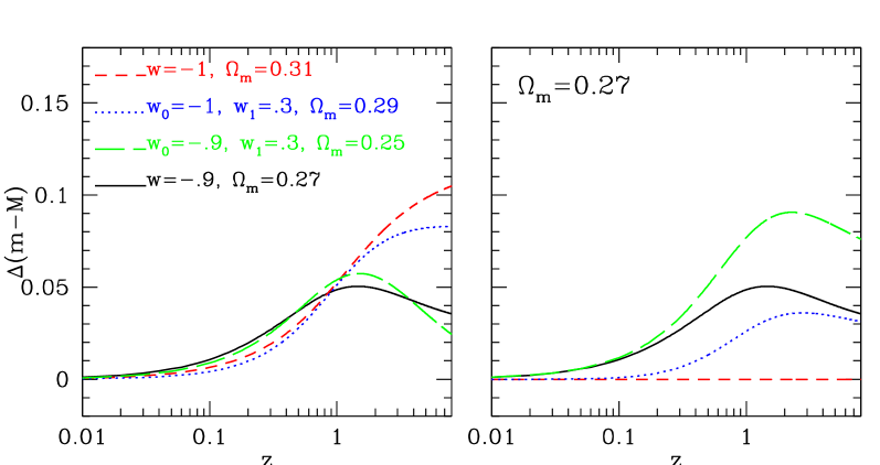
Figure 1: Left Panel: The expected distance modulus difference between the dark-energy models shown and the reference $\Lambda$-model ($w=-1$) with $\Omega_{m}=0.27$. Right Panel: The expected distance modulus differences once the $\Omega_{m}$-$w(z)$ degeneracy is broken (imposing the same $\Omega_{m}$ value as the comparison model).

Three important observations should be made from Figure 1:

1. The relative magnitude deviations between the different dark-energy models are quite small (typically $\raise-3.0pt\hbox{\hbox to0.0pt{\hbox{$\sim$}\hss}\raise 4.0pt\hbox{$<$}\ }0.1$ mag), which puts severe pressure on the necessary photometric accuracy of the relevant observations.

2. The largest relative deviations of the distance moduli occur at redshifts $z\raise-3.0pt\hbox{\hbox to0.0pt{\hbox{$\sim$}\hss}\raise 4.0pt\hbox{$>$}\ }1.5$, and thus at quite larger redshifts than those currently traced by SN Ia, and

3. There are strong degeneracies between the different cosmological models at redshifts $z\raise-3.0pt\hbox{\hbox to0.0pt{\hbox{$\sim$}\hss}\raise 4.0pt\hbox{$<$}\ }1$, but in some occasions even up to much higher redshifts (one such example is shown in Figure 1 between the models with $(\Omega_{m},w_{0},w_{1})=(0.31,-1,0)$ and $(0.29,-1,0.2)$.

Luckily, such degeneracies can be broken, as discussed already in the introduction, by using other cosmological tests (eg. the clustering of extragalactic sources, the CMB shift parameter, BAO’s, etc). Indeed, current evidence overwhelmingly show that the total matter content of the universe is within the range: $0.2\raise-3.0pt\hbox{\hbox to0.0pt{\hbox{$\sim$}\hss}\raise 4.0pt\hbox{$<$}\ }\Omega_{m}\raise-3.0pt\hbox{\hbox to0.0pt{\hbox{$\sim$}\hss}\raise 4.0pt\hbox{$<$}\ }0.3$, a fact that reduces significantly the degeneracies between the cosmological parameters.

2.2 Larger numbers or higher redshifts ?

In order to define an efficient strategy to put stringent constraints on the dark-energy equation of state, we have decided to re-analyse two recently compiled SNIa samples, the Davies et al. (2007) [hereafter D07] compilation of 192 SNIa (based on data from Wood-Vasey et al. 2007, Riess et al. 2007 and Astier et al. 2007) and the UNION compilation of 307 SNIa (Kowalski et al. 2008). Note that the two samples are not independent since most of the D07 is included in the UNION sample.

Firstly, we present in the left panel of Figure 2 the UNION SNIa distance moduli overploted (red-line) with the theoretical expectation of a flat cosmology with $(\Omega_{m},w)=(0.27,-1)$. In the right panel we plot the distance moduli difference between the SNIa data and the previously mentioned model. To appreciate the level of accuracy needed in order to put constraints on the equation of state parameter, we also plot the distance moduli difference between the reference $(\Omega_{m},w)=(0.27,-1)$ and the $(\Omega_{m},w)=(0.27,-0.85)$ models (thin blue line).

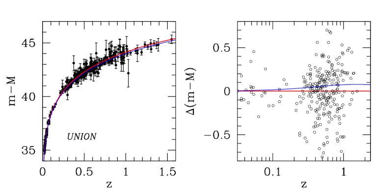
Figure 2: Left Panel: SNIa distance moduli as a function of redshift. Right Panel: Distance moduli difference between the $\Lambda$-model and the SNIa data. The blue line is the corresponding difference between the reference ($w=-1$) and the $w=-0.85$ dark-energy models.

We proceed to analyse the SNIa data by defining the usual likelihood estimator as:

$${\cal L}^{\rm SNIa}({\bf c})\propto{\rm exp}[-\chi^{2}_{\rm SNIa}({\bf c})/2]$$ (6)

where ${\bf c}$ is a vector containing the cosmological parameters that we want to fit for, and

$$\chi^{2}_{\rm SNIa}({\bf c})=\sum_{i=1}^{N}\left[\frac{\mu^{\rm th}(z_{i},{\bf c})-\mu^{\rm obs}(z_{i})}{\sigma_{i}}\right]^{2}\;\;,$$ (7)

where $\mu^{\rm th}$ is given by eq.(3), $z_{i}$ is the observed redshift and $\sigma_{i}$ the observed distance modulus uncertainty. Here we will constrain our analysis within the framework of a flat ($\Omega_{\rm tot}=1$) cosmology and therefore the corresponding vector ${\bf c}$ is: ${\bf c}\equiv[\Omega_{m},w_{0},w_{1}]$. We will use only SNIa with $z>0.02$ in order to avoid possible problems related to redshift uncertainties due to the local bulk flow.

• Larger Numbers? The first issue that we wish to address is how better have we done in imposing cosmological constraints by increasing the available SNIa sample from 181 to 292 (excluding the $z<0.02$ SNIa), ie., increasing the sample by more than 60%. In Table 1 we present various solutions using each of the two previously mentioned samples. Note that since only the relative distances of the SNIa are accurate and not their absolute local calibration, we always marginalize with respect to the internally derived Hubble constant (note that fitting procedures exist which do not need to a priori marginalize over the internally estimated Hubble constant; eg., Wei 2008).

  

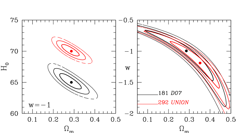
  Figure 3: Solution space of the fits to the Cosmological parameters using either of the two SNIa data sets. The contours are plotted where $-2{\rm ln}{\cal L}/{\cal L}_{\rm max}$ is equal to 2.30, 6.16 and 11.83, corresponding to 1$\sigma$, 2$\sigma$ and 3$\sigma$ confidence level.

  We present our results in Figure 3. The left panel shows the internally derived Hubble constant for each of the to samples (and for $w=-1$). It is evident that the derived values, which we use to free our analysis of the $H_{0}$ dependence of the distance modulus, are well constrained ($h_{0}=0.6515\pm 0.007$ and $0.7015\pm 0.005$ for the D07 and UNION sample, respectively). The right panel shows the main results of interest. The size of the well-known banana shape region of the ($\Omega_{m},w$) solution space is almost identical for both samples of SNIa.

  A first conclusion is therefore that the increase by $\sim 60\%$ of the UNION sample has not provided more stringent constraints to the cosmological parameters. Rather there appears to be an unexpected lateral shift of the contours towards higher values of $\Omega_{m}$ and lower values of $w$, within, however, the 1 $\sigma$ contour of the solution space. In order to verify that the larger number of SNIa’s in the UNION sample are not preferentially located at low-$z$’s - in which case we should have not expected more stringent cosmological constraints using the latter SNIa sample - we plot in Figure 4 the normalized redshift frequency distributions of the two samples (left panel) and the relative increase of SNIa’s as a function of redshift in the UNION sample with respect to the D07 sample in the right panel. It is evident that the larger number of UNION SNIa’s are distributed in all redshifts, except for $z\raise-3.0pt\hbox{\hbox to0.0pt{\hbox{$\sim$}\hss}\raise 4.0pt\hbox{$>$}\ }1$, where there is no appreciable increase of SNIa numbers.

  

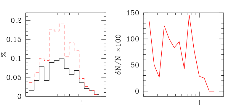
  Figure 4: Redshift distribution of the UNION and D07 SNIa’s (left panel) and the relative increase of SNIa numbers (in percent) between the two samples.

  Table 1: Fitting the SNIa data (with $z>0.02$ in order to avoid local bulk flow effects) to flat cosmologies. Note that for the case where ${\bf c}=(\Omega_{m},w)$ (ie., last row), the errors shown are estimated after marginalizing with respect to the other fitted parameter.

  	D07			UNION
  free params	$w$	$\Omega_{m}$	$\chi^{2}_{\rm min}$/df	$w$	$\Omega_{m}$	$\chi^{2}_{\rm min}$/df
  $\Omega_{m}$	${\bf-1}$	$0.280^{+0.025}_{-0.015}$	187.03/180	${\bf-1}$	$0.280^{+0.020}_{-0.015}$	301.93/291
  $\Omega_{m},w$	$-1.025^{+0.060}_{-0.045}$	$0.292\pm 0.018$	187.02/179	$-1.212\pm 0.050$	$0.355\pm 0.015$	301.11/290

  We already have a strong hint, from the previously presented comparison between the D07 and UNION results, that increasing the number of Hubble relation tracers, covering the same redshift range and with the current level of uncertainties as the available SNIa samples, appears to be a futile avenue in constraining further the cosmological parameters.

• Lower uncertainties or higher-$z$’s: We now resort to a Monte-Carlo procedure which will help us investigate which of the following two directions, which bracket many different possibilities, would provide more stringent cosmological constraints:

  • Reduce significantly the distance modulus uncertainties of SNIa, tracing however the same redshift range as the currently available samples, or

  • use tracers of the Hubble relation located at redshifts where the models show their largest relative differences ($z\raise-3.0pt\hbox{\hbox to0.0pt{\hbox{$\sim$}\hss}\raise 4.0pt\hbox{$>$}\ }2$), with distance modulus uncertainties comparable to that of the highest redshift SNIa’s ($\langle\sigma_{\mu}\rangle\simeq 0.4$)

  The Monte-Carlo procedure is based on using the observed high-$z$ SNIa distance modulus uncertainty distribution ($\sigma_{\mu}$) and a model to assign random $\mu$-deviations from a reference $H(z)$ function, that reproduces exactly the banana-shaped contours of the $(\Omega_{m},w)$ solution space of Figure 3 (right panel). Indeed, after a trial and error procedure we have found that by assigning to each UNION SNIa (using only their redshift) a distance modulus deviation ($\delta\mu$) from the reference model (in this case we use: $\Omega_{m}=0.35,w=-1.21$), using a Gaussian with zero mean and variance given by observed $\langle\sigma_{\mu}\rangle^{2}$), and using as the relevant individual distance modulus uncertainty, which enters as a weight in the $\chi^{2}$ of eq.8, the following: $\sigma^{2}_{i}=\sqrt{(1.1\delta\mu_{i})^{2}+\phi^{2}}$, with $\phi$ a random Poisson deviate within $[-0.01,0.01]$, we reproduce exactly the banana-shaped solution range of the reference model (details will appear elsewhere). This can be seen clearly in the upper left panel of Figure 5, where we plot the original UNION solution space (black contours) and the model solution space (red contours). In the right panel we show the distribution of the true SNIa deviations from the best fitted model (Table 1) as well as a random realization of the model deviations.

  

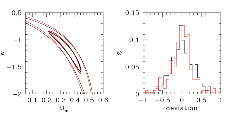
  Figure 5: Left Panel: Comparison between the UNION SNIa constraints (black contours) and those derived by a Monte-Carlo procedure designed to closely reproduce them (for clarity we show only contours corresponding to 1 and 3 $\sigma$ confidence levels). Right Panel: The UNION SNIa distance modulus deviations from the best fit model - $(\Omega_{m},w)=(0.35,-1.21)$ - and a random realization of the model deviations (see text).

  Armed with the above procedure we can now address the questions posed previously. Firstly, we reduce to half the random deviations of the SNIa distance moduli from the reference model (with the corresponding reduction of the relevant uncertainty, $\sigma_{i}$). The results of the likelihood analysis can be seen in the left panel of Figure 6. There is a reduction of the range of the solution space, but indeed quite a small one. Secondly, we have increase artificially the high-$z$ tracers by 88 objects (by additionally using the $z>0.65$ SNIa and adding a $\delta z=2$ to their redshift). Note that the new tracers are distributed between $2.65\raise-3.0pt\hbox{\hbox to0.0pt{\hbox{$\sim$}\hss}\raise 4.0pt\hbox{$<$}\ }z\raise-3.0pt\hbox{\hbox to0.0pt{\hbox{$\sim$}\hss}\raise 4.0pt\hbox{$<$}\ }3.55$, ie., in a range where the largest deviations between the different cosmological models occur (see Figure 1). The deviations from the reference model of these additional SNIa are based on their original $\mu$ uncertainty distribution (ie., we have assumed that the new high-$z$ tracers will have similar uncertainties as their $z\raise-3.0pt\hbox{\hbox to0.0pt{\hbox{$\sim$}\hss}\raise 4.0pt\hbox{$>$}\ }0.65$ counterparts, which is $\langle\sigma_{\mu}\rangle\simeq 0.38$). We now find a significantly reduced solution space (right panel of Figure 6), which shows that indeed by increasing the $H(z)$ tracers by a few tens, at those redshifts where the largest deviations between models occur, can have a significant impact on the recovered cosmological parameter solution space.

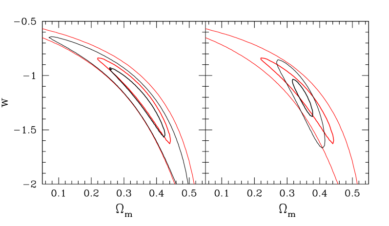
Figure 6: Comparison of the present SNIa constraints (red contours) with Left Panel: those derived by reducing to half their uncertainties (black contours) and Right Panel: with those derived by adding a sample of 88 high-$z$ tracers ($2.5\raise-3.0pt\hbox{\hbox to0.0pt{\hbox{$\sim$}\hss}\raise 4.0pt\hbox{$<$}\ }z\raise-3.0pt\hbox{\hbox to0.0pt{\hbox{$\sim$}\hss}\raise 4.0pt\hbox{$<$}\ }3.6$) with a distance modulus mean uncertainty of $\sigma_{\mu}\simeq 0.38$ (black contours).

The main conclusion of the previous analysis is that the best strategy to decrease the uncertainties of the cosmological parameters based on the Hubble relation is to use standard candles which trace also the redshift range $2\raise-3.0pt\hbox{\hbox to0.0pt{\hbox{$\sim$}\hss}\raise 4.0pt\hbox{$<$}\ }z\raise-3.0pt\hbox{\hbox to0.0pt{\hbox{$\sim$}\hss}\raise 4.0pt\hbox{$<$}\ }4$. Below we present such a possibility by suggesting an alternative to the SNIa standard candles, namely HII-like starburst galaxies (eg. Melnick 2003; Siegel et al. 2005).

2.3 Hubble Relation using HII-like starburst galaxies

We now reach our suggestion to use an alternative and potentially very powerful technique to estimate cosmological distances, which is the relation between the luminosity of the $H_{\beta}$ line and the stellar velocity dispersion, measured from the line-widths, of HII regions and galaxies (Terlevich & Melnick 1981, Melnick, Terlevich & Moles 1988). The cosmological use of this distance indicator has been tested in Melnick, Terlevich & Terlevich (2000) and Siegel et al (2005) (see also the review by Melnick 2003). It is the presence of O and B-type stars in HII regions that causes the strong Balmer line emission, in both $H_{\alpha}$ and $H_{\beta}$. Furthermore, the fact that the bolometric luminosities of HII galaxies are dominated by the starburst component implies that their luminosity per unit mass is very large, despite the fact that the galaxies are low-mass. Therefore they can be observed at very large redshifts, and this fact makes them cosmologically very interesting objects. Furthermore, it has been shown that the $L(H_{\beta})-\sigma$ correlations holds at large redshifts (Koo et al. 1996, Pettini et al. 2001, Erb et al. 2003) and therefore they can be used to trace the Hubble relation at cosmologically interesting distances. One of the most important prerequisites in using such relations, as distance estimators, is the accurate determination of their zero-point. To this end, Melnick et al (1988) used giant HII regions in nearby late-type galaxies and derived the following empirical relation (using a Hubble constant of $H_{0}=71$ km/sec/Mpc):

$$\log L(H_{\beta})=\log M_{z}+29.60\;\;{\rm with}\;\;M_{z}=\sigma^{5}/(O/H)$$ (8)

where $O/H$ is the metallicity. Based on the above relation and the work of Melnick, Terlevich & Terlevich (2000), the distance modulus of HII galaxies can be derived from:

$$\mu=2.5\log(\sigma^{5}/F_{H\beta})-2.5\log(O/H)-A_{H\beta}-26.44$$ (9)

with $F_{H\beta}$ and $A_{H\beta}$ are the flux and extinction in $H_{\beta}$. The rms dispersion in distance modulus was found to be $\sim 0.52$ mag. The analysis of Melnick, Terlevich & Terlevich (2000) has shown that most of this dispersion ($\sim 0.3$ mags) comes from observational errors in the stellar velocity dispersion measurements, from photometric errors and metallicity effects. It is therefore important to understand and correct the sources of random and systematic errors of the $L(H_{\beta})-\sigma$ relation, and indeed with the availability of new observing techniques and instruments, we hope to reduce significantly the previously quoted rms scatter.

A few words are also due to the possible systematic effects of the above relation. Such effects may be related to the age of the HII galaxy (this can be dealt with by putting a limit in the equivalent width of the $H_{\beta}$ line, eg. $EW(H_{\beta})>$ 25 Angs; see Melnick 2003), to extinction, to different metallicities and environments. Also the $EW(H_{\beta})$ of HII-like galaxies at intermediate and high redshifts are smaller than the local ones, a fact which should be taken into account.

We have commenced an investigation of all these effects by using high-resolution spectroscopy of a relatively large number of SDSS low-$z$ HII galaxies, with a range of $H_{\beta}$ equivalent widths, luminosities, metal content and local overdensity, in order to reduce the scatter of the HII-galaxy based distance estimator to about half its present value, ie., our target is $\sim 0.25$ mag. We will also define a medium and high redshift sample (see Pettini et al. 2001; Erb et al. 2003), consisting of a few hundred objects distributed in the different high-redshift bins, which will finally be used to define the high-$z$ Hubble function.

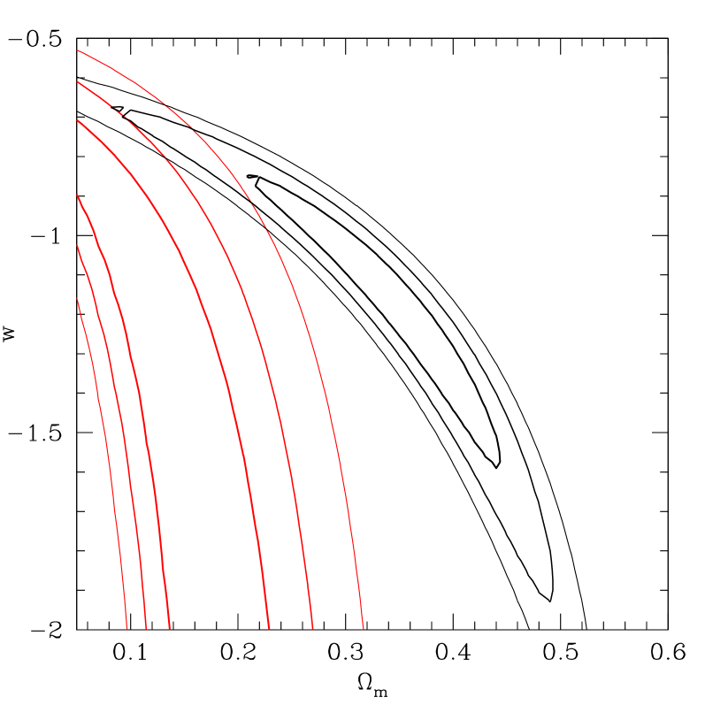
Figure 7: Comparison between the UNION SNIa constraints and those derived by using the 15 high-$z$ starburst galaxies of Siegel et al. (2005). Although, the latter constraints are weak and mostly inconsistent with the former, this plot serves to indicate the potential of using high-$z$ starburst galaxies (once of course we have reduced significantly their distance modulus uncertainties).

Summarizing, the use of HII galaxies to trace the Hubble relation, as an alternative to the traditionally used SN Ia, is based on the following facts:

• local and high-$z$ HII-like galaxies and HII regions are physically very similar systems (Melnick et al 1987) providing a phenomenological relation between the luminosity of the $H_{\beta}$ line, the velocity dispersion and their metallicity as traced by $O/H$ (Melnick, Terlevich & Moles 1988). Therefore HII-like starburst galaxies can be used as alternative standard candles (Melnick, Terlevich & Terlevich 2000, Melnick 2003; Siegel et al. 2005)

• such galaxies can be readily observed at much larger redshifts than those currently probed by SNIa and

• it is at such higher redshifts that the differences between the predictions of the different cosmological models appear more vividly.

Already a sample of 15 such high-z starburst galaxies have been used by Siegel et al. (2005) in an attempt to constrain cosmological parameters but the constraints, although in the correct direction, are very weak. Here we perform our own re-analysis of this data-set and the resulting constraints on the $\Omega_{m},w$ plane (for a flat geometry) can be seen in Figure 7. Note that imposing $w=-1$, our analysis of the Siegel et al (2005) data set provides $\Omega_{m}=0.10\pm 0.05$, which is towards the lower side of the generally accepted values. Comparing these HII-based results to the present constraints of the latest SNIa data (D07 and UNION) clearly indicates the necessity to:

• re-estimate carefully the local zero-point of the $L(H_{\beta})-\sigma$ relation,

• suppress the HII-galaxy distance modulus uncertainties,

• increase the high-$z$ starburst sample by a large fraction,

• make sure to select high-$z$ bona-fide HII-galaxies, excluding those that show indications of rotation (Melnick 2003).

3 The Clustering of high-z X-ray AGN

X-ray selected AGNs provide a relatively unbiased census of the AGN phenomenon, since obscured AGNs, largely missed in optical surveys, are included in such surveys. Furthermore, they can be detected out to high redshifts and thus trace the distant density fluctuations providing important constraints on super-massive black hole formation, the relation between AGN activity and Dark Matter (DM) halo hosts, the cosmic evolution of the AGN phenomenon (eg. Mo & White 1996, Sheth et al. 2001), and on cosmological parameters and the dark-energy equation of state (eg. Basilakos & Plionis 2005; 2006).

The earlier ROSAT-based analyses (eg. Boyle & Mo 1993; Vikhlinin & Forman 1995; Carrera et al. 1998; Akylas, Georgantopoulos, Plionis, 2000; Mullis et al. 2004) provided conflicting results on the nature and amplitude of high-$z$ AGN clustering. With the advent of the XMM and Chandra X-ray observatories, many groups have attempted to settle this issue, but in vain. Different surveys have provided again a multitude of conflicting results, intensifying the debate (eg. Yang et al. 2003; Manners et al. 2003; Basilakos et al. 2004; Gilli et al. 2005; Basilakos et al 2005; Yang et al. 2006; Puccetti et al. 2006; Miyaji et al. 2007; Gandhi et al. 2006; Carrera et al. 2007). However, the recent indications of a flux-limit dependent clustering appears to remove most of the above inconsistencies (Plionis et al. 2008; see also Figure 8).

Figure 8: The angular correlation scale, $\theta_{0}$, as a function of different survey characteristic flux, defined as that corresponding to half the respective survey area-curves. Most results appear to be consistent with the clustering flux-limit dependence, found from the CDF-N and CDF-S (from Plionis et al. 2008).

Furthermore, there are indications for a quite large high-$z$ AGN clustering length, reaching values $\sim 15-18\;h^{-1}$ Mpc at the brightest flux-limits (eg., Basilakos et al 2004; 2005, Puccetti et al. 2006, Plionis et al. 2008), a fact which, if verified, has important consequences for the AGN bias evolution and therefore for the evolution of the AGN phenomenon (eg. Miyaji et al. 2007; Basilakos, Plionis & Ragone-Figueroa 2008). An independent test of these results will be to establish that the environment of high-$z$ AGN is associated with large DM haloes, which being massive should be more clustered.

Below we justify the necessity for a large-area XMM survey in order to unambiguously determine the clustering pattern of high-$z$ ($z\sim 1$) X-ray AGNs. We further show that such measurements can be used to put strong cosmological constraints (see for example Basilakos & Plionis 2005; 2006), and help break the $\Omega_{m},w$ degeneracies.

3.1 Biases and Systematics:

It is important to understand and overcome the shortcomings and problems that one is facing in order to reliably and unambiguously determine the clustering properties of the X-ray selected AGNs. Below we list the source of such problems, some of which can be rectified by considerably increasing the X-ray survey area.

• Cosmic Variance: Is the volume surveyed large enough to smooth out inhomogeneities of the large-scale distribution of AGNs? (for example see Stewart et al. 2007). Closely related to this problem is the so-called integral constraint, which practically depends on the unknown true mean density of the cosmic sources under study. If the area is small enough, then the mean density, estimated from the survey itself, is way-out of its true value and thus the usual correlation function analysis will impose the observed mean number density as the true one (an example of this is the CDF-S were a large number of superclusters at $z\sim 0.7$ are found; see Gilli et al. 2003). This usually results into an underestimation of the true correlation amplitude and a shallower zero-crossing of the estimated $\xi(r)$ or $w(\theta)$. A source of the observed scatter between the presently available surveys (see Figure 8) could well be the cosmic variance. These problems, however, are rectified with the large-area XMM survey proposed.

• The amplification bias which can enhance artificially the clustering signal due to the detector’s PSF smoothing of source pairs with intrinsically small angular separations (see Vikhlinin & Forman 1995; Basilakos et al. 2005). This problem can affect clustering results if at the median redshift of the sources under study the XMM PSF angular size corresponds to a rest-frame spatial scale comparable to the typical source pair-wise separations. Furthermore, the possible variability of the PSF size through-out the XMM fields can have an additional effect. This should be modeled and tested with Monte-Carlo simulations in order to establish the extent to which the clustering results are affected. In large-area surveys it is necessary to take good-care of this effect when using source pairs that belong to different XMM pointings.

• Reliable production of random source catalogues: This is an issue which is extremely important and not appreciated at the necessary extent. The random catalogues, with which the observed source-pairs are compared, should be produced to account for all systematic effects from which the observations suffer, among which the different positional sensitivity and edge effects of each XMM pointing. Furthermore, a reliable $\log N-\log S$ distribution (theoretically motivated or observationally determined) should be reproduced in the random “XMM pointings” and the random sources should be observed following the same procedure as in the true observations. Random positioned sources with fluxes lower than that corresponding to the particular position of the sensitivity map of the particular XMM pointing should be removed from each random catalogue.

An optimal approach to unambiguously determine the clustering pattern of X-ray selected AGNs would be to determine both the angular and spatial clustering pattern. The reason being that various systematic effects or uncertainties enter differently in the two types of analyses. On the one side, using $w(\theta)$ and its Limber inversion, one by-passes the effects of redshift-space distortions and uncertainties related to possible misidentification of the optical counter-parts of X-ray sources. On the other side, using spectroscopic or accurate photometric redshifts to measure $\xi(r)$ or $w_{p}(\theta)$ one by-passes the inherent necessity, in Limber’s inversion of $w(\theta)$, of the source redshift-selection function (for the determination of which one uses the integrated X-ray source luminosity function, different models of which exist). For the inversion to work it is also necessary to model the spatial correlation function as a power law, to assume a clustering evolution model, which is taken usually to be that of constant clustering in comoving coordinates (eg. de Zotti et al. 1990; Kundić 1997) and also to assume a cosmological model. Limber’s inversion then reads:

$$\theta_{\circ}^{\gamma-1}=H_{\gamma}r_{\circ}^{\gamma}\left(\frac{H_{\circ}}{c}\right)^{\gamma}\int_{0}^{\infty}\left(\frac{1}{N}\frac{{\rm d}N}{{\rm d}z}\right)^{2}\frac{E(z)}{x^{\gamma-1}(z)}{\rm d}z\;,$$ (10)

where $\epsilon=\gamma-3$ for the constant clustering in comoving coordinates model, $x(z)$ is the proper distance, $E(z)=\sqrt{\Omega_{\rm m}(1+z)^{3}+\Omega_{\Lambda}}$ and $H_{\gamma}=\Gamma(\frac{1}{2})\Gamma(\frac{\gamma-1}{2})/\Gamma(\frac{\gamma}{2})$. As noted previously, for the inversion to be possible it is necessary to know the X-ray source redshift distribution, ${\rm d}N/{\rm d}z$, and the total number, $N$, of the X-ray sources, which can be determined by integrating the X-ray source luminosity function above the minimum luminosity that corresponds to the particular flux-limit used.

3.2 X-ray surveys

In order to reach a flux-limit for which the soft-band clustering appears to converge to its final value (due to the flux-limit-clustering correlation, revealed in Plionis et al. 2008; see also Figure 8) we plan to analyse all $>$10 ksec XMM pointings, which will allow us to reach a flux-limit of $\sim 2\times 10^{-15}$ erg/sec/cm² in the soft (0.5-2 keV) and $\sim 10^{-14}$ erg/sec/cm² in the hard (2-10 keV) bands, respectively. Such an exposure time will finally provide (taking in to account realistci observational effects) $\sim$250 soft-band and $\sim$100 hard-band X-ray sources per deg², according to the Kim et al. (2007) $\log N-\log S$ and since all publicly available XMM pointings, with exposure time more than 10 ksec, add to $\sim 300$ non-contiguous sq.degrees, implies a resulting sample of $\sim 75000$ soft and $\sim 30000$ hard X-ray sources. These numbers will allow us to derive with great accuracy the small-separation angular correlation function, the Limber’s inversion of which can provide their spatial correlation function. Furthermore, around 100 non-contiguous sq.degrees of the previous survey (except for a few contiguous regions with areas between 2 and 10 sq.degrees each) are covered also by the SDSS, providing crude photo-$z$’s. This will allow us to derive the angular correlation function in distinct redshift bins in the range $0.5<z<2$ and thus quantify the evolution of the bias of X-ray selected AGN, an important ingredient in disentangling the cosmological parameters. Note finally that $\sim$50 sq.degrees are covered also by the publicly available UKIDSS (http://www.ukidss.org/) which provide 3 near-IR colours and thus for a subsample of the previous data we will have relatively more accurate photo-$z$’s allowing us to attempt to derive directly the spatial correlation function.

Summarizing, the analysis of such large XXM surveys will allow us to unambiguously determine the soft and hard-band X-ray AGN clustering pattern, minimizing the biases and systematic effects discussed in the previous section, as well as to study the evolution of the AGN correlation function (utlizing photo-$z$’s and dividing the angular sample into 2-3 $z$-bins).

Finally, together with a large European consortium, we are planning to survey a 2-3 contiguous sky areas adding to $\sim 50$ deg² and covered also by a large number of other multiwavelength surveys (like UKIDSS, NEWFIRM, etc), which will probably allow us to sample the long wavelength regime of the AGN correlation function, and thus measure Baryonic Accoustic Oscillations, which are extremely important for Dark-energy investigations (Peacock et al 2006; Albrecht et al. 2006). To obtain the necessary high photo-$z$ accuracy, one may envision a wide-field multi-filter (say using $\sim$20 broad and narrow-band filters) survey, specially tuned in order to obtain relatively high-accuracy photo-$z$’s of $z\sim 1$ AGN. Thoughts for the aquisition of such an instrument, to be mounted on the 2.3m Hellenic Aristarchos telescope, are already been discussed in the Institute of Astronomy & Astrophysics of the National Observatory of Athens.

3.3 Cosmological Parameter constraints from X-ray AGN Clustering

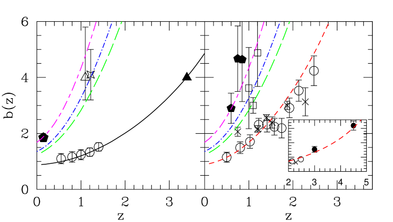
Figure 9: Comparison of the Basilakos et al (2008) $b(z)$ evolution model with different observational data. Different line types represent different halo masses. Left Panel: optical galaxies (open points) with solid line corresponding to $M_{\rm DM}\sim 10^{12}\;h^{-1}\;M_{\odot}$, Lyman break galaxies (solid triangle), EROs (star), DRGs (open triangle) and 2dF radio sources (filled pentagon). The dot-dashed line corresponds to 7.7 $\times 10^{13}\;h^{-1}\;M_{\odot}$. Right Panel: optically selected quasars (open points and crosses), soft and hard X-ray point sources (open squares and solid diamonds; the large scatter corresponds to the uncertainty of the present day clustering results; see Plionis et al. 2008 and references therein). In the insert we plot, as solid points, the high-$z$ SSRS DR5 QSOs and the same $b(z)$ model that fits their lower redshift counterparts (ie., $M_{\rm DM}\simeq 10^{13}\;h^{-1}\;M_{\odot}$).

The unambiguous determination of the correlation function of the $z\sim 1$ X-ray AGNs, even in angular space, will allow us to estimate with good precision (a) their relation to the underlying matter fluctuations at $z\sim 1$ (ie., their bias), (b) the evolution of their bias and therefore the mass of the DM haloes which they inhabit (eg., Miyaji et al. 2007; Basilakos, Plionis & Ragone-Figueroa 2008) and (c) put strong cosmological constraints on the $\Omega_{m},h$ or $\Omega_{m},\sigma_{8}$ planes, while with the help of the high-$z$ HII-based Hubble relation on the $\Omega_{m},w(z)$ space.

It is well known (Kaiser 1984; Benson et al. 2000) that according to linear biasing the correlation function of the AGN (or any mass-tracer) ($\xi_{\rm AGN}$) and dark-matter one ($\xi_{\rm DM}$), are related by:

$$\xi_{\rm AGN}(r,z)=b^{2}(z)\xi_{\rm DM}(r,z)\;\;,$$ (11)

where $b(z)$ is the bias evolution function (eg. Mo & White 1996, Matarrese et al. 1997, Basilakos & Plionis 2001; 2003; Basilakos, Plionis & Ragone-Figueroa 2008)

A first outcome of the proposed correlation function analysis will be the accurate determination of the AGN bias at their median redshift (in our case $\bar{z}\simeq 1$), utilizing:

$$b(z)=\left(\frac{r_{0}}{r_{0,m}}\right)^{\gamma/2}D^{3+\epsilon}(z)\;\;\;\mbox{with}\;\gamma=1.8\;{\rm and}\;\;\epsilon=-1.2\;,$$

where $r_{0}$ and $r_{0,m}$ are the measured AGN and dark-matter (from the $P(k)$) clustering lengths, respectively, while $D(z)$ is the perturbation’s linear growing mode. Then using a bias evolution model, one will be able to determine the mass of the DM halo within which such AGN live (eg. see Figure 9).

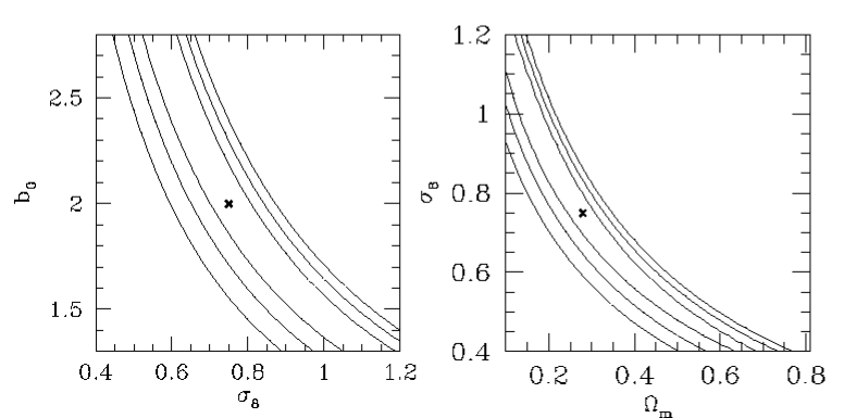
Figure 10: Likelihood contours from the X-ray AGN clustering analysis of Basilakos & Plionis (2005) in the following planes: $(\Omega_{m},\sigma_{8})$ (right panel), $(\sigma_{8},b_{0})$ (left panel). The contours plotted correspond to 1$\sigma$, 2$\sigma$ and 3$\sigma$ confidence level.

Furthermore, we will compare the observed AGN clustering with the predicted, for different cosmological models, correlation function of the underlying mass, $\xi_{\rm DM}(r,z)$. To this end we can use the Fourier transform of the spatial power spectrum $P(k)$:

$$\xi_{\rm DM}(r,z)=\frac{(1+z)^{-(3+\epsilon)}}{2\pi^{2}}\int_{0}^{\infty}k^{2}P(k)\frac{{\rm sin}(kr)}{kr}{\rm d}k\;\;,$$ (12)

where $k$ is the comoving wavenumber, $P(k)=P_{0}k^{n}T^{2}(k)$ the CDM power-spectrum with scale-invariant ($n=1$) primeval inflationary fluctuations, while the transfer function parameterization is as in Bardeen et al. (1986), with the corrections given approximately by Sugiyama (1995).

Basilakos & Plionis (2005; 2006) have already used succesfully a standard maximum likelihood procedure to compare the measured XMM source angular correlation function from a relatively small ($\sim 2$ sq.degrees survey; Basilakos et al. 2005) with the prediction of different spatially flat cosmological models, and derived interesting cosmological contraints (for flat and constant-$w$ cosmologies).

In Figure 10 we present the constraints provided from the preliminary analysis by Basilakos & Plionis (2006) of a $\sim 2$ sq.degrees XMM survey, on the present bias-factor ($b_{0}$) of the X-ray AGN, on the normalization of the power spectrum ($\sigma_{8}$) and on $\Omega_{m}$ (marginalizing over different parameters). In Figure 11 (left panel) we present the $(\Omega_{m},w)$ constraints provided by the X-ray AGN clustering analysis (red contours), once we have marginalized over the $\sigma_{8}(\sim 0.8)$ and the bias factor at the present time ($\sim 2$).

4 Joint Hubble-relation and Clustering analysis

It is evident from Figure 11 (left panel) that $w$ is degenerate with respect to $\Omega_{m}$ and that all the values in the interval $-2\leq w\leq-0.35$ are acceptable within the $1\sigma$ uncertainty. However, we break this degeneracy by adding the constraints provided by the Hubble relation technique, using here the UNION SNIa sample. We therefore perform a joint likelihood analysis, assuming that the two data sets are independent (which indeed they are) and thus we can write the joint likelihood as the product of the two individual ones.

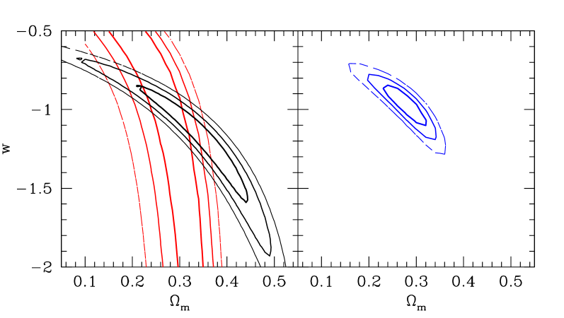
Figure 11: Left Panel: Likelihood contours on the $\Omega_{m},w$ plane from the X-ray AGN clustering analysis of Basilakos & Plionis (2005; 2006) (red contours) and the UNION SNIa analysis (black contours). Right Panel: The Joint likelihood contours.

Our current joint likelihood analysis, once we impose $h=0.72$ and $\sigma_{8}=0.8$, provides quite stringent constraints of the $\Omega_{m}$ and $w$ parameters:

$$\Omega_{\rm m}=0.28^{+0.02}_{-0.04}\;\;\;\;{\rm and}\;\;\;\;w=-1.0\pm 0.1\;.$$

However, the uncertainty on $w$ is still quite large, while the necessity to impose constraints on a more general, time-evolving, dark-energy equation of state (eq. 2) implies that there is ample space for great improvment and indeed the aim of the project, detailed in these proceedings, is exactly in this direction.

References

References

- [1] Akylas, A., Georgantopoulos, I., Plionis, M., 2000, MNRAS, 318, 1036
- [2] Albrecht, A., et al., 2006, astro-ph/0609591
- [3] Allen, S. W., et al., 2004, MNRAS, 353, 457
- [4] Andernach, H., et al., 2005, ASPC, 329, 289
- [5] Antonucci, R., 1993, ARA&A, 31, 473
- [6] Astier, P., et al., 2006, A&A, 447, 31
- [7] Bardeen, J.M., Bond, J.R., Kaiser, N. & Szalay, A.S., 1986, ApJ, 304, 15
- [8] Basilakos, S. & Plionis, M., 2001, ApJ, 550, 522
- [9] Basilakos, S. & Plionis, M., 2003, ApJ, 593, L61
- [10] Basilakos, S., Georgakakis, A., Plionis, M., Georgantopoulos, I., 2004, ApJ, 607, L79
- [11] Basilakos, S., Plionis, M., Georgantopoulos, I., Georgakakis, A., 2005, MNRAS, 356, 183
- [12] Basilakos, S. & Plionis, M., 2005, MNRAS, 360, L35
- [13] Basilakos, S. & Plionis, M., 2006, ApJ, 650, L1
- [14] Basilakos, S., Plionis, M. & Ragone-Figueroa, C., 2008, ApJ, 678, 627
- [15] Basilakos, S. & Perivolaropoulos, L., 2008, MNRAS, 391, 411
- [16] Benson A. J., Cole S., Frenk S. C., Baugh M. C., Lacey G. C., 2000, MNRAS, 311, 793
- [17] Boyle B.J., Mo H.J., 1993, MNRAS, 260, 925
- [18] Blake, C., et al., 2007, MNRAS, 374, 1527
- [19] Carrera, F.J., Barcons, X., Fabian, A. C., Hasinger, G., Mason, K.O., McMahon, R.G., Mittaz, J.P.D., Page, M.J., 1998, MNRAS, 299, 229
- [20] Carrera, F.J., et al. 2007, A&A, 469, 27
- [21] Chevallier M., & Polarski D., 2001, Int. J. Mod. Phys. D, 10, 213
- [22] de Zotti, G., Persic, M., Franceschini, A., Danese, L., Palumbo, G.G.C., Boldt, E.A., Marshall, F.E., 1990, ApJ, 351, 22
- [23] Davis, T.M., et al., 2007, ApJ, 666, 716
- [24] Dicus, D.A. & Repko, W.W., 2004, Phys.Rev.D, 70, 3527,
- [25] Erb, D.K. et al., 2003, ApJ, 591, 101
- [26] Eisenstein, Hu, & Tegmark 1998, ApJ, 504, L57
- [27] Eisenstein et al. 2005, ApJ, 633, 560
- [28] Fabian, A. C., 1991, MNRAS, 253, 29
- [29] Fabian, A., 1999, MNRAS, 308, L39
- [30] Gandhi, P., et al., 2006, A&A, 457, 393
- [31] Gilli, R., et al. 2003, ApJ, 592, 721
- [32] Ghirlanda, G., Ghisellini, G., Firmani, C., 2006, NewJPhys, 8, 123
- [33] Göttlober, S. & Yepes, G., 2007, ApJ, 664, 117
- [34] Kim, M., Wilkes, B.J., Kim, D-W., Green, P.J., Barkhouse, W.A., Lee, M.G., Silverman, J.D., Tananbaum, H.D., 2007, ApJ, 659, 29
- [35] Kaiser N., 1984, ApJ, 284, L9
- [36] Kowalski M. et al., 2008, ApJ, 686, 749
- [37] Kundić, T., 1997, ApJ, 482, 631
- [38] Linder, V. E., 2003, Phys. Rev. Lett., 90, 091301
- [39] Matsubara, T., 2004, ApJ, 615, 573
- [40] Manners, J.C., et al., 2003, MNRAS, 343, 293
- [41] Matarrese, S., Coles, P., Lucchin, F., Moscardini, L., 1997, MNRAS, 286, 115
- [42] Melnick, J., 1978, A&A, 70, 157
- [43] Melnick J., Terlevich, R., Moles, M., 1988, MNRAS, 235, 313;
- [44] Melnick, J., Terlevich, R., Terlevich, E., 2000, MNRAS, 311, 629
- [45] Melnick, J., 2003, Star Formation Through Time’, ASP Conference Proceedings, Vol. 297, Edited by E.Perez, R.M. Gonzalez Delgado & G. Tenorio-Tagle
- [46] Miyaji, T., et al., 2007, ApJS, 172, 396
- [47] Mullis C.R., Henry, J. P., Gioia I. M., Böhringer H., Briel, U. G., Voges, W., Huchra, J. P., 2004, ApJ, 617, 192
- [48] Mo, H.J, & White, S.D.M 1996, MNRAS, 282, 347
- [49] Newman, J. A., et al., 2002, PASP, 114, 29
- [50] Padmanabhan et al. 2007, MNRAS, 378, 852
- [51] Peacock et al., 2006, astro-ph/0610906
- [52] Peebles P.J.E., &, Ratra, B., 2003, RvMP, 75, 559
- [53] Perlmutter, S., et al., 1998, Nature, 391, 51
- [54] Perlmutter, S., et al., 1999, ApJ, 517, 565
- [55] Pettini, M., et al., 2001, ApJ, 554, 981
- [56] Plionis, M., Rovilos, M., Basilakos, S., Georgantopoulos, I., Bauer, F., 2008, ApJ, 674, L5
- [57] Puccetti, S., et al., 2006, A&A, 457, 501
- [58] Ragone-Figueroa C. & Plionis M., 2006, MNRAS, 377, 1785
- [59] Riess, A. G., et al., 1998, AJ, 116, 1009
- [60] Riess, A. G., et al., 2004, ApJ, 607, 665
- [61] Riess A.G., 2007, ApJ, 659, 98
- [62] Rosati, P., et al., 2002, ARA&A, 40, 539
- [63] Sanchez, A. G., et al., 2006, MNRAS, 366, 189
- [64] Schuecker, P., et al., 2003, A&A, 402, 53
- [65] Seljak, U., et al., 2004, Phys.Rev.D, 71, 3515
- [66] Sheth, R.K., Mo, H.J., Tormen, G., 2001, MNRAS, 323, 1
- [67] Siegel, E.R., et al., 2005, MNRAS, 356, 1117
- [68] Spergel, D. N., et al., 2003, ApJS, 148, 175
- [69] Spergel, D.N., et al. 2007, ApJS, 170, 377
- [70] Stewart, G.C., 2007, in ”X-ray Surveys: Evolution of Accretion, Star-Formation and the Large-Scale Structure”, Rodos island, Greece, http://www.astro.noa.gr/xray07/rodos-talks/
- [71] Sugiyama, N., 1995, ApJS, 100, 281
- [72] Tegmark, M., et al., 2004, Phys.Rev.D., 69, 3501
- [73] Terlevich, R., Melnick, J., 1981, MNRAS, 195, 839
- [74] Tonry, et al. , 2003, ApJ, 594, 1
- [75] Vikhlinin, A. & Forman, W., 1995, ApJ, 455, 109
- [76] Yang, Y., Mushotzky, R.F., Barger, A.J., Cowie, L.L., Sanders, D.B., Steffen, A.T., 2003, ApJ, 585, L85
- [77] Yang, Y., Mushotzky, R.F., Barger, A.J., Cowie, L.L., 2006, ApJ, 645, 68
- [78] Vikhlinin, A., et al., 2003, ApJ, 590, 15
- [79] Wang, Y. & Mukherjee, P., 2006, ApJ, 650, 1
- [80] Wei, , H., 2008, astro-ph/0809.0057
- [81] White, S.D.M., et al., 1993, Nature, 366, 429
- [82] Wood-Vasey W.M., et al., 2007, ApJ, 666, 694