Large dimensional random $k$ circulants

Abstract.

Consider random $k$-circulants $A_{k,n}$ with $n\to\infty,k=k(n)$ and whose input sequence $\{a_{l}\}_{l\geq 0}$ is independent with mean zero and variance one and $\sup_{n}n^{-1}\sum_{l=1}^{n}\mathbb{E}|a_{l}|^{2+\delta}<\infty$ for some $\delta>0$. Under suitable restrictions on the sequence $\{k(n)\}_{n\geq 1}$, we show that the limiting spectral distribution (LSD) of the empirical distribution of suitably scaled eigenvalues exists and identify the limits. In particular, we prove the following: Suppose $g\geq 1$ is fixed and $p_{1}$ is the smallest prime divisor of $g$. Suppose $P_{g}=\prod_{j=1}^{g}E_{j}$ where $\{E_{j}\}_{1\leq j\leq g}$ are i.i.d. exponential random variables with mean one.

(i) If $k^{g}=-1+sn$ where $s=1$ if $g=1$ and $s=o(n^{p_{1}-1})$ if $g>1$, then the empirical spectral distribution of $n^{-1/2}A_{k,n}$ converges weakly in probability to $U_{1}P_{g}^{1/2g}$ where $U_{1}$ is uniformly distributed over the $(2g)$th roots of unity, independent of $P_{g}$.

(ii) If $g\geq 2$ and $k^{g}=1+sn$ with $s=o(n^{p_{1}-1})$ then the empirical spectral distribution of $n^{-1/2}A_{k,n}$ converges weakly in probability to $U_{2}P_{g}^{1/2g}$ where $U_{2}$ is uniformly distributed over the unit circle in $\mathbb{R}^{2}$, independent of $P_{g}$.

On the other hand, if $k\geq 2$, $k=n^{o(1)}$ with $\gcd(n,k)=1$, and the input is i.i.d. standard normal variables, then $F_{n^{-1/2}A_{k,n}}$ converges weakly in probability to the uniform distribution over the circle with center at $(0,0)$ and radius $r=\exp(\mathbb{E}[\log\sqrt{E}_{1}])$.

We also show that when $n=k^{2}+1\to\infty$, and the input is i.i.d. with finite $(2+\delta)$ moment, then the spectral radius, with appropriate scaling and centering, converges to the Gumbel distribution.

1. Introduction

For any (random) $n\times n$ matrix $B$, let $\mu_{1}(B),\ldots,\mu_{n}(B)\in\mathbb{C}=\mathbb{R}^{2}$ denote its eigenvalues including multiplicities. Then the empirical spectral distribution (ESD) of $B$ is the (random) distribution function on $\mathbb{R}^{2}$ given by

$$F_{B}(x,y)=n^{-1}\#\Big{\{}j:\mu_{j}(B)\in(-\infty,x]\times(-\infty,y],\ 1\leq j\leq n\Big{\}}.$$

For a sequence of random $n\times n$ matrices $\{B_{n}\}_{n\geq 1}$ if the corresponding ESDs $F_{B_{n}}$ converge weakly (either almost surely or in probability) to a (nonrandom) distribution $F$ in the space of probability measures on $\mathbb{R}^{2}$ as $n\rightarrow\infty$, then $F$ is called the limiting spectral distribution (LSD) of $\{B_{n}\}_{n\geq 1}$. See Bai (1999)[1], Bose and Sen (2007)[6] and Bose, Sen and Gangopadhyay (2009)[4] for description of several interesting situations where the LSD exists and can be explicitly specified.

Another important quantity associated with a matrix is its spectral radius. For any matrix $B$, its spectral radius $\texttt{sp}(B)$ is defined as

$$\texttt{sp}(B):=\max\Big{\{}|\mu|:\mu\ \text{ is an eigenvalue of }B\Big{\}},$$

where $|z|$ denotes the modulus of $z\in\mathbb{C}$. For classical random matrix models such as the Wigner matrix and i.i.d. matrix, the limiting distribution of an appropriately normalized spectral radius is known for the Gaussian entries (see, for example, Forrester(1993)[13], Johansson (2000)[19], Tracy and Widom (2000)[29] and, Johnstone (2001)[20]) which was later extended by Soshnikov[26, 27] to more general entries.

Suppose $\underline{a}=\{a_{l}\}_{l\geq 0}$ is a sequence of real numbers (called the input sequence). For positive integers $k$ and $n$, define the $n\times n$ square matrix

$$A_{k,n}(\underline{a})=\left[\begin{array}[]{cccc}a_{0}&a_{1}&\ldots&a_{n-1}\\ a_{n-k}&a_{n-k+1}&\ldots&a_{n-k-1}\\ a_{n-2k}&a_{n-2k+1}&\ldots&a_{n-2k-1}\\ &&\vdots&\\ \end{array}\right]_{n\times n}.$$

All subscripts appearing in the matrix entries above are calculated modulo $n$. Our convention will be to start the row and column indices from zero. Thus, the $0$th row of $A_{k,n}(\underline{a})$ is $\left(a_{0},\ a_{1},\ a_{2},\ \ldots,\ a_{n-1}\right).$ For $0\leq j<n-1$, the $(j+1)$-th row of $A_{k,n}$ is a right-circular shift of the $j$-th row by $k$ positions (equivalently, $k\mbox{ mod }n$ positions). We will write $A_{k,n}(\underline{a})=A_{k,n}$ and it is said to be a $k$-circulant matrix. Note that $A_{1,n}$ is the well-known circulant matrix. Without loss of generality, $k$ may always be reduced modulo $n$. Our goal is to study the LSD and the distributional limit of the spectral radius of suitably scaled $k$-circulant matrices $A_{k,n}(\underline{a})$ when the input sequence $\underline{a}=\{a_{l}\}_{l\geq 0}$ consists of i.i.d. random variables.

1.1. Why study $k$-circulants?

One of the usefulness of circulant matrix stems from its deep connection to Toeplitz matrix - while the former has an explicit and easy-to-state formula of its spectral decomposition, the spectral analysis of the latter is much harder and challenging in general. If the input $\{a_{l}\}_{l\geq 0}$ is square summable, then the circulant approximates the corresponding Toeplitz in various senses with the growing dimension. Indeed, this approximating property is exploited to obtain the LSD of the Toeplitz matrix as the dimension increases. See Gray (2006)[14] for a recent and relatively easy account.

When the input sequence is i.i.d. with positive variance, then it loses the square summability. In that case, while the LSD of the (symmetric) circulant is normal (see Bose and Mitra (2002)[5] and Massey, Miller and Sinsheimer (2007)[16]), the LSD of the (symmetric) Toeplitz is nonnormal (see Bryc, Dembo and Jiang (2006)[7] and Hammond and Miller (2005)[15])

On the other hand, consider the random symmetric band Toeplitz matrix, where the banding parameter $m$, which essentially is a measure of the number of nonzero entries, satisfies $m\to\infty$ and $m/n\to 0$. Then again, its spectral distribution is approximated well by the corresponding banded symmetric circulant. See for example Kargin (2009)[21] and Bose and Basak (2009)[3]. Similarly, the LSD of the $(n-1)$-circulant was derived in Bose and Mitra (2002)[5]) (who called it the reverse circulant matrix). This has been used in the study of symmetric band Hankel matrices. See Bose and Basak (2009)[3].

The circulant matrices are diagonalized by the Fourier matrix $F=((F_{s,t})),F_{s,t}=e^{2\pi ist/n}/\sqrt{n},0\leq s,t<n$. Their eigenvalues are the discrete Fourier transform of the input sequence $\{a_{l}\}_{0\leq l<n}$ and are given by $\lambda_{t}=\sum_{l=0}^{n-1}a_{l}e^{-2\pi it/n},0\leq t<n$. The eigenvalues of the circulant matrices crop up crucially in time series analysis. For example, the periodogram of a sequence $\{a_{l}\}_{l\geq 0}$ is defined as $n^{-1}|\sum_{l=0}^{n-1}a_{l}e^{2\pi ij/n}|^{2}$, $-\lfloor\frac{n-1}{2}\rfloor\leq j\leq\lfloor\frac{n-1}{2}\rfloor$ and is a simple function of the eigenvalues of the corresponding circulant matrix. The study of the properties of periodogram is fundamental in the spectral analysis of time series. See for instance Fan and Yao (2003)[12]. The maximum of the perdiogram, in particular, has been studied in Mikosch (1999)[10].

The $k$-circulant matrix and its block versions arise in many different areas of Mathematics and Statistics - from multi-level supersaturated design of experiment (Georgiou and Koukouvinos (2006) [17]) to spectra of De Bruijn graphs (Strok (1992)[28]) and $(0,1)$-matrix solutions to $A^{m}=J_{n}$ (Wu, Jia and Li (2002) [31]) - just to name a few. See also the book by Davis (1979)[9] and the article by Pollock (2002)[23]. The $k$-circulant matrices with random input sequence are examples of so called ‘patterned’ matrices. Deriving LSD for general patterned matrices has drawn significant attention in the recent literature. See for example the review article by Bai (1999)[1] or the more recent Bose and Sen (2008)[6] and also Bose, Sen and Gangopadhyay (2009)[4]).

However, there does not seem to have been any studies of the general random $k$-circulant either with respect to the LSD or with respect to the spectral radius. It seems natural to investigate these. The LSDs of the $1$-circulant and $1$-circulant with symmetry restriction, $(n-1)$ circulant are known. It seems interesting to investigate the possible LSDs that may arise from $k$-circulants. Likewise, the limit distributions of the spectral radius of circulant and the $(n-1)$-circulant are both Gumbel. It seems natural to ask what happens to the distributional limit of the spectral radius for general $k$-circulants.

1.2. Main results and discussion

1.2.1. Limiting Spectral distributions

The LSDs for $k$-circulant matrices are known for a few important special cases. If the input sequence $\{a_{l}\}_{l\geq 0}$ is i.i.d. with finite third moment, then the limit distribution of the circulant matrices ($k=1$) is bivariate normal (Bose and Mitra (2002)[5]). For the symmetric circulant with i.i.d. input having finite second moment, the LSD is real normal, (Bose and Sen (2007)[6]). For the $k$-circulant with $k=n-1$, the LSD is the symmetric version of the positive square root of the exponential variable with mean one (Bose and Mitra (2002)[5]).

Clearly, for many combinations of $k$ and $n$, a lot of eigenvalues are zero. Later we provide a formula solution for the eigenvalues. From this, if $k$ is prime and $n=m\times k$ where $\gcd(m,k)=1$, then $0$ is an eigenvalue with multiplicity $(n-m)$. To avoid this degeneracy and to keep our exposition simple, we primarily restrict our attention to the case when $\gcd(k,n)=1$.

In general, the structure of the eigenvalues depend on the number theoretic relation between $k$ and $n$ and the LSD may vary widely. In particular, LSD is not ‘continuous’ in $k$. In fact, while the ESD of usual circulant matrices $n^{-1/2}A_{1,n}$ is bivariate normal, the ESD of 2-circulant matrices $n^{-1/2}A_{2,n}$ for $n$ large odd number looks like a solar ring (See Figure 1). The next theorem tells us that the radial component of the LSD of $k$-circulants with $k\geq 2$ is always degenerate, at least when the input sequence is i.i.d. normal, as long as $k=n^{o(1)}$ and $\gcd(k,n)=1$.

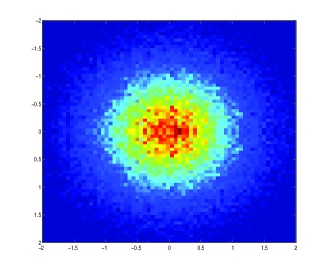
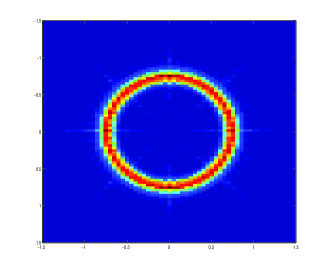
Figure 1. Eigenvalues of $100$ realizations of $n^{-1/2}A_{k,n}$ with $a_{l}\sim N(0,1)$ when (i) $k=1,n=901$ (left) and (ii) $k=2,n=901$ (right). The color represents the height of the histogram - from red (high) to blue (low).

Theorem 1.

Suppose $\{a_{l}\}_{l\geq 0}$ is an i.i.d. sequence of $N(0,1)$ random variables. Let $k\geq 2$ be such that $k=n^{o(1)}$ and $n\to\infty$ with $\gcd(n,k)=1$. Then $F_{n^{-1/2}A_{k,n}}$ converges weakly in probability to the uniform distribution over the circle with center at $(0,0)$ and radius $r=\exp(\mathbb{E}[\log\sqrt{E}])$, $E$ being an exponential random variable with mean one.

Remark 1.

Since $-\log E$ has the standard Gumbel distribution which has mean $\gamma$ where $\gamma\approx 0.57721$ is the Euler-Mascheroni constant, it follows that $r=e^{-\gamma/2}\approx 0.74930$.

In view of Theorem 1, it is natural to consider the case when $k^{g}=\Omega(n)$ and $\gcd(k,n)=1$ where $g$ is a fixed integer. In the next two theorems, we consider two special cases of the above scenario, namely when $n$ divides $k^{g}\pm 1$. Consider the following assumption.

Assumption I. The sequence $\{a_{l}\}_{l\geq 0}$ is independent with mean zero, variance one and for some $\delta>0$,

$$\sup_{n}n^{-1}\sum_{i=0}^{n-1}E|a_{l}|^{2+\delta}<\infty.$$

We are now ready to state our main theorems on the existence of LSD.

Theorem 2.

Suppose $\{a_{l}\}_{l\geq 0}$ satisfies Assumption I. Fix $g\geq 1$ and let $p_{1}$ be the smallest prime divisor of $g$. Suppose $k^{g}=-1+sn$ where $s=1$ if $g=1$ and $s=o(n^{p_{1}-1})$ if $g>1$. Then $F_{n^{-1/2}A_{k,n}}$ converges weakly in probability to $U_{1}(\prod_{j=1}^{g}E_{j})^{1/2g}$ as $n\to\infty$ where $\{E_{j}\}_{1\leq j\leq g}$ are i.i.d. exponentials with mean one and $U_{1}$ is uniformly distributed over the $(2g)$th roots of unity, independent of $\{E_{j}\}_{1\leq j\leq g}$.

Theorem 3.

Suppose $\{a_{l}\}_{l\geq 0}$ satisfies Assumption I. Fix $g\geq 1$ and let $p_{1}$ be the smallest prime divisor of $g$. Suppose $k^{g}=1+sn$ where $s=0$ if $g=1$ and $s=o(n^{p_{1}-1})$ if $g>1$. Then $F_{n^{-1/2}A_{k,n}}$ converges weakly in probability to $U_{2}(\prod_{j=1}^{g}E_{j})^{1/2g}$ as $n\to\infty$ where $\{E_{j}\}_{1\leq j\leq g}$ are i.i.d. exponentials with mean one and $U_{2}$ is uniformly distributed over the unit circle in $\mathbb{R}^{2}$, independent of $\{E_{j}\}_{1\leq j\leq g}$.

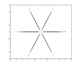
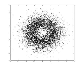
Figure 2. Eigenvalues of $20$ realizations of $n^{-1/2}A_{k,n}$ with $a_{l}\sim\text{Exp}(1)-1$ when (i) $k=11,k^{3}=-1+2n$ (left) and (ii) $k=11,k^{3}=1+2n$ (right).

Remark 2.

(1) Theorem 2 and Theorem 3 recover the LSDs of $k$-circulants for $k=n-1$ and $k=1$ respectively.

(2) While the radial coordinates of the LSD described in Theorem 2 and 3 are same, their angular coordinates differ. While one puts its mass only at discrete places $e^{i2\pi j/2g},1\leq j\leq 2g$ on the unit circle, the other spreads its mass uniformly over the entire unit circle. See Figure 2.

(3) The restriction on $s=(k^{g}\pm 1)/n$ in the above two theorems seems to be a natural one. Suppose $g$ is a prime and so $g=p_{1}$. In this case if $s\geq n^{p_{1}-1}$, then $k$ becomes greater than or equal to $n$ violating the assumption that $k<n$.

(4) We cannot expect similar LSDs to hold for more general cases like $k^{g}=\pm r+n,r>1$ fixed. Compare Figure 2 and Figure 3.

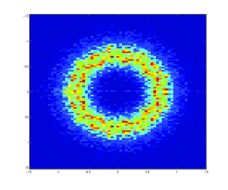
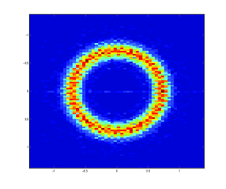
Figure 3. Eigenvalues of $100$ realizations of $n^{-1/2}A_{k,n}$ with $a_{l}\sim N(0,1)$ when (i) $k=16,n=-3+k^{2}$ (left) and (ii) $k=16,n=3+k^{2}$ (right). The color represents the height of the histogram - from red (high) to blue (low).

1.2.2. Spectral radius

For the $k$-circulant, first suppose that the input sequence is i.i.d. standard normal. When $k=1$, it is easy to check that the modulus square of the eigenvalues are exponentials and they are independent of each other. Hence, the appropriately scaled and normalized spectral radius converges to the Gumbel distribution. But when the input sequence is i.i.d. but not necessary normal, that independence structure is lost. A careful use of Komlós-Major-Tusándi type sharp normal approximation results are needed to deal with this case. See Davis and Mikosch (1999)[10]. These approximations imply that the limit continues to be Gumbel. The spectral radius of the $(n-1)$-circulant is the same as that of the circulant and hence it has the same limit. See also Bryc and Sethuraman (2009)[8] who use the same approach for the symmetric circulant.

Now let $g=2$ and for further simplicity, assume that $n=k^{2}+1$. If the input sequence is i.i.d. standard normal, then the modulus of the nonzero eigenvalues are independent and distributed according to $(E_{1}E_{2})^{1/4}$, where $E_{j},j=1,2$ are i.i.d. standard exponential. Thus, the behavior of the spectral radius is the same as that of the maxima of i.i.d variables each distributed as $(E_{1}E_{2})^{1/4}$. This is governed by the tail behaviour of $E_{1}E_{2}$. We deduce this tail behaviour via properties of Bessel functions and the limit again turns out to be Gumbel. Now, as suggested by the results of Davis and Mikosch (1999)[10], even when the input sequence is only assumed to be i.i.d. and not necessarily normal, with suitable moment condition, some kind of invariance principle holds and the same limit persists. We show that this is indeed the case.

Theorem 4.

Suppose $\{a_{l}\}_{l\geq 0}$ is an i.i.d. sequence of random variables with mean zero and variance $1$ and $\mathbb{E}|a_{l}|^{\gamma}<\infty$ for some $\gamma>2$. If $n=k^{2}+1$ then

$$\frac{\texttt{sp}(n^{-1/2}A_{k,n})-d_{q}}{c_{q}}$$

converges in distribution to the standard Gumbel as $n\to\infty$ where $q=q(n)={\lfloor\frac{n}{4}\rfloor}$ and the normalizing constants $c_{n}$ and $d_{n}$ can be taken as follows

(1) $$c_{n}=(8\log n)^{-1/2}\ \ \text{and}\ \ d_{n}=\frac{(\log n)^{1/2}}{\sqrt{2}}\left(1+\frac{1}{4}\frac{\log\log n}{\log n}\right)+\frac{1}{2(8\log n)^{1/2}}\log\frac{\pi}{2}.$$

In the next section we state the basic eigenvalue formula for $k$-circulant and develop some essential properties of the eigenvalues. In Section 3 and Section 4 we state and prove the results on LSD and the spectral radius respectively. An Appendix reproves the known eigenvalue formula for $k$-circulant.

2. Eigenvalues of the $k$-circulant

We first describe the eigenvalues of a $k$-circulant and prove some related auxiliary properties. The formula solution, in particular is already known, see for example Zhou (1996)[32]. We provide a more detailed analysis which we later use in our study of the LSD and the spectral radius. Let

(2) $$\omega=\omega_{n}:=\cos(2\pi/n)+i\sin(2\pi/n),\ i^{2}=-1\ \ \text{and}\ \ \lambda_{t}=\sum\limits_{l=0}^{n-1}a_{l}\omega^{tl},\ \ 0\leq t<n.$$

Remark 3.

Note that $\{\lambda_{t},0\leq t<n\}$ are eigenvalues of the usual circulant matrix $A_{1,n}$.

Let $p_{1}<p_{2}<\cdots<p_{c}$ be all the common prime factors of $n$ and $k$. Then we may write,

(3) $$n=n^{\prime}\prod_{q=1}^{c}p_{q}^{\beta_{q}}\ \text{ and }\ \ k=k^{\prime}\prod_{q=1}^{c}p_{q}^{\alpha_{q}}.$$

Here $\alpha_{q},\ \beta_{q}\geq 1$ and $n^{\prime}$, $k^{\prime}$, $p_{q}$ are pairwise relatively prime. We will show that $(n-n^{\prime})$ eigenvalues of $A_{k,n}$ are zero and $n^{\prime}$ eigenvalues are non-zero functions of $\underline{a}$.

To identify the non-zero eigenvalues of $A_{k,n}$, we need some preparation. For any positive integer $m$, the set $\mathbb{Z}_{m}$ has its usual meaning, that is, $\mathbb{Z}_{m}=\{0,1,2,\ldots,m-1\}.$ We introduce the following family of sets

(4) $$S(x):=\big{\{}xk^{b}\text{ mod }n^{\prime}:b\geq 0\big{\}},\quad x\in\mathbb{Z}_{n^{\prime}}.$$

We observe the following facts about the family of sets $\{S(x)\}_{x\in\mathbb{Z}_{n^{\prime}}}$.

(I) Let $g_{x}=\#S(x)$. We call $g_{x}$ the order of $x$. Note that $g_{0}=1$. It is easy to see that

$$S(x)=\{xk^{b}\text{ mod }n^{\prime}:0\leq b<g_{x}\}.$$

An alternative description of $g_{x}$, which we will use later extensively, is the following. For $x\in\mathbb{Z}_{n^{\prime}}$, let

$$\mathcal{O}_{x}=\{b>0\ :b\text{ is an integer and }xk^{b}=x\text{ mod }n^{\prime}\}.$$

Then $g_{x}=\min O_{x}$, that is, $g_{x}$ is the smallest positive integer $b$ such that $xk^{b}=x\text{ mod }n^{\prime}$.

(II) The distinct sets from the collection $\{S(x)\}_{x\in\mathbb{Z}_{n^{\prime}}}$ forms a partition of $\mathbb{Z}_{n^{\prime}}$. To see this, first note that $x\in S(x)$ and hence $\bigcup_{x\in\mathbb{Z}_{n^{\prime}}}S(x)=\mathbb{Z}_{n^{\prime}}$. Now suppose $S(x)\cap S(y)\neq\emptyset$. Then, $xk^{b_{1}}=yk^{b_{2}}\text{ mod }n^{\prime}$ for some integers $b_{1},b_{2}\geq 1$. Multiplying both sides by $k^{g_{x}-b_{1}}$ we see that, $x\in S(y)$ so that, $S(x)\subseteq S(y)$. Hence, reversing the roles, $S(x)=S(y)$.

We call the distinct sets in $\{S(x)\}_{x\in\mathbb{Z}_{n^{\prime}}}$ the eigenvalue partition of $\mathbb{Z}_{n^{\prime}}$ and denote the partitioning sets and their sizes by

(5) $$\mathcal{P}_{0}=\{0\},\mathcal{P}_{1},\ldots,\mathcal{P}_{\ell-1}\ \ \text{and}\ \ n_{j}=\#\mathcal{P}_{j},\ 0\leq j<\ell.$$

Define

(6) $$\Pi_{j}:=\prod_{t\in\mathcal{P}_{j}}\lambda_{tn/n^{\prime}},\ \ j=0,1,\ldots,\ell-1.$$

The following theorem provides the formula solution for the eigenvalues of $A_{k,n}$. Since this is from a Chinese article which may not be easily accessible to all readers, we have provided a proof in the Appendix.

Theorem 5 (Zhou (1996)[32]).

The characteristic polynomial of $A_{k,n}$ is given by

(7) $$\chiup\left(A_{k,n}\right)(\lambda)=\lambda^{n-n^{\prime}}\prod_{j=0}^{\ell-1}\left(\lambda^{n_{j}}-\Pi_{j}\right).$$

2.1. Some properties of the eigenvalue partition $\{\mathcal{P}_{j},0\leq j<\ell\}$

We collect some simple but useful properties about the eigenvalue partition in the following lemma.

Lemma 1.

(i) Let $x,y\in\mathbb{Z}_{n^{\prime}}$. If $n^{\prime}-t_{0}\in S(y)$  for some $t_{0}\in S(x)$, then for every $t\in S(x)$, we have $n^{\prime}-t\in S(y)$.

(ii) Fix $x\in\mathbb{Z}_{n^{\prime}}$. Then $g_{x}$ divides $g$ for every $g\in\mathcal{O}_{x}$. Furthermore, $g_{1}$ divides $g_{x}$ for each $x\in\mathbb{Z}_{n^{\prime}}$.

(iii) Suppose $g$ divides $g_{1}$. Set $m:=\gcd(k^{g}-1,n^{\prime})$. Let $X(g)$ and $Y(g)$ be defined as

(8) $$X(g):=\Big{\{}x:x\in\mathbb{Z}_{n^{\prime}}\ \ \text{and}\ \ x\ \ \text{has order}\ \ g\Big{\}},\ \ Y(g):=\Big{\{}bn^{\prime}/m\ :\ 0\leq b<m\Big{\}}.$$

Then

$$X(g)\subseteq Y(g),\ \ \#Y(g)=m\ \ \text{and}\ \ \bigcup_{h:h|g}X(h)=Y(g).$$

Proof.

(i) Since $t\in S(x)=S(t_{0})$, we can write $t=t_{0}k^{b}\text{ mod }n^{\prime}$ for some $b\geq 0$. Therefore, $n^{\prime}-t=(n^{\prime}-t_{0})k^{b}\text{ mod }n^{\prime}\in S(n^{\prime}-t_{0})=S(y)$.

(ii) Fix $g\in\mathcal{O}_{x}$. Since $g_{x}$ is the smallest element of $\mathcal{O}_{x}$, it follows that $g_{x}\leq g$. Suppose, if possible, $g=qg_{x}+r$ where $0<r<g_{x}$. By the fact $xg_{x}=x\text{ mod }n^{\prime}$, it then follows that

$$x=xk^{g}\text{ mod }n^{\prime}=xk^{qg_{x}+r}\text{ mod }n^{\prime}=xk^{r}\text{ mod }n^{\prime}.$$

This implies that $r\in\mathcal{O}_{x}$ and $r<g_{x}$ which is a contradiction to the fact that $g_{x}$ is the smallest element in $\mathcal{O}_{x}$. Hence, we must have $r=0$ proving that $g$ divides $g_{1}$.

Note that $k^{g_{1}}=1\text{ mod }n^{\prime}$, implying that $xk^{g_{1}}=x\text{ mod }n^{\prime}$. Therefore $g_{1}\in\mathcal{O}_{x}$ proving the assertion.

(iii) Clearly, $\#Y(g)=m$. Fix $x\in X(h)$ where $h$ divides $g$. Then, $xk^{g}=x(k^{h})^{g/h}=x\mbox{ mod }n^{\prime}$, since $g/h$ is a positive integer. Therefore $n^{\prime}$ divides $x(k^{g}-1)$. So, $n^{\prime}/m$ divides $x(k^{g}-1)/m$. But $n^{\prime}/m$ is relatively prime to $(k^{g}-1)/m$ and hence $n^{\prime}/m$ divides $x$. So, $x=bn^{\prime}/m$ for some integer $b\geq 0$. Since $0\leq x<n^{\prime}$, we have $0\leq b<m$, and $x\in Y(g)$, proving $\bigcup_{h:h|g}X(h)\subseteq Y(g)$ and in particular, $X(g)\subseteq Y(g)$.

On the other hand, take $0\leq b<g$. Then $\left(bn^{\prime}/m\right)k^{g}=\left(bn^{\prime}/m\right)\text{ mod }n^{\prime}$. Hence, $g\in\mathcal{O}_{bn^{\prime}/m}$ which implies, by part (ii) of the lemma, that $g_{cn^{\prime}/m}$ divides $g$. Therefore, $Y(g)\subseteq\bigcup_{h:h|g}X(h)$ which completes the proof. $\Box$ ∎

Lemma 2.

Let $g_{1}=q_{1}^{\gamma_{1}}q_{2}^{\gamma_{2}}\ldots q_{m}^{\gamma_{m}}$ where $q_{1}<q_{2}<\ldots<q_{m}$ are primes. Define for $1\leq j\leq m$,

$$L_{j}:=\left\{q_{i_{1}}q_{i_{2}}\cdots q_{i_{j}}:1\leq i_{1}<\ldots<i_{j}\leq m\right\}$$

and

$$G_{j}=\sum\limits_{l_{j}\in L_{j}}\#Y(g_{1}/\ell_{j})=\sum\limits_{l_{j}\in L_{j}}\gcd\left(k^{g_{1}/\ell_{j}}-1,n^{\prime}\right).$$

Then we have

(i) $\#\left\{x\in\mathbb{Z}_{n^{\prime}}:g_{x}<g_{1}\right\}=G_{1}-G_{2}+G_{3}-G_{4}+\cdots$.

(ii) $G_{1}-G_{2}+G_{3}-G_{4}+\cdots\leq G_{1}.$

Proof.

Fix $x\in\mathbb{Z}_{n^{\prime}}$. By Lemma 1(ii), $g_{x}$ divides $g_{1}$ and hence we can write $g_{x}=q_{1}^{\eta_{1}}\ldots q_{m}^{\eta_{m}}$ where, $0\leq\eta_{b}\leq\gamma_{b}$ for $1\leq b\leq m$. Since $g_{x}<g_{1}$, there is at least one $b$ so that $\eta_{b}<\gamma_{b}$. Suppose that exactly $h$-many $\eta$’s are equal to the corresponding $\gamma$’s where $0\leq h<m$. To keep notation simple, we will assume that, $\eta_{b}=\gamma_{b},\ 1\leq b\leq h$ and $\eta_{b}<\gamma_{b},\ h+1\leq b\leq m$.

(i) Then $x\in Y(g_{1}/q_{b})$ for $h+1\leq b\leq m$ and $x\not\in Y(g_{1}/q_{b})$ for $1\leq b\leq h$. So, $x$ is counted $(m-h)$ times in $G_{1}$. Similarly, $x$ is counted ${m-h\choose 2}$ times in $G_{2}$, ${m-h\choose 3}$ times in $G_{3}$, and so on. Hence, total number of times $x$ is counted in $(G_{1}-G_{2}+G_{3}-\ldots)$ is

$${m-h\choose 1}-{m-h\choose 2}+{m-h\choose 3}-\ldots=1.$$

(ii) Note that $m-h\geq 1$. Further, each element in the set $\left\{x\in\mathbb{Z}_{n^{\prime}}:g_{x}<g_{1}\right\}$ is counted once in $G_{1}-G_{2}+G_{3}-\ldots$ and $(m-h)$ times in $G_{1}$. The result follows immediately. ∎

2.2. Asymptotic negligibility of lower order elements

We will now consider the elements in $\mathbb{Z}_{n{\prime}}$ with order less than that of $1\in\mathbb{Z}_{n{\prime}}$ which has the highest order $g_{1}$. We will need the proportion of such elements in $\mathbb{Z}_{n{\prime}}$. So, we define

(9) $$\upsilon_{k,n^{\prime}}:=\frac{1}{n^{\prime}}\#\{x\in\mathbb{Z}_{n{\prime}}:g_{x}<g_{1}\}.$$

To derive the LSD in the special cases we have in mind, the asymptotic negligibility of $\upsilon_{k,n^{\prime}}$ turns out to be important. The following two lemmas establish upper bounds on $\upsilon_{k,n^{\prime}}$ and will be crucially used later.

Lemma 3.

(i) If $g_{1}=2$, then $\displaystyle\upsilon_{k,n^{\prime}}=\gcd(k-1,n^{\prime})/n^{\prime}$.

(ii) If $g_{1}\geq 4$ is even, and $k^{g_{1}/2}=-1\mbox{ mod }n$, then $\displaystyle\upsilon_{k,n^{\prime}}\leq 1+\sum_{b|g_{1},\ b\geq 3}\gcd(k^{g_{1}/b}-1,n^{\prime}).$

(iii) If $g_{1}\geq 2$ and $q_{1}$ is the smallest prime divisor of $g_{1}$, then $\displaystyle\upsilon_{k,n^{\prime}}<2{n^{\prime}}^{-1}k^{g_{1}/q_{1}}.$

Proof.

Part (i) is immediate from Lemma 2 which asserts that $n^{\prime}\upsilon_{k,n^{\prime}}=\#Y(1)=\gcd(k-1,n^{\prime})$.

(ii) Fix $x\in\mathbb{Z}_{n^{\prime}}$ with $g_{x}<g_{1}$. Since $g_{x}$ divides $g_{1}$ and $g_{x}<g_{1}$, $g_{x}$ must be of the form $g_{1}/b$ for some integer $b\geq 2$ provided $g_{1}/b$ is an integer. If $b=2$, then $xk^{g_{1}/2}=xk^{g_{x}}=x\text{ mod }n^{\prime}$. But $k^{g_{1}/2}=-1\mbox{ mod }n^{\prime}$ and so, $xk^{g_{1}/2}=-x\mbox{ mod }n^{\prime}$. Therefore, $2x=0\mbox{ mod }n^{\prime}$ and $x$ can be either $0$ or $n^{\prime}/2$, provided, of course, $n^{\prime}/2$ is an integer. But $g_{0}=1<2\leq g_{1}/2$ so $x$ cannot be $0$. So, there is at most one element in the set $X(g_{1}/2)$. Thus we have,

$$\#\{x\in\mathbb{Z}_{n^{\prime}}:g_{x}<g_{1}\} =\#X(g_{1}/2)+\sum_{b|g_{1},\ b\geq 3}\#\{x\in\mathbb{Z}_{n^{\prime}}:g_{x}=g_{1}/b\}$$

$$=\#X(g_{1}/2)+\sum_{b|g_{1},\ b\geq 3}\#X(g_{1}/b)$$

$$\leq 1+\sum_{b|g_{1},\ b\geq 3}\#Y(g_{1}/b)\quad[\text{by Lemma \ref{lem:partitionproperties}(iii)}]$$

$$=1+\sum_{b|g_{1},\ b\geq 3}\gcd(k^{g_{1}/b}-1,n^{\prime})\quad[\text{by Lemma \ref{lem:partitionproperties}(iii)}.]$$

(iii) As in Lemma 2, let $g_{1}=q_{1}^{\gamma_{1}}q_{2}^{\gamma_{2}}\ldots q_{m}^{\gamma_{m}}$ where $q_{1}<q_{2}<\ldots<q_{m}$ are primes. Then by Lemma 2,

$$n^{\prime}\times\upsilon_{k,n^{\prime}}=G_{1}-G_{2}+G_{3}-G_{4}+\ldots\leq G_{1} =\sum\limits_{b=1}^{m}\gcd(k^{g_{1}/q_{b}}-1,n^{\prime})$$

$$<\sum\limits_{b=1}^{m}k^{g_{1}/q_{b}}\leq 2k^{g_{1}/q_{1}}$$

where the last inequality follows from the observation

$$\sum\limits_{b=1}^{m}k^{g_{1}/q_{b}}\leq k^{g_{1}/q_{1}}\sum\limits_{b=1}^{m}k^{-g_{1}(q_{b}-q_{1})/q_{1}q_{b}}\leq k^{g_{1}/q_{1}}\sum\limits_{b=1}^{m}k^{-(q_{b}-q_{1})}\leq k^{g_{1}/q_{1}}\sum\limits_{b=1}^{m}k^{-(b-1)}\leq 2k^{g_{1}/q_{1}}.$$

∎

Lemma 4.

Let $b$ and $c$ be two fixed positive integers. Then for any integer $k\geq 2$, the following inequality holds in each of the four cases,

$$\gcd(k^{b}\pm 1,k^{c}\pm 1)\leq k^{\gcd(b,c)}+1.$$

Proof.

The assertion trivially follows if one of $b$ and $c$ divides other. So, we assume, without loss, that $b<c$ and $b$ does not divide $c$. Since, $k^{c}\pm 1=k^{c-b}(k^{b}+1)+(-k^{c-b}\pm 1)$, we can write

$$\gcd(k^{b}+1,k^{c}\pm 1)=\gcd(k^{b}+1,k^{c-b}\mp 1).$$

Similarly,

$$\gcd(k^{b}-1,k^{c}\pm 1)=\gcd(k^{b}-1,k^{c-b}\pm 1).$$

Moreover, if we write $c_{1}=c-\lfloor c/b\rfloor b$, then by repeating the above step $\lfloor c/b\rfloor$ times, we can see that $\gcd(k^{b}\pm 1,k^{c}\pm 1)$ is equal to one of $\gcd(k^{b}\pm 1,k^{c_{1}}\pm 1)$. Now if $c_{1}$ divides $b$, then $\gcd(b,c)=c_{1}$ and we are done. Otherwise, we can now repeat the whole argument with $b=c_{1}$ and $c=b$ to deduce that $\gcd(k^{b}\pm 1,k^{c_{1}}\pm 1)$ is one of $\gcd(k^{b_{1}}\pm 1,k^{c_{1}}\pm 1)$ where $b_{1}=b-\lfloor b/c_{1}\rfloor c_{1}$. We continue in the similar fashion by reducing each time one of the two exponents of $k$ in the gcd and the lemma follows once we recall Euclid’s recursive algorithm for computing the gcd of two numbers. ∎

Lemma 5.

(i) Fix $g\geq 1$. Suppose $k^{g}=-1+sn$, $n\to\infty$ with $s=1$ if $g=1$ and $s=o(n^{p_{1}-1})$ if $g>1$ where $p_{1}$ is the smallest prime divisor of $g$. Then $g_{1}=2g$ for all but finitely many $n$ and $\upsilon_{k,n}\to 0.$

(ii) Suppose $k^{g}=1+sn$, $g\geq 1$ fixed, $n\to\infty$ with $s=0$ if $g=1$ and $s=o(n^{p_{1}-1})$ where $p_{1}$ is the smallest prime divisor of $g$. Then $g_{1}=g$ for all but finitely many $n$ and $\upsilon_{k,n}\to 0.$

Proof.

(i) First note that $\gcd(n,k)=1$ and therefore $n^{\prime}=n$. When $g=1$, it is easy to check that $g_{1}$ =2 and by Lemma 3(i), $\upsilon_{k,n}\leq 2/n$.

Now assume $g>1$. Since $k^{2g}=(sn-1)^{2}=1\text{ mod }n$, $g_{1}$ divides $2g$. Observe that $g_{1}\neq g=2g/2$ because $k^{g}=-1\text{ mod }n$.

If $g_{1}=2g/b$, where $b$ divides $g$ and $b\geq 3$, then by Lemma 4,

$$\gcd(k^{g_{1}}-1,n)=\gcd\big{(}k^{2g/b}-1,(k^{g}+1)/s\big{)}\leq\gcd\big{(}k^{2g/b}-1,k^{g}+1\big{)}\leq k^{\gcd(2g/b,\ g)}+1.$$

Note that since $\gcd(2g/b,g)$ divides $g$ and $\gcd(2g/b,g)\leq 2g/b<g$, we have $\gcd(2g/b,g)\leq g/p_{1}$. Consequently,

(10) $$\gcd(k^{2g/b}-1,n)\leq k^{g/p_{1}}+1\leq(sn-1)^{1/p_{1}}+1=o(n),$$

which is a contradiction to the fact that $k^{g_{1}}=1\text{ mod }n$ which implies that $\gcd(k^{g_{1}}-1,n)=n$. Hence, $g_{1}=2g$. Now by Lemma 3(ii) it is enough to show that for any fixed $b\geq 3$ so that $b$ divides $g_{1}$,

$$\gcd(k^{g_{1}/b}-1,n)/n=o(1)\ \ \text{as}\ \ n\to\infty,$$

which we have already proved in (10).

(ii) Again $\gcd(n,k)=1$ and $n^{\prime}=n$. The case when $g=1$ is trivial as then we have $g_{x}=1$ for all $x\in\mathbb{Z}_{n}$ and $\upsilon_{k,n}=0$.

Since $k^{g}=1\text{ mod }n$, $g_{1}$ divides $g$. If $g_{1}<g$, then $g_{1}\leq g/p_{1}$ which implies that $k^{g_{1}}\leq k^{g/p_{1}}=(sn+1)^{1/p_{1}}=o(n)$, which is a contradiction. Thus, $g=g_{1}$.

Now Lemma 3(iii) immediately yields,

$$\upsilon_{k,n}<\frac{2k^{g_{1}/p_{1}}}{n}\leq\frac{2(1+sn)^{1/p_{1}}}{n}=o(1).$$

∎

3. Proof of Theorem 1, Theorem 2 and Theorem 3

3.1. Properties of eigenvalues of Gaussian circulant matrices

Suppose $\{a_{l}\}_{l\geq 0}$ are independent, mean zero and variance one random variables. Fix $n$. For $1\leq t<n$, let us split $\lambda_{t}$ into real and complex parts as $\lambda_{t}=a_{t,n}+ib_{t,n}$, that is,

(11) $$a_{t,n}=\sum\limits_{l=0}^{n-1}a_{l}\cos\left(\frac{2\pi tl}{n}\right),\ \ b_{t,n}=\sum\limits_{l=0}^{n-1}a_{l}\sin\left(\frac{2\pi tl}{n}\right).$$

(12) $$\sum_{l=0}^{n-1}\cos\left(\frac{2\pi tl}{n}\right)\sin\left(\frac{2\pi t^{\prime}l}{n}\right)=0,\ \forall t,t^{\prime} \text{ and }\ \sum_{l=0}^{n-1}\cos^{2}\left(\frac{2\pi tl}{n}\right)=\sum_{l=0}^{n-1}\sin^{2}\left(\frac{2\pi tl}{n}\right)=n/2\quad\forall 0<t<n.$$

(13) $$\sum_{l=0}^{n-1}\cos\left(\frac{2\pi tl}{n}\right)\cos\left(\frac{2\pi t^{\prime}l}{n}\right)=0,\ \text{ and }\sum_{l=0}^{n-1}\sin\left(\frac{2\pi tl}{n}\right)\sin\left(\frac{2\pi t^{\prime}l}{n}\right)=0\quad\forall t\neq t^{\prime}\ \ (\text{ mod }n).$$

For $z\in\mathbb{C}$, by $\bar{z}$ we mean, as usual, the complex conjugate of $z$. For all $0<t,t^{\prime}<n$, the following identities can easily be verified using the above orthogonality relations

$$\mathbb{E}(a_{t,n}b_{t,n})=0,\ \ \text{and}\ \ \mathbb{E}(a_{t,n}^{2})=\mathbb{E}(b_{t,n}^{2})=n/2,$$

$$\bar{\lambda}_{t}=\lambda_{n-t},\ \ \mathbb{E}(\lambda_{t}\lambda_{t^{\prime}})=n\mathbb{I}(t+t^{\prime}=n),\ \ \mathbb{E}(|\lambda_{t}|^{2})=n.$$

The following Lemma will be used in the proof of Theorem 2 and Theorem 3.

Lemma 6.

Fix $k$ and $n$. Suppose that $\{a_{l}\}_{0\leq l<n}$ are i.i.d. standard normal random variables. Recall the notations $\mathcal{P}_{j}$ and $\Pi_{j}$ from Section 2. Then

(a) For every $n$, $n^{-1/2}a_{t,n},n^{-1/2}b_{t,n}$, $0\leq t\leq n/2$ are i.i.d. normal with mean zero and variance $1/2$. Consequently, any subcollection $\{\Pi_{j_{1}},\Pi_{j_{2}},\ldots\}$ of $\{\Pi_{j}\}_{0\leq j<\ell}$, so that no member of the corresponding partition blocks $\{\mathcal{P}_{j_{1}},\mathcal{P}_{j_{2}},\ldots\}$ is a conjugate of any other, are mutually independent.

(b) Suppose $1\leq j<\ell$ and $\mathcal{P}_{j}\cap(n-\mathcal{P}_{j})=\emptyset$. Then all $n^{-n_{j}/2}\Pi_{j}$ are distributed as $n_{j}$-fold product of i.i.d. random variables, each of which is distributed as $E^{1/2}U$ where $E$ and $U$ are independent random variables, $E$ is exponential with mean one and $U$ is uniform over the unit circle in $\mathbb{R}^{2}$.

(c) Suppose $1\leq j<\ell$ and $\mathcal{P}_{j}=n-\mathcal{P}_{j}$ and $n/2\not\in\mathcal{P}_{j}$. Then $n^{-n_{j}/2}\Pi_{j}$ are distributed as $(n_{j}/2)$-fold product of i.i.d. exponential random variables with mean one.

Proof.

(a) Being linear combinations of $\{a_{l}\}_{0\leq l<n}$, $n^{-1/2}a_{t,n},n^{-1/2}b_{t,n}$, $0\leq t\leq n/2$ are all jointly Gaussian. By (12), they have mean zero, variance $1/2$ and are independent.

(b) By part (a) of the lemma, note that $n^{-1/2}\lambda_{t}=n^{-1/2}a_{t,n}+in^{-1/2}b_{t,n}$ is a complex normal random variable with mean zero and variance $1/2$ for every $0<t<n$ and moreover, they are independent by the given restriction on $\mathcal{P}_{j}$. The assertion follows by the observation that such a complex normal is same as $E^{1/2}U$ in distribution.

(c) If $t\in\mathcal{P}_{j}$ then $n-t\in\mathcal{P}_{j}$ too and $t\neq n-t$. Thus $n^{-1}\lambda_{t}\lambda_{n-t}=n^{-1}(a_{t,n}^{2}+b^{2}_{t,n})$ which, by part (a), is distributed as $Y/2$ where $Y$ is Chi-square with two degrees of freedom. Note that $Y/2$ has the same distribution as that of exponential random variable with mean one. The proof is complete once we observe that $n_{j}$ is necessarily even and the $\lambda_{t}$’s associated with $\mathcal{P}_{j}$ can be grouped into $n_{j}/2$ disjoint pairs like above which are mutually independent. ∎

3.2. Proof of Theorem 1

Recall the notation $\lambda_{j},\ell,\mathcal{P}_{j},n_{j}$ and $g_{x}$ from Section 2. By Theorem 5, the eigenvalues of $n^{-1/2}A_{k,n}$ are given by

$$\exp\Big{(}\frac{2\pi is}{n_{j}}\Big{)}\times\Big{(}\prod_{t\in\mathcal{P}_{j}}|n^{-1/2}\lambda_{t}|\Big{)}^{1/n_{j}},1\leq s\leq n_{j},\ 0\leq j<\ell,$$

where $i=\sqrt{-1}$. Fix any $\varepsilon>0$ and $0<\theta_{1}<\theta_{2}<2\pi$. Define

$$B(\theta_{1},\theta_{2},\varepsilon)=\Big{\{}(x,y)\in\mathbb{R}^{2}:r-\varepsilon<\sqrt{x^{2}+y^{2}}<r+\varepsilon,\tan^{-1}(y/x)\in[\theta_{1},\theta_{2}]\Big{\}}.$$

Clearly, it is enough to prove that as $n\to\infty$,

(14) $$\frac{1}{n}\sum_{j=0}^{\ell-1}\sum_{s=1}^{n_{j}}\mathbb{I}\left(\exp\Big{(}\frac{2\pi is}{n_{j}}\Big{)}\times\Big{(}\prod_{t\in\mathcal{P}_{j}}|n^{-1/2}\lambda_{t}|\Big{)}^{1/n_{j}}\in B(\theta_{1},\theta_{2},\varepsilon)\right)\stackrel{{\scriptstyle P}}{{\to}}\frac{(\theta_{2}-\theta_{1})}{2\pi}.$$

Note that for a fixed positive integer $C$, we have

$$n^{-1}\sum_{1\leq j<\ell:n_{j}\leq C}n_{j} \leq n^{-1}\sum_{u=2}^{C}\#\big{\{}1\leq x<n:g_{x}=u\big{\}}$$

$$\leq n^{-1}\sum_{u=2}^{C}\#\big{\{}1\leq x<n:xk^{u}=x\mbox{ mod }n\big{\}}$$

$$=n^{-1}\sum_{u=2}^{C}\#\big{\{}1\leq x<n:x(k^{u}-1)=sn\text{ for some }s\geq 1\big{\}}$$

$$\leq n^{-1}\sum_{u=2}^{C}(k^{u}-1)\leq n^{-1}Ck^{C}\to 0,\text{as}\ \ n\to\infty.$$

Therefore, if we define

$$N_{C}=\sum_{j=0:\ n_{j}\leq C}^{\ell-1}n_{j},$$

then the above result combined with the fact that $\mathcal{P}_{0}=\{0\}$ yields $N_{C}/n\to 0$. With $C>(2\pi)/(\theta_{2}-\theta_{1})$, the left side of (14) can rewritten as

$$\frac{1}{n}\sum_{j=0}^{\ell-1}\#\left\{s:\frac{2\pi s}{n_{j}}\in[\theta_{1},\theta_{2}],s=1,2,\ldots,n_{j}\right\}\times\mathbb{I}\left(\Big{(}\prod_{t\in\mathcal{P}_{j}}|n^{-1/2}\lambda_{t}|\Big{)}^{1/n_{j}}\in(r-\varepsilon,r+\varepsilon)\right)$$

$$= \frac{n-N_{C}}{n}\frac{1}{n-N_{C}}\sum_{j=0,\ n_{j}>C}^{\ell-1}n_{j}\times n_{j}^{-1}\#\left\{s:\frac{s}{n_{j}}\in(2\pi)^{-1}[\theta_{1},\theta_{2}],s=1,\ldots,n_{j}\right\}$$

$$\hskip 113.81102pt\times\mathbb{I}\left(\Big{(}\prod_{t\in\mathcal{P}_{j}}|n^{-1/2}\lambda_{t}|\Big{)}^{1/n_{j}}\in(r-\varepsilon,r+\varepsilon)\right)+O\left(\frac{N_{C}}{n}\right)$$

$$= \frac{1}{n-N_{C}}\sum_{j=0,\ n_{j}>C}^{\ell-1}n_{j}\times\left(\frac{(\theta_{2}-\theta_{1})}{2\pi}+O(C^{-1})\right)\times\mathbb{I}\left(\Big{(}\prod_{t\in\mathcal{P}_{j}}|n^{-1/2}\lambda_{t}|\Big{)}^{1/n_{j}}\in(r-\varepsilon,r+\varepsilon)\right)+O\left(\frac{N_{C}}{n}\right)$$

$$= \frac{1}{n-N_{C}}\sum_{j=0,\ n_{j}>C}^{\ell-1}n_{j}\times\frac{(\theta_{2}-\theta_{1})}{2\pi}\times\mathbb{I}\left(\Big{(}\prod_{t\in\mathcal{P}_{j}}|n^{-1/2}\lambda_{t}|\Big{)}^{1/n_{j}}\in(r-\varepsilon,r+\varepsilon)\right)+O(C^{-1})+O\left(\frac{N_{C}}{n}\right)$$

(15) $$= \frac{(\theta_{2}-\theta_{1})}{2\pi}+\frac{1}{n-N_{C}}\sum_{j=0,\ n_{j}>C}^{\ell-1}n_{j}\times\mathbb{I}\left(\Big{(}\prod_{t\in\mathcal{P}_{j}}|n^{-1/2}\lambda_{t}|\Big{)}^{1/n_{j}}\not\in(r-\varepsilon,r+\varepsilon)\right)+O(C^{-1})+O\left(\frac{N_{C}}{n}\right).$$

To show that the second term in the above expression converges to zero in $L^{1}$, hence in probability, it remains to prove,

(16) $$\mathbb{P}\left(\Big{(}\prod_{t\in\mathcal{P}_{j}}|n^{-1/2}\lambda_{t}|\Big{)}^{1/n_{j}}\not\in(r-\varepsilon,r+\varepsilon)\right)$$

is uniformly small for all $j$ such that $n_{j}>C$ and for all but finitely many $n$ if we take $C$ sufficiently large.

By Lemma 6, for each $1\leq t<n$, $|n^{-1/2}\lambda_{t}|^{2}$ is an exponential random variable with mean one, and $\lambda_{t}$ is independent of $\lambda_{t^{\prime}}$ if $t^{\prime}\neq n-t$ and $|\lambda_{t}|=|\lambda_{t^{\prime}}|$ otherwise. Let $E,E_{1},E_{2},\ldots$ be i.i.d.  exponential random variables with mean one. Observe that depending or whether or not $\mathcal{P}_{j}$ is conjugate to itself, (16) equals respectively,

$$\mathbb{P}\left(\Big{(}\prod_{t=1}^{n_{j}/2}E_{t}\Big{)}^{1/n_{j}}\not\in(r-\varepsilon,r+\varepsilon)\right)\ \ \text{or}\ \ \mathbb{P}\left(\Big{(}\prod_{t=1}^{n_{j}}\sqrt{E}_{t}\Big{)}^{1/n_{j}}\not\in(r-\varepsilon,r+\varepsilon)\right).$$

The theorem now follows by letting first $n\to\infty$ and then $C\to\infty$ in (3.2) and by observing that Strong Law of Large Numbers implies that

$$\left(\prod_{t=1}^{C}\sqrt{E}_{t}\right)^{1/C}\to r=\exp(\mathbb{E}[\log\sqrt{E}])\quad\text{almost surely, \ \ \ as }C\to\infty.$$

$\square$

3.3. Invariance Principle

For a set $B\subseteq\mathbb{R}^{d},d\geq 1$, let $(\partial B)^{\eta}$ denote the ‘$\eta$-boundary’ of the set $B$, that is, $(\partial B)^{\eta}:=\big{\{}y\in\mathbb{R}^{d}:\|y-z\|\leq\eta\text{ for some }z\in\partial B\big{\}}$. By $\Phi_{d}(\cdot)$ we always mean the probability distribution of a $d$-dimensional standard normal vector. We drop the subscript $1$ and write just $\Phi(\cdot)$ to denote the distribution of a standard normal random variable.

The proof of the following Lemma follows easily from Theorem 18.1, page 181 of Bhattacharya and Ranga Rao (1976)[2]. We omit the proof.

Lemma 7.

Let $X_{1},\ldots,X_{m}$ be $\mathbb{R}^{d}$-valued independent, mean zero random vectors and let $V_{m}={m}^{-1}\sum_{j=1}^{m}\mathrm{Cov}(X_{j})$ be positive-definite. Let $G_{m}$ be the distribution of ${m}^{-1/2}T_{m}(X_{1}+X_{2}+\cdots+X_{m})$, where $T_{m}$ is the symmetric, positive-definite matrix satisfying $T_{m}^{2}=V_{m}^{-1}$. If for some $\delta>0$, $\mathbb{E}\|X_{j}\|^{(2+\delta)}<\infty$ for each $1\leq j\leq m$, then there exist constants $C_{i}=C_{i}(d)$, $i=1,2$ such that for any Borel set $A\subseteq\mathbb{R}^{d}$,

$$|G_{m}(A)-\Phi_{d}(A)| \leq C_{1}m^{-\delta/2}\Big{(}m^{-1}\sum_{j=1}^{m}\mathbb{E}\|T_{m}X_{j}\|^{(2+\delta)}\Big{)}+2\sup_{y\in\mathbb{R}^{d}}\Phi_{d}\Big{(}(\partial A)^{\eta}-y\Big{)},$$

$$\leq C_{1}m^{-\delta/2}(\lambda_{\min}(V_{m}))^{-(2+\delta)}\rho_{2+\delta}+2\sup_{y\in\mathbb{R}^{d}}\Phi_{d}\Big{(}(\partial A)^{\eta}-y\Big{)},$$

where $\rho_{2+\delta}=m^{-1}\sum_{j=1}^{m}\mathbb{E}\|X_{j}\|^{(2+\delta)}$, $\lambda_{\min}(V_{m})>0$ is the smallest eigenvalue of $V_{m}$, and $\eta=C_{2}\rho_{2+\delta}n^{-\delta/2}$.

3.4. Proof of Theorem 2

Since $\gcd(k,n)=1$, $n^{\prime}=n$ in Theorem 5 and hence there are no zero eigenvalues. By Lemma 5 (i), $\upsilon_{k,n}/n\to 0$ and hence the corresponding eigenvalues do not contribute to the LSD. It remains to consider only the eigenvalues corresponding to the sets $\mathcal{P}_{j}$ of size exactly equal to $g_{1}$. From Lemma 5(i), $g_{1}=2g$ for $n$ sufficiently large.

Recall the quantities $n_{j}=\#\mathcal{P}_{j}$, $\Pi_{j}=\Pi_{t\in\mathcal{P}_{l}}\lambda_{t}$, where $\lambda_{t}=\sum\limits_{l=0}^{n-1}a_{\ell}\omega^{tl}$, $0\leq j<n$. Also, for every integer $t\geq 0$, $tk^{g}=(-1+sn)t=-t\text{ mod }n$, so that, $\lambda_{t}$ and $\lambda_{n-t}$ belong to same partition block $S(t)=S(n-t)$. Thus each $\Pi_{j}$ is a nonnegative real number. Let us define

$$J_{n}=\{0\leq j<\ell:\#\mathcal{P}_{j}=2g\},$$

so that $n=2g\#J_{n}+n\upsilon_{k,n}$. Since, $\upsilon_{k,n}\to 0$, $(\#J_{n})^{-1}n\to 2g$. Without any loss, we denote the index set of such $j$ as $J_{n}=\{1,2,\ldots\#J_{n}\}$.

Let $1,\varrho,\varrho^{2},\ldots\varrho^{2g-1}$ be all the $(2g)$th roots of unity. Since $n_{j}=2g$ for every $j\in J_{n}$, the eigenvalues corresponding to the set $\mathcal{P}_{j}$ are:

$$\Pi_{j}^{1/2g},\Pi_{j}^{1/2g}\varrho,\ldots\Pi_{j}^{1/2g}\varrho^{2g-1}.$$

Hence, it suffices to consider only the empirical distribution of $\Pi_{j}^{1/2g}$ as $j$ varies over the index set $J_{n}$: if this sequence of empirical distributions has a limiting distribution $F$, say, then the LSD of the original sequence $n^{-1/2}A_{k,n}$ will be $(r,\theta)$ in polar coordinates where $r$ is distributed according to $F$ and $\theta$ is distributed uniformly across all the $2g$ roots of unity and $r$ and $\theta$ are independent. With this in mind, and remembering the scaling $\sqrt{n}$, we consider

$$F_{n}(x)=(\#J_{n})^{-1}\sum_{j=1}^{\#J_{n}}\mathbb{I}\left(\left[n^{-g}\Pi_{j}\right]^{\frac{1}{2g}}\leq x\right).$$

Since the set of $\lambda$ values corresponding to any $\mathcal{P}_{j}$ is closed under conjugation, there exists a set $\mathcal{A}_{j}\subset\mathcal{P}_{j}$ of size $g$ such that

$$\mathcal{P}_{j}=\{x:x\in\mathcal{A}_{j}\text{ or }n-x\in\mathcal{A}_{j}\}.$$

Combining each $\lambda_{t}$ with its conjugate, and recalling the definition of $\{a_{t,n}\}$ and $\{b_{t,n}\}$ in (11), we may write $\Pi_{j}$ as

$$\Pi_{j}=\prod_{t\in\mathcal{A}_{j}}(a_{t,n}^{2}+b_{t,n}^{2}).$$

First assume the random variables $\{a_{l}\}_{l\geq 0}$ are i.i.d. standard normal. Then by Lemma 6(c), $F_{n}$ is the usual empirical distribution of $\#J_{n}$ observations on $(\prod_{j=1}^{g}E_{j})^{1/2g}$ where $\{E_{j}\}_{1\leq j\leq g}$ are i.i.d. exponentials with mean one. Thus by Glivenko-Cantelli Lemma, this converges to the distribution of $(\prod_{j=1}^{g}E_{j})^{1/2g}$. Though the variables involved in the empirical distribution form a triangular sequence, the convergence is still almost sure due to the specific bounded nature of the indicator functions involved. This may be proved easily by applying Hoeffding’s inequality and Borel-Cantelli lemma.

As mentioned earlier, all eigenvalues corresponding to any partition block $\mathcal{P}_{j}$ are all the $(2g)$th roots of the product $\Pi_{j}$. Thus, the limit claimed in the statement of the theorem holds. So we have proved the result when the random variables $\{a_{l}\}_{l\geq 0}$ are i.i.d. standard normal.

Now suppose that the variables $\{a_{l}\}_{l\geq 0}$ are not necessarily normal. This case is tackled by normal approximation arguments similar to Bose and Mitra (2002)[5] who deal with the case $k=n-1$ (and hence $g=1$). We now sketch some of the main steps.

The basic idea remains the same but in this general case, a technical complication arises as we need to control the Gaussian measure of the $\eta$-boundaries of some non-convex sets once we apply the invariance lemma (Lemma 7). We overcome this difficulty by suitable compactness argument.

We start by defining

$$F(x)=\mathbb{P}\left(\big{(}\prod_{j=1}^{g}E_{j}\big{)}^{1/2g}\leq x\right),\ \ x\in\mathbb{R}.$$

To show that the ESD converges to the required LSD in probability, we show that for every $x>0$,

$$\mathbb{E}[F_{n}(x)]\rightarrow F(x)\ \ \mbox{and}\ \ \mathrm{Var}[F_{n}(x)]\rightarrow 0.$$

Note that for $x>0$,

$$\mathbb{E}[F_{n}(x)]=(\#J_{n})^{-1}\sum_{j=1}^{\#J_{n}}\mathbb{P}\big{(}n^{-g}\Pi_{j}\leq x^{2g}\big{)}.$$

Lemma 6 motivates using normal approximations. Towards using Lemma 7, define $2g$ dimensional random vectors

$$X_{l,j}=2^{1/2}\left(a_{l}\cos\left(\frac{2\pi tl}{n}\right),\ \ a_{l}\sin\left(\frac{2\pi tl}{n}\right):\ \ t\in\mathcal{A}_{j}\right)\quad 0\leq l<n,1\leq j\leq\#J_{n}.$$

Note that

$$\mathbb{E}(X_{l,j})=0\ \ \text{and}\ \ n^{-1}\sum_{l=1}^{n-1}\text{Cov}(X_{l,j})=I_{2g}\ \ \forall\ \ l,\ j.$$

Fix $x>0$. Define the set $A\subseteq\mathbb{R}^{2g}$ as

$$A:=\Big{\{}(x_{j},y_{j}:1\leq j\leq g):\prod_{j=1}^{g}\big{[}2^{-1}(x_{j}^{2}+y_{j}^{2})\big{]}\leq x^{2g}\Big{\}}.$$

Note that

$$\Big{\{}n^{-g}\Pi_{j}\leq x^{2g}\Big{\}}=\Big{\{}n^{-1/2}\sum_{l=0}^{n-1}X_{l,j}\in A\Big{\}}.$$

We want to prove

$$\mathbb{E}[F_{n}(x)]-\Phi_{2g}(A)=(\#J_{n})^{-1}\sum_{l=1}^{\#J_{n}}\left(\mathbb{P}\big{(}n^{-g}\Pi_{j}\leq x^{2g}\big{)}-\Phi_{2g}(A)\right)\rightarrow 0.$$

For that, it suffices to show that for every $\varepsilon>0$ there exists $N=N(\varepsilon)$ such that for all $n\geq N$,

$$\sup_{j\in J_{n}}\left|\mathbb{P}\Big{(}n^{-1/2}\sum_{l=0}^{n-1}X_{l,j}\in A\Big{)}-\Phi_{2g}(A)\right|\leq\varepsilon.$$

Fix $\varepsilon>0$. Find $M_{1}>0$ large such that $\Phi([-M_{1},M_{1}]^{c})\leq\varepsilon/(8g)$. By Assumption I, $\mathbb{E}(n^{-1/2}a_{t,n})^{2}=\mathbb{E}(n^{-1/2}b_{t,n})^{2}=1/2$ for any $n\geq 1$ and $0<t<n$. Now by Chebyshev bound, we can find $M_{2}>0$ such that for each $n\geq 1$ and for each $0<t<n$,

$$\mathbb{P}(|n^{-1/2}a_{t,n}|\geq M_{2})\leq\varepsilon/(8g)\quad\text{ and }\ \ \mathbb{P}(|n^{-1/2}b_{t,n}|\geq M_{2})\leq\varepsilon/(8g).$$

Set $M=\max\{M_{1},M_{2}\}$. Define the set $B:=\Big{\{}(x_{j},y_{j}:1\leq j\leq g)\in\mathbb{R}^{2g}:|x_{j}|,|y_{j}|\leq M\ \ \forall j\Big{\}}$. Then for all sufficiently large $n$,

$$\left|\mathbb{P}\Big{(}n^{-1/2}\sum_{l=0}^{n-1}X_{l,j}\in A\Big{)}-\Phi_{2g}(A)\right|\leq\left|\mathbb{P}\Big{(}n^{-1/2}\sum_{l=0}^{n-1}X_{l,j}\in A\cap B\Big{)}-\Phi_{2g}(A\cap B)\right|+\varepsilon/2.$$

We now apply Lemma 7 for $A\cap B$ to obtain

$$\left|\mathbb{P}\Big{(}n^{-1/2}\sum_{l=0}^{n-1}X_{l,j}\in A\cap B\Big{)}-\Phi_{2g}(A\cap B)\right|\leq C_{1}n^{-\delta/2}\rho_{2+\delta}+2\sup_{z\in\mathbb{R}^{2g}}\Phi_{2g}\Big{(}(\partial(A\cap B))^{\eta}-z\Big{)}$$

where

$$\rho_{2+\delta}=\rho_{2+\delta}=\sup_{0\leq l<n,j\in J_{n}}n^{-1}\sum_{l=0}^{n-1}\mathbb{E}\|X_{l,j}\|^{2+\delta}\quad\text{ and }\ \ \eta=\eta(n)=C_{2}\rho_{2+\delta}n^{-\delta/2}.$$

Note that $\rho_{2+\delta}$ is uniformly bounded in $n$ by Assumption I.

It thus remains to show that

$$\sup_{z\in\mathbb{R}^{2g}}\Phi_{2g}\Big{(}(\partial(A\cap B))^{\eta}-z\Big{)}\leq\varepsilon/8$$

for all sufficiently large $n$. Note that

$$\sup_{z\in\mathbb{R}^{2g}}\Phi_{2g}\Big{(}(\partial(A\cap B))^{\eta}-z\Big{)} \leq\sup_{z\in\mathbb{R}^{2g}}\int_{(\partial(A\cap B))^{\eta}}\phi(x_{1}-z_{1})\ldots\phi(y_{g}-z_{2g})dx_{1}\ldots dy_{g}$$

$$\leq\int_{(\partial(A\cap B))^{\eta}}dx_{1}\ldots dy_{g}.$$

Finally note that $\partial(A\cap B)$ is a compact $(2g-1)$-dimensional manifold which has zero measure under the $2g$-dimensional Lebesgue measure. By compactness of $\partial(A\cap B)$, we have

$$(\partial(A\cap B))^{\eta}\downarrow\partial(A\cap B)\qquad\text{ as }\eta\to 0,$$

and the claim follows by Dominated Convergence Theorem.

This proves that for $x>0$,  $\mathbb{E}[F_{n}(x)]\rightarrow F(x)$. To show that $\operatorname{Var}[F_{n}(x)]\rightarrow 0$, since the variables involved are all bounded, it is enough to show that

$$n^{-2}\sum_{j\neq j^{\prime}}\text{Cov}\left(\mathbb{I}\big{(}n^{-g}\Pi_{j}\leq x^{2g}\big{)},\ \mathbb{I}\big{(}n^{-g}\Pi_{j^{\prime}}\leq x^{2g}\big{)}\right)\rightarrow 0.$$

Along the lines of the proof used to show $\mathbb{E}[F_{n}(x)]\rightarrow F(x)$, one may now extend the vectors with $2g$ coordinates defined above to ones with $4g$ coordinates and proceed exactly as above to verify this. We omit the routine details. This completes the proof of Theorem 2.
$\square$

Remark 4.

In view of Theorem 5, the above theorem can easily extended to yield an LSD has some positive mass at the origin. For example, fix $g>1$ and a positive integer $m$. Also, fix $m$ primes $q_{1},q_{2},\ldots,q_{m}$ and $m$ positive integers $\beta_{1},\beta_{2},\ldots,\beta_{m}$. Suppose the sequences $k$ and $n$ tends to infinity such that

• $k=q_{1}q_{2}\ldots q_{m}\hat{k}$ and $n=q_{1}^{\beta_{1}}q_{2}^{\beta_{2}}\ldots q_{m}^{\beta_{m}}\hat{n}$  with $\hat{k}$ and $\hat{n}\to\infty$,

• $k^{g}=-1+s\hat{n}$ where $s=o(\hat{n}^{p_{1}-1})=o(n^{p_{1}-1})$ where $p_{1}$ is the smallest prime divisor of $g$.

Then $F_{{n}^{-1/2}A_{k,n}}$ converges weakly in probability to the distribution which has $1-\Pi_{j=1}^{m}q_{j}^{-\beta_{j}}$ mass at zero, and the rest of the probability mass is distributed as $U_{1}(\prod_{j=1}^{g}E_{j})^{1/2g}$ where $U_{1}$ and $\{E_{j}\}_{1\leq j\leq g}$ are as in Theorem 2.

3.5. Proof of Theorem 3

We will not present here the detailed proof of Theorem 3 but let us sketch the main idea. First of all, note that $\gcd(k,n)=1$ under the given hypothesis. When $g=1$, then $k=1$ and the eigenvalue partition is the trivial partition which consists of only singletons and clearly the partition sets $\mathcal{P}_{j}$, unlike the previous theorem, are not self-conjugate.

For $g\geq 2$, by Lemma 5(ii), it follows that $g_{1}=g$ for $n$ sufficiently large and $\upsilon_{k,n}\to 0$. In this case also, the partition sets $\mathcal{P}_{j}$ are not necessarily self-conjugate. Indeed we will show that the number of indices $j$ such that $\mathcal{P}_{j}$ is self-conjugate is asymptotically negligible compared to $n$. For that, we need to bound the cardinality of the following sets for $1\leq b<g_{1}=g$,

$$W_{b}:=\Big{\{}0<t<n:tk^{b}=-t\text{ mod }n\Big{\}}=\Big{\{}0<t<n:n|t(k^{b}+1)\Big{\}}.$$

Note that $t_{0}(b):=n/\gcd(n,k^{b}+1)$ is the minimum element of $W_{b}$ and every other element of the set $W_{b}$ is a multiple of $t_{0}(b)$. Thus the cardinality of the set $W_{b}$ can be bounded by

$$\#W_{b}\leq n/t_{0}(b)=\gcd(n,k^{b}+1).$$

Let us now estimate $\gcd(n,k^{b}+1)$. For $1\leq b<g$,

$$\gcd(n,k^{b}+1)\leq\gcd(k^{g}-1,k^{b}+1)\leq k^{\gcd(g,b)}+1\leq k^{g/p_{1}}+1=(1+sn)^{1/p_{1}}+1=o(n),$$

which implies

$$n^{-1}\sum\limits_{1\leq b<g}\#W_{b}=o(1)$$

as desired. So, we can ignore the partition sets which are self-conjugate.

Let $J_{n}$ denote the set of all those indices $j$ for which $\#\mathcal{P}_{j}=g$ and $\mathcal{P}_{j}\cap(n-\mathcal{P}_{j})=\emptyset$. Without loss, we assume that $J_{n}=\{1,2,\ldots,\#J_{n}\}$.

Let $1,\varrho,\varrho^{2},\ldots\varrho^{g-1}$ be all the $g$th roots of unity. The eigenvalues corresponding to the set $\mathcal{P}_{j},j\in J_{n}$ are:

$$\Pi_{j}^{1/g},\Pi_{j}^{1/g}\varrho,\ldots\Pi_{j}^{1/g}\varrho^{g-1}.$$

For $j\in J_{n}$, unlike the previous theorem $\Pi_{j}=\prod_{t\in\mathcal{P}_{j}}(a_{t,n}+ib_{t,n})$ will be complex.

Hence, we need to consider the empirical distribution:

$$G_{n}(x,y)=\frac{1}{g\#J_{n}}\sum_{j=1}^{\#J_{n}}\sum_{r=1}^{g}\mathbb{I}\left(\Pi_{j}^{1/g}\varrho^{r-1}\leq x+iy\right),\quad x,y\in\mathbb{R},$$

where for two complex numbers $w=x_{1}+iy_{1}$ and $z=x_{2}+iy_{2}$, by $w\leq z$, we mean $x_{1}\leq x_{2}$ and $x_{2}\leq y_{2}$.

If $\{a_{l}\}_{l\geq 0}$ are i.i.d.  $N(0,1)$, by Lemma 6, $\Pi_{j}^{1/g},j\in\mathcal{P}_{j}$ are independent and each of them is distributed as $\Big{(}\prod_{t=1}^{g}E_{t}\Big{)}^{1/2g}U_{2}$ as given in the statement of the theorem. This coupled with the fact that $\varrho^{r-1}U_{2}$ has the same distribution as that of $U_{2}$ for each $1\leq r\leq g$ implies that $\{G_{n}\}_{n\geq 1}$ converges to the desired LSD (say $G$) as described in the theorem.

When $\{a_{l}\}_{l\geq 0}$ are not necessarily normals but only satisfy Assumption I, we show that $\mathbb{E}G_{n}(x,y)\to G(x,y)$ and $\mathrm{Var}(G_{n}(x,y))\to 0$ using the same line of argument as given in the proof of Theorem  2. For that, we again define $2g$-dimensional random vectors,

$$X_{l,j}=2^{1/2}\left(a_{l}\cos\left(\frac{2\pi tl}{n}\right),\ \ a_{l}\sin\left(\frac{2\pi tl}{n}\right):\ \ t\in\mathcal{P}_{j}\right)\quad 0\leq l<n,1\leq j\leq\#J_{n},$$

which satisfy

$$\mathbb{E}(X_{l,j})=0\ \ \text{and}\ \ n^{-1}\sum_{l=1}^{n-1}\text{Cov}(X_{l,j})=I_{2g}\ \ \forall\ \ l,\ j.$$

Fix $x,y\in\mathbb{R}$. Define the set $A\subseteq\mathbb{R}^{2g}$ as

$$A:=\left\{(x_{j},y_{j}:1\leq j\leq g):\left(\prod_{j=1}^{g}\big{[}2^{-1/2}(x_{j}+iy_{j})\big{]}\right)^{1/g}\leq x+iy\right\}$$

so that

$$\Big{\{}\Pi_{j}^{1/g}\varrho^{r-1}\leq x+iy\Big{\}}=\Big{\{}n^{-1/2}\sum_{l=0}^{n-1}X_{l,j}\in\varrho^{g+1-r}A\Big{\}}.$$

The rest of the proof can be completed following the proof of Theorem  2, once we realize that for each $1\leq r\leq g$, $\partial(\varrho^{g+1-r}A)$ is again a $(2g-1)$-dimensional manifold which has zero measure under the $2g$-dimensional Lebesgue measure. $\square$

4. Proof of Theorem 5

We start by defining the gumbel distribution of parameter $\theta>0$.

Definition 1.

A probability distribution is said to be Gumbel with parameter $\theta>0$ if its cumulative distribution function is given by

$$\Lambda_{\theta}(x)=\exp\{-\theta\exp(-x)\},\ \ x\in\mathbb{R}.$$

The special case when $\theta=1$  is known as standard Gumbel distribution and its cumulative distribution function is simply denoted by $\Lambda(\cdot)$.

Lemma 8.

Let $E_{1}$ and $E_{2}$ be i.i.d. exponential random variables with mean one. Then

(i)

(17) $$\overline{K}(x):=\mathbb{P}\big{(}E_{1}E_{2}>x\big{)}=\int_{0}^{\infty}\exp(-y)\exp(-xy^{-1})dy\asymp\pi^{1/2}x^{1/4}\exp(-2x^{1/2})$$

as $x\to\infty$.

(ii) Let $G$ be the distribution of $(E_{1}E_{2})^{1/4}$. If $G_{t}$ are i.i.d. random variables with the distribution $G$, and $G^{(n)}:=\max\big{\{}G_{t}:1\leq t\leq n\big{\}}$, then

$$\frac{G^{(n)}-d_{n}}{c_{n}}\stackrel{{\scriptstyle\mathcal{D}}}{{\rightarrow}}\Lambda.$$

where $c_{n}$ and $d_{n}$ are normalising constants which can be taken as follows

(18) $$c_{n}=(8\log n)^{-1/2}\ \ \text{and}\ \ d_{n}=\frac{(\log n)^{1/2}}{\sqrt{2}}\left(1+\frac{1}{4}\frac{\log\log n}{\log n}\right)+\frac{1}{2(8\log n)^{1/2}}\log\frac{\pi}{2}.$$

Proof.

(i) Differentiating (17) twice, we get

(19) $$\frac{d^{2}}{dx^{2}}\overline{K}(x)=\int_{0}^{\infty}y^{-2}\exp(-y)\exp(-xy^{-1})dy,$$

which implies that $\overline{K}$ satisfies the differential equation

$$x\frac{d^{2}}{dx^{2}}\overline{K}(x)-\overline{K}(x) =-\int_{0}^{\infty}(1-xy^{-2})\exp\bigl{(}-(y+xy^{-1})\bigr{)}dy$$

(20) $$=\exp\bigl{(}-(y+xy^{-1})\bigr{)}\Big{|}_{0}^{\infty}=0,\ \ \text{for }x>0,$$

with the boundary conditions $\overline{K}(0)=1$ and $\overline{K}(\infty)=0$.

From the theory of second order differential equations the only solution to (4) is

$$\overline{K}(x)=\pi x^{1/2}H_{1}^{1}(2ix^{1/2}),\ \ x>0$$

where $i^{2}=-1$. The function $H_{1}^{1}$ is given by (see Watson (1944)[30])

$$H_{1}^{1}(x)=J_{1}(x)+iY_{1}(x)$$

where $J_{1}$ and $Y_{1}$ are order one Bessel functions of the first and second kind respectively.

It also follows from the theory of the asymptotic properties of the Bessel functions $J_{1}$ and $Y_{1}$, that

(21) $$\overline{K}(x)\asymp\pi^{1/2}x^{1/4}\exp(-2x^{1/2})\ \ \text{as}\ \ x\to\infty.$$

(ii) Now from (21),

(22) $$\overline{G}(x)=P\{(E_{1}E_{2})^{1/4}>x\}\asymp\pi^{1/2}x\exp(-2x^{2})\ \ \text{as}\ \ x\to\infty.$$

By Proposition 1.1 and the development on pages 43 and 44 of Resnick (1996)[25], we need to show that,

$$\overline{G}(x)=\theta(x)(1-F_{\#}(x))\ \ \text{where}\lim_{x\to\infty}\theta(x)=\theta>0$$

and, there exists some $x_{0}$ and a function $f$ such that $f(y)>0$ for $y>x_{0}$ and such that $f$ has an absolute continuous density with $f^{\prime}(x)\to 0$ as $x\to\infty$ so that

(23) $$1-F_{\#}(x)=\exp\Bigl{(}{-\int_{x_{0}}^{x}(1/f(y))dy}\Bigr{)},\,\ \ x>x_{0}.$$

Moreover, a choice for the normalizing constants $c_{n}$ and $d_{n}$ is then given by

(24) $$d^{*}_{n}=\Big{(}1/(1-F_{\#})\Big{)}^{-1}(n),\ \ c^{*}_{n}=f(d^{*}_{n}).$$

Then

$$\frac{G^{(n)}-d^{*}_{n}}{c^{*}_{n}}\stackrel{{\scriptstyle\mathcal{D}}}{{\rightarrow}}\Lambda_{\theta}.$$

Towards this end, define for $x\geq 1$,

(25) $$\theta(x)\asymp\pi^{1/2}e^{-2},\ \ \ \ 1-F_{\#}(x)=x\exp{\Bigl{(}-2(x^{2}-1)\Bigr{)}},\ \ x\geq 1=x_{0}.$$

To solve for $f$, taking $\log$ on both sides,

(26) $$\log x-2(x^{2}-1)=-\int_{1}^{x}\frac{1}{f(y)}dy.$$

Taking derivative,

$$\frac{1}{x}-2(2x)=-\frac{1}{f(x)}$$

or

$$f(x)=\frac{x}{4x^{2}-1}\asymp\frac{1}{4x}\ \ \text{as}\ \ x\to\infty.$$

Note that $d^{*}_{n}$ (to be obtained) will tend to $\infty$ as $n\to\infty$. Hence

$$c^{*}_{n}=f(d^{*}_{n})\asymp(4d^{*}_{n})^{-1}.$$

We now proceed to obtain (the asymptotic form of) $d^{*}_{n}$. Using the defining equation (24),

(27) $$d^{*}_{n}\exp^{-2((d^{*}_{n})^{2}-1)}=n^{-1}.$$

Clearly, from the above, we may write

$$d^{*}_{n}=\Big{(}\frac{\log n}{2}\Big{)}^{1/2}(1+\delta_{n})$$

where $\delta_{n}\to 0$ is a positive sequence to be appropriately chosen. Thus, again using (27), we obtain

$$(\log n)(\delta_{n}^{2}+2\delta_{n})-\big{(}\frac{1}{2}\log\log n+\xi_{n})=0$$

where

$$\xi_{n}=2-\frac{1}{2}\log 2+\log(1+\delta_{n}).$$

“Solving” the quadratic, and then using expansion $\sqrt{1+x}=1+\frac{1}{2}x+O(x^{2})$ as $x\to 0$, we easily see that

$$\delta_{n}=\frac{-2+\sqrt{4+4(\frac{1}{2}\log\log n+\xi_{n})/\log n}}{2}=\frac{1}{2}{}\left(\frac{\frac{1}{2}\log\log n+\xi_{n}}{\log n}\right)+O\left(\frac{(\log\log n)^{2}}{(\log n)^{2}}\right).$$

Hence

$$d^{*}_{n}=\big{(}\frac{\log n}{2}\big{)}^{1/2}\left(1+\frac{\frac{1}{2}\log\log n+\xi_{n}}{2\log n}\right)+O\left(\frac{(\log\log n)^{2}}{(\log n)^{3/2}}\right).$$

Simplifying, and dropping appropriate small order terms, we see that

$$\frac{G^{(n)}-\hat{d}_{n}}{\hat{c}_{n}}\stackrel{{\scriptstyle\mathcal{D}}}{{\rightarrow}}\Lambda_{\pi^{1/2}e^{-2}}.$$

where

$$\hat{c}_{n}=(8\log n)^{-1/2}\ \ \text{and}\ \ \hat{d}_{n}=\frac{(\log n)^{1/2}}{\sqrt{2}}\left(1+\frac{1}{4}\frac{\log\log n}{\log n}\right)+\frac{1}{(8\log n)^{1/2}}(2-\frac{1}{2}\log 2).$$

To convert the above convergence to standard Gumbel distribution, we use the following result of de Haan and Ferreira (2006)[11][Theorem 1.1.2] which says that the following two statements are equivalent for any sequence of $a_{n}>0,b_{n}$ of constants and any nondegenerate distribution function $H$.

(i) For each continuity point $x$ of $H$,

$$\lim_{n\to\infty}G^{n}(c_{n}x+d_{n})=H(x),$$

(ii) For each $x>0$ continuity point of $H^{-1}(e^{-1/x})$,

$$\lim_{t\to\infty}\frac{\left(1/(1-G)\right)^{-1}(tx)-d_{[t]}}{c_{[t]}}=H^{-1}(e^{-1/x}).$$

Now the relation $\Lambda_{\theta}^{-1}(e^{-1/x})-\Lambda^{-1}(e^{-1/x})=\log\theta$ and a simple calculation yield that

$$c_{n}=\hat{c}_{n},\ \ \ d_{n}=\hat{d}_{n}+\hat{c}_{n}\log(\pi^{1/2}e^{-2}).$$

∎

4.1. Some preliminary lemmas

First of all, note that $\gcd(k,n)=1$ and hence $n^{\prime}=n$. It is easy to check that $g_{1}=4$ and

$$\{x\in\mathbb{Z}_{n}:g_{x}<g_{1}\}=\left\{\begin{array}[]{cc}\{0,n/2\}&\text{ if $n$ is even}\\ \{0\}&\text{ if $n$ is odd}.\end{array}\right.$$

Thus the eigenvalue partition of $\{0,1,2,\ldots,n-1\}$ can be listed as $\mathcal{P}_{1},\mathcal{P}_{2},\ldots,\mathcal{P}_{q}$, each of which is of size $4$. Since each $\mathcal{P}_{j},1\leq j\leq q$ is self-conjugate, we can find a set $\mathcal{A}_{j}\subset\mathcal{P}_{j}$ of size $2$ such that

(28) $$\mathcal{P}_{j}=\{x:x\in\mathcal{A}_{j}\text{ or }n-x\in\mathcal{A}_{j}\}.$$

For any sequence of random variables $b=\{b_{l}\}_{t\geq 0}$, define

(29) $$\beta_{b,n}(j)=n^{-2}\prod_{t\in\mathcal{A}_{j}}\left|\sum\limits_{l=0}^{n-1}b_{l}\omega^{tl}\right|^{2},\ \ \ \omega=\exp\left(\frac{2\pi i}{n}\right),\quad 1\leq j\leq q.$$

The next lemma helps us to go from bounded to unbounded entries. For each $n\geq 1$, define a triangular array of centered random variables $\{\bar{a}^{(n)}_{l}\}_{0\leq l<n}$ by

$$\bar{a}_{l}=\bar{a}^{(n)}_{l}=a_{l}I_{|a_{l}|\leq n^{1/\gamma}}-\mathbb{E}a_{l}I_{|a_{l}|\leq n^{1/\gamma}}.$$

Lemma 9 (Truncation).

Assume $\mathbb{E}|a_{l}|^{\gamma}<\infty$ for some $\gamma>2$. Then, almost surely,

$$\max_{1\leq j\leq q}(\beta_{a,n}(j))^{1/4}-\max_{1\leq j\leq q}(\beta_{\bar{a},n}(j))^{1/4}=o(1).$$

Proof.

Since $\sum_{l=0}^{n-1}\omega^{tl}$ = 0 for $0<t<n$, it follows that $\beta_{\bar{a},n}(j)=\beta_{\tilde{a},n}(j)$ where

$$\tilde{a}_{l}=\tilde{a}^{(n)}_{l}=\bar{a}_{l}+\mathbb{E}a_{l}I_{|a_{l}|\leq n^{1/\gamma}}=a_{l}I_{|a_{l}|\leq n^{1/\gamma}}.$$

By Borel-Cantelli lemma, with probability one, $\sum_{t=0}^{\infty}|a_{l}|I_{|a_{l}|>l^{1/\gamma}}$ is finite and has only finitely many non-zero terms. Thus there exists an integer $N\geq 0$, which may depend on the sample point, such that

(30) $$\sum_{l=m}^{n-1}|\tilde{a}^{(n)}_{l}-a_{l}|=\sum_{l=m}^{n-1}|a_{l}|I_{|a_{l}|>n^{1/\gamma}}\leq\sum_{t=m}^{\infty}|a_{l}|I_{|a_{l}|>t^{1/\gamma}}=\sum_{l=m}^{N}|a_{l}|I_{|a_{l}|>l^{1/\gamma}}.$$

Consequently, if $m>N$, the left side of (30) is zero. Therefore, the terms of the two sequences $\{a_{l}\}_{m\leq l<n}$ and $\{\tilde{a}^{(n)}_{l}\}_{m\leq l<n}$ are identical almost surely for all sufficiently large $n$ and the assertion follows immediately. ∎

Lemma 10 (Bonferroni inequality).

Let $(\Omega,\mathcal{F},\mathbb{P})$ be a probability space and let $B_{1},B_{2},\ldots,B_{n}$ be events from $\mathcal{F}$. Then for every integer $m\geq 1$,

(31) $$\sum_{j=1}^{2m}(-1)^{j-1}S_{j,n}\leq\mathbb{P}\Big{(}\bigcup_{j=1}^{n}B_{i}\Big{)}\leq\sum_{j=1}^{2m-1}(-1)^{j-1}S_{j,n},$$

where

$$S_{j,n}:=\sum_{1\leq i_{1}<i_{2}<\ldots<i_{j}\leq n}\mathbb{P}\Big{(}\bigcap_{l=1}^{j}B_{i_{l}}\Big{)}.$$

Lemma 11.

Fix $x\in\mathbb{R}$. Let $E_{1},E_{2},c_{n}$ and $d_{n}$ be as in Lemma 8. Let $\sigma^{2}_{n}=n^{-c}$, $c>0$. Then there exists some positive constant $K=K(x)$ such that

$$\mathbb{P}\left((E_{1}E_{2})^{1/4}>(1+\sigma^{2}_{n})^{-1/2}(c_{n}x+d_{n})\right)\leq\frac{K}{n},\ \ x\in\mathbb{R}.$$

Proof.

Since $(1+y)^{-1/2}\geq 1-y/2$ for $y>0$,

$$\mathbb{P}\left((E_{1}E_{2})^{1/4}>(1+\sigma^{2}_{n})^{-1/2}(c_{n}x+d_{n})\right)\leq\mathbb{P}\left((E_{1}E_{2})^{1/4}>(1-\sigma^{2}_{n}/2)(c_{n}x+d_{n})\right).$$

Recall the representation

$$\mathbb{P}((E_{1}E_{2})^{1/4}>x)=\theta(x)(1-F_{\#}(x))\text{ as }x\to\infty.$$

Note that $(1-\sigma^{2}_{n}/2)(c_{n}x+d_{n})=d^{*}_{n}+(d_{n}-d^{*}_{n})+c_{n}x-(c_{n}x+d_{n})\sigma^{2}_{n}/2=d^{*}_{n}+o_{x}(1)$ where we use the facts that $c_{n}\to 0$, $(d_{n}-d^{*}_{n})/c_{n}=o(1)$ and $d_{n}\sim\sqrt{\log n}$. The lemma now easily follows once we note that $1-F_{\#}(d^{*}_{n})=n^{-1}$. ∎

4.2. A strong invariance principle

We now state the normal approximation result and a suitable corollary that we need. For $d\geq 1$, and any distinct integers $i_{1},i_{2},\ldots,i_{d}$, from $\Big{\{}1,2,\ldots,\lceil\frac{n-1}{2}\rceil\Big{\}}$, define

$$v_{2d}(l)=\left(\cos\left(\frac{2\pi{i_{j}}l}{n}\right),\sin\left(\frac{2\pi{i_{j}}l}{n}\right):1\leq j\leq d\right)^{T},\quad l\in\mathbb{Z}_{n}.$$

Let $\varphi_{\Sigma}(\cdot)$ denote the density of the $2d$-dimensional Gaussian vector having mean zero and covariance matrix $\Sigma$ and let $I_{2d}$ be the identity matrix of order $2d$.

Lemma 12 (Normal approximation, Davis and Mikosch (1999)[10]).

Fix $d\geq 1$ and $\gamma>2$ and let $\tilde{p}_{n}$ be the density function of

$$2^{1/2}n^{-1/2}\sum_{l=0}^{n-1}(\bar{a}_{l}+\sigma_{n}N_{l})v_{2d}(l),$$

where $\{N_{l}\}_{l\geq 0}$ is a sequence of i.i.d. $N(0,1)$ random variables, independent of $\{a_{l}\}_{l\geq 0}$ and $\sigma_{n}^{2}=\mathrm{Var}(\bar{a}_{0})s_{n}^{2}$. If $n^{-2c}\ln n\leq s_{n}^{2}\leq 1$ with $c=1/2-(1-\delta)/\gamma$    for arbitrarily small $\delta>0$, then the relation

$$\tilde{p}_{n}(x)=\varphi_{(1+\sigma_{n}^{2})I_{2d}}(x)(1+\varepsilon_{n})\quad\text{ with }\varepsilon_{n}\to 0$$

holds uniformly for $\|x\|^{3}=o_{d}(n^{1/2-1/\gamma}),\ x\in\mathbb{R}^{2d}$.

Corollary 1.

Let $\gamma>2$ and $\sigma_{n}^{2}=n^{-c}$ where $c$ is as in Lemma 12. Let $B\subseteq\mathbb{R}^{2d}$ be a measurable set. Then

$$\left|\int_{B}\tilde{p}_{n}(x)dx-\int_{B}\varphi_{(1+\sigma_{n}^{2})I_{2d}}(x)dx\right|\leq\varepsilon_{n}\int_{B}\varphi_{(1+\sigma_{n}^{2})I_{2d}}(x)dx+O_{d}(\exp(-n^{\eta})),$$

for some $\eta>0$ and uniformly over all the $d$-tuples of distinct integers $1\leq i_{1}<i_{2}<\ldots<i_{d}\leq\lceil\frac{n-1}{2}\rceil$.

Proof.

Set $r=n^{\alpha}$ where $0<\alpha<1/2-1/\gamma$. Using Lemma 12, we have,

$$\left|\int_{B}\tilde{p}_{n}(x)dx-\int_{B}\varphi_{(1+\sigma_{n}^{2})I_{2d}}(x)dx\right|$$

$$\leq \left|\int_{B\cap\{\|x\|\leq r\}}\tilde{p}_{n}(x)dx-\int_{B\cap\{\|x\|\leq r\}}\varphi_{(1+\sigma_{n}^{2})I_{2d}}(x)dx\right|+\int_{B\cap\{\|x\|>r\}}\tilde{p}_{n}(x)dx+\int_{B\cap\{\|x\|>r\}}\varphi_{(1+\sigma_{n}^{2})I_{2d}}(x)dx$$

$$\leq \varepsilon_{n}\int_{B\cap\{\|x\|\leq r\}}\varphi_{(1+\sigma_{n}^{2})I_{2d}}(x)dx+\int_{\{\|x\|>r\}}\tilde{p}_{n}(x)dx+\int_{\{\|x\|>r\}}\varphi_{(1+\sigma_{n}^{2})I_{2d}}(x)dx=T_{1}+T_{2}+T_{3}\ \ (say).$$

Let $v^{(j)}_{2d}(l)$ denote the $j$-th coordinate of $v_{2d}(l)$, $1\leq j\leq 2d$. Then, using the normal tail bound, $\mathbb{P}\big{(}|N(0,\sigma^{2})|>x\big{)}\leq 2e^{-x/\sigma}$ for $x>0$,

$$T_{2} =\int_{\{\|x\|>r\}}\tilde{p}_{n}(x)dx=\mathbb{P}\left(\Big{\|}2^{1/2}n^{-1/2}\sum_{l=0}^{n-1}(\bar{a}_{l}+\sigma_{n}N_{l})v_{2d}(l)\Big{\|}>r\right)$$

$$\leq 2d\max_{1\leq j\leq 2d}\mathbb{P}\left(\Big{|}2^{1/2}n^{-1/2}\sum_{l=0}^{n-1}(\bar{a}_{l}+\sigma_{n}N_{l})v^{(j)}_{d}(l)\Big{|}>r/(2d)\right)$$

$$\leq 2d\max_{1\leq j\leq 2d}\mathbb{P}\left(\Big{|}n^{-1/2}\sum_{l=0}^{n-1}\bar{a}_{l}v^{(j)}_{d}(l)\Big{|}>r/(4\sqrt{2}d)\right)+4d\exp\Big{(}-rn^{c/2}/(4\sqrt{2}d)\Big{)}.$$

Note that $\bar{a}_{l}v^{(j)}_{d}(l),0\leq l<n$ are independent, have mean zero and variance at most one and are bounded by $2n^{1/\gamma}$. Therefore, by applying Bernstein’s inequality and simplifying, for some constant $K>0$,

$$\mathbb{P}\left(\Big{|}n^{-1/2}\sum_{l=0}^{n-1}\bar{a}_{l}v^{(j)}_{d}(l)\Big{|}>r/4\sqrt{2}d\right)\leq\exp(-Kr^{2}).$$

Further,

$$T_{3}=\int_{\{\|x\|>r\}}\varphi_{(1+\sigma_{n}^{2})I_{2d}}(x)dx\leq 4d\exp(-r/4d).$$

Combining the above estimates finishes the proof. ∎

4.3. Proof of Theorem 4

First assume that $n$ is even. Then $k$ must be odd and $S(n/2)=\{n/2\}$. Thus with the previous notation,

$$\texttt{sp}(n^{-1/2}A_{k,n})=\max\left\{\max_{1\leq j\leq q}(\beta_{a,n}(j))^{1/4},|n^{-1/2}\lambda_{0}|,\ |n^{-1/2}\lambda_{n/2}|\right\}.$$

Since $d_{q}\to\infty$ and $c_{q}\to 0$, by Chebyshev inequality, we have

$$\sup_{0\leq t<n}\mathbb{P}\left(|n^{-1/2}\lambda_{t}|\geq xc_{q}+d_{q}\right)\to 0,\quad\text{for each }x\in\mathbb{R}.$$

Thus finding the limiting distribution $\texttt{sp}(n^{-1/2}A_{k,n})$ is asymptotically equivalent to finding the limiting distribution of $\max_{1\leq j\leq q}(\beta_{a,n}(j))^{1/4}$. Clearly, this is also true if $n$ is odd as that case is even simpler.

Now, as in the proof of Theorem 2, first assume that $\{a_{l}\}_{l\geq 0}$ are i.i.d. standard normal. Let $\{E_{j}\}_{j\geq 1}$ be i.i.d. standard exponentials. By Lemma 6, it easily follows that

$$\mathbb{P}\Big{(}\max_{1\leq t\leq q}(\beta_{a,n}(t))^{1/4}>c_{q}x+d_{q}\Big{)}=\mathbb{P}\Big{(}(E_{2j-1}E_{2j})^{1/4}>c_{q}x+d_{q}\text{ for some }1\leq j\leq q\Big{)}.$$

The Theorem then follows in this special case from Lemma 8.

We now tackle the general case by using truncation of $\{a_{l}\}_{l\geq 0}$, Bonferroni’s inequality and the strong normal approximation result given in the previous subsections. Fix $x\in\mathbb{R}$. For notational convenience, define

$$Q^{(n)}_{1} :=\mathbb{P}\left(\max_{1\leq j\leq q}(\beta_{\bar{a}+\sigma_{n}N,n}(j))^{1/4}>c_{q}x+d_{q}\right),$$

$$Q^{(n)}_{2} :=\mathbb{P}\left(\max_{1\leq j\leq q}(1+\sigma_{n}^{2})(E_{2j-1}E_{2j})^{1/4}>c_{q}x+d_{q}\right),$$

where $\{N_{l}\}_{l\geq 0}$ is a sequence of i.i.d. standard normals random variables. Our goal is to approximate $Q^{(n)}_{1}$ by the simpler quantity $Q^{(n)}_{2}$. By Bonferroni’s inequality, for all $m\geq 1$,

(32) $$\sum_{j=1}^{2m}(-1)^{j-1}S_{j,n}\leq Q^{(n)}_{1}\leq\sum_{j=1}^{2m-1}(-1)^{j-1}S_{j,n},$$

where

$$S_{j,n}=\sum_{1\leq t_{1}<t_{2}<\ldots<t_{j}\leq q}\mathbb{P}\left((\beta_{\bar{a}+\sigma_{n}N,n}(t_{1}))^{1/4}>c_{q}x+d_{q},\ldots,(\beta_{\bar{a}+\sigma_{n}N,n}(t_{j}))^{1/4}>c_{q}x+d_{q}\right).$$

Similarly, we have

(33) $$\sum_{j=1}^{2m}(-1)^{j-1}T_{j,n}\leq Q^{(n)}_{2}\leq\sum_{j=1}^{2m-1}(-1)^{j-1}T_{j,n},$$

where

$$T_{j,n}=\sum_{1\leq t_{1}<t_{2}<\ldots<t_{j}\leq q}\mathbb{P}\Big{(}(1+\sigma_{n}^{2})(E_{2t_{1}-1}E_{2t_{1}})^{1/4}>c_{q}x+d_{q},\ldots,(1+\sigma_{n}^{2})(E_{2t_{j}-1}E_{2t_{j}})^{1/4}>c_{q}x+d_{q}\Big{)}.$$

Therefore, the difference between $Q^{(n)}_{1}$ and $Q^{(n)}_{2}$ can be bounded as follows:

(34) $$\sum_{j=1}^{2m}(-1)^{j-1}(S_{j,n}-T_{j,n})-T_{2m+1,n}\leq Q^{(n)}_{1}-Q^{(n)}_{2}\leq\sum_{j=1}^{2m-1}(-1)^{j-1}(S_{j,n}-T_{j,n})+T_{2m,n},$$

for each $m\geq 1$. By independence and Lemma 11, there exists $K=K(x)$ such that

(35) $$T_{j,n}\leq{n\choose j}\frac{K^{j}}{n^{j}}\leq\frac{K^{j}}{j!}\quad\text{for all }n,j\geq 1.$$

Consequently, $\lim_{j\to\infty}\limsup_{n}T_{j,n}=0$.

Now fix $j\geq 1$. Let us bound the difference between $S_{j,n}$ and $T_{j,n}$. Let $\mathcal{A}_{t}$ defined in (28) be represented as $\mathcal{A}_{t}=\{e_{t},e^{\prime}_{t}\}$. For $1\leq t_{1}<t_{2}<\ldots<t_{j}\leq q$, define

$$v_{2j}(l)=\left(\cos\left(\frac{2\pi le_{t_{1}}}{n}\right),\sin\left(\frac{2\pi le_{t_{1}}}{n}\right),\cos\left(\frac{2\pi le^{\prime}_{t_{1}}}{n}\right),\ldots,\cos\left(\frac{2\pi le_{t_{j}}^{\prime}}{n}\right),\sin\left(\frac{2\pi le_{t_{j}}^{\prime}}{n}\right)\right).$$

Then,

$$\mathbb{P}\Big{(}(\beta_{\bar{a}+\sigma_{n}N,n}(t_{1}))^{1/4}>c_{q}x+d_{q},\ldots,(\beta_{\bar{a}+\sigma_{n}N,n}(t_{j}))^{1/4}>c_{q}x+d_{q}\Big{)}$$

$$=\mathbb{P}\Big{(}2^{1/2}n^{-1/2}\sum_{l=0}^{n-1}(\bar{a}_{l}+\sigma_{n}N_{l})v_{2j}(l)\in B^{(j)}_{n}\Big{)},$$

where

$$B^{(j)}_{n}:=\left\{y\in\mathbb{R}^{4j}:(y_{4t+1}^{2}+y_{4t+2}^{2})^{1/4}(y_{4t+3}^{2}+y_{4t+4}^{2})^{1/4}>2^{1/2}(c_{q}x+d_{q}),0\leq t<j\right\}.$$

By Corollary 1 and the fact $N_{1}^{2}+N_{2}^{2}\stackrel{{\scriptstyle\mathcal{D}}}{{=}}2E_{1}$, we deduce that uniformly over all the $d$-tuples $1\leq t_{1}<t_{2}<\ldots<t_{j}\leq q$,

$$\left|\mathbb{P}\Big{(}2^{1/2}n^{-1/2}\sum_{l=0}^{n-1}(\bar{a}_{l}+\sigma_{n}N_{l})v_{2j}(l)\in B^{(j)}_{n}\Big{)}-\mathbb{P}\Big{(}(1+\sigma_{n}^{2})^{1/2}(E_{2t_{m}-1}E_{2t_{m}})^{1/4}>c_{q}x+d_{q},1\leq m\leq j\Big{)}\right|$$

$$\leq\varepsilon_{n}\mathbb{P}\Big{(}(1+\sigma_{n}^{2})^{1/2}(E_{2t_{m}-1}E_{2t_{m}})^{1/4}>c_{q}x+d_{q},1\leq m\leq j\Big{)}+O(\exp(-n^{\eta})).$$

Therefore, as $n\to\infty$,

(36) $$|S_{j,n}-T_{j,n}|\leq\varepsilon_{n}T_{j,n}+{n\choose j}O(\exp(-n^{\eta}))\leq\varepsilon_{n}\frac{K^{j}}{j!}+o(1)\to 0,$$

where $O(\cdot)$ and $o(\cdot)$ are uniform over $j$. Hence using (32), (33), (35) and (36), we have

$$\limsup_{n}|Q^{(n)}_{1}-Q^{(n)}_{2}|\leq\limsup_{n}T_{2m+1,n}+\limsup_{n}T_{2m,n}\quad\text{ for each }m\geq 1.$$

Letting $m\to\infty$, we conclude $\lim_{n}Q^{(n)}_{1}-Q^{(n)}_{2}=0$. Since by Lemma 8,

$$\max_{1\leq j\leq q}(E_{2j-1}E_{2j})^{1/4}=O_{p}((\log n)^{1/2})\ \ \text{and}\ \ \sigma_{n}^{2}=n^{-c},$$

it follows that

$$\frac{(1+\sigma_{n}^{2})^{1/2}\max_{1\leq j\leq q}(E_{2j-1}E_{2j})^{1/4}-d_{q}}{c_{q}}\stackrel{{\scriptstyle\mathcal{D}}}{{\to}}\Lambda$$

and consequently,

$$\displaystyle\frac{\max_{1\leq j\leq q}(\beta_{\bar{a}+\sigma_{n}N,n}(j))^{1/4}-d_{q}}{c_{q}}\stackrel{{\scriptstyle\mathcal{D}}}{{\to}}\Lambda.$$

In view of Lemma 9, it now suffices to show that

$$\max_{1\leq j\leq q}(\beta_{\bar{a}+\sigma_{n}N,n}(j))^{1/4}-\max_{1\leq j\leq q}(\beta_{\bar{a},n}(j))^{1/4}=o_{p}(c_{q}).$$

We use the basic inequality

$$\big{|}|z_{1}z_{2}|-|w_{1}w_{2}|\big{|}\leq\big{(}|z_{1}|+|w_{2}|\big{)}\max\Big{\{}|z_{1}-w_{1}|,|z_{2}-w_{2}|\Big{\}},\quad z_{1},z_{2},w_{1},w_{2}\in\mathbb{C},$$

to obtain

$$\left|\max_{1\leq j\leq q}(\beta_{\bar{a}+\sigma_{n}N,n}(j))^{1/2}-\max_{1\leq j\leq q}(\beta_{\bar{a},n}(j))^{1/2}\right| \leq\Big{(}M_{n}(\bar{a}+\sigma_{n}N)+M_{n}(\bar{a})\Big{)}M_{n}(\sigma_{n}N)$$

$$\leq\Big{(}2M_{n}(\bar{a}+\sigma_{n}N)+M_{n}(\sigma_{n}N)\Big{)}M_{n}(\sigma_{n}N)$$

where, for any sequence of random variables $X=\{X_{l}\}_{l\geq 0}$,

$$M_{n}(X):=\max_{1\leq t\leq n}\left|n^{-1/2}\sum\limits_{l=0}^{n-1}X_{l}\omega^{tl}\right|.$$

As a trivial consequence of Theorem 2.1 of Davis and Mikosch (1999)[10], we have

$$M_{n}^{2}(\sigma_{n}N)=O_{p}(\sigma_{n}\log n)\ \ \text{and}\ \ M_{n}^{2}(\bar{a}+\sigma_{n}N)=O_{p}(\log n).$$

Together with $\sigma_{n}=n^{-c/2}$ they imply that

$$\max_{1\leq j\leq q}(\beta_{\bar{a}+\sigma_{n}N,n}(j))^{1/2}-\max_{1\leq j\leq q}(\beta_{\bar{a},n}(j))^{1/2}=o_{p}(n^{-c/4}).$$

From the inequality

$$|\sqrt{y}_{1}-\sqrt{y}_{2}|\leq\frac{1}{\min\{\sqrt{y}_{1},\sqrt{y}_{2}\}}|y_{1}-y_{2}|,\ \ y_{1},y_{2}>0$$

it easily follows that

$$\max_{1\leq j\leq q}(\beta_{\bar{a}+\sigma_{n}N,n}(j))^{1/4}-\max_{1\leq j\leq q}(\beta_{\bar{a},n}(j))^{1/4}=o_{p}(n^{-c/8})=o_{p}(c_{q}).$$

This completes the proof of Theorem 4. $\Box$

5. Concluding remarks and open problems

To establish the LSD of $k$-circulants for more general subsequential choices of $(k,n)$, a much more comprehensive study of the orbits of the translation operator acting on the ring $\mathbb{Z}_{n^{\prime}}$ by $\mathbb{T}_{k}(x)=xk\text{ mod }n^{\prime}$ is required. In particular, one may perhaps first establish an asymptotic negligibility criteria similar to that given in Lemma 5. Then, along the line similar to that of the proofs of Theorems 2 and 3 - first using the abundant independence structure among the eigenvalues of the $k$-circulant matrices when the input sequence is i.i.d.  normals as given in Lemma 6 and then claiming universality through an appropriate use of the invariance principle. What particularly complicates matters is that in general there may be contributing classes of several sizes as opposed to only one (of size $2g$ or $g$) that we saw in Theorems 2 and 3 respectively. Thus it is also interesting to investigate whether we can select $k=k(n)$ in a relatively simple way so that there exist finitely many positive integers $h_{1},h_{2},\ldots,h_{r},r>1$ with

$$\#\big{\{}x\in\mathbb{Z}_{n^{\prime}}:g_{x}=h_{j}\big{\}}/n^{\prime}\to c_{j}>0,\quad 1\leq j\leq r,$$

where $c_{1}+\ldots+c_{r}=1$. In that case the LSD would be an attractive mixture distribution.

Establishing the limit distribution of the spectral radius for general subsequential choices of $(k,n)$ appears to be even more challenging. In fact, even under the set up of Theorems 2 and 3, this seems to be a nontrivial problem. As a first step, one needs to find max-domain of attraction for $(\prod_{j=1}^{g}E_{j})^{1/2g}$ where $\{E_{j}\}_{1\leq j\leq g}$ are i.i.d. exponentials which requires a detailed understanding of the behaviour of $\mathbb{P}(\prod_{j=1}^{g}E_{j}>x)$ as $x\to\infty$. When $g>2$, we were unable to locate any results on this. Our preliminary investigation shows that this is fairly involved and we are currently working on this problem. Moreover, an extra layer of difficulty arises while dealing with the spectral radius out of the fact that we can not immediately ignore some ‘bad’ classes of eigenvalues whose proportions are asymptotically negligible like we did while establishing the LSD.

Acknowledgement

We are grateful to Z. D. Bai for help in accessing the article Zhou (1996). We also thank Rajat Hazra and Koushik Saha for some interesting discussions. We are especially thankful to Koushik Saha for a careful reading of the manuscript and pointing out many typographical errors. We are extremely grateful to the Referee for his critical, constructive and detailed comments on the manuscript.

Appendix

Here we provide a proof of Theorem 5. Recall that for any two positive integers $k$ and $n$, $p_{1}<p_{2}<\ldots<p_{c}$ are all their common prime factors so that,

$$n=n^{\prime}\prod_{q=1}^{c}p_{q}^{\beta_{q}}\ \text{ and }\ \ k=k^{\prime}\prod_{q=1}^{c}p_{q}^{\alpha_{q}}$$

where $\alpha_{q},\ \beta_{q}\geq 1$ and $n^{\prime}$, $k^{\prime}$, $p_{q}$ are pairwise relatively prime. Define

(37) $$m:=\max_{1\leq q\leq c}\lceil\beta_{q}/\alpha_{q}\rceil,\ \ \ [t]_{m,b}:=tk^{m}\mbox{ mod }b,\ b\mbox{ is a positive integer}.$$

Let $e_{m,d}$ be a $d\times 1$ vector whose only nonzero element is $1$ at $(m\mbox{ mod }d)$-th position, $E_{m,d}$ be the $d\times d$ matrix with $e_{jm,d}$, $0\leq j<d$ as its columns and for dummy symbols $\delta_{0},\delta_{1},\ldots$, let $\Delta_{m,b,d}$ be a diagonal matrix as given below.

(42) $$e_{m,d} = \left[\begin{array}[]{c}0\\ \vdots\\ 1\\ \vdots\end{array}\right]_{d\times 1},$$

(43) $$E_{m,d} = \left[e_{0,d}\ \ e_{m,d}\ \ e_{2m,d}\ldots e_{(d-1)m,d}\right],$$

(44) $$\Delta_{m,b,d} = \text{diag}\left[\delta_{[0]_{m,b}},\ \delta_{[1]_{m,b}},\ \ldots,\ \delta_{[j]_{m,b}},\ \ldots,\ \delta_{[d-1]_{m,b}}\right].$$

Note that

$$\Delta_{0,b,d}=\text{diag}\left[\delta_{0\mbox{ mod }b},\ \delta_{1\mbox{ mod }b},\ \ldots,\ \delta_{j\mbox{ mod }b},\ \ldots,\ \delta_{d-1\mbox{ mod }b}\right].$$

Lemma 13.

Let $\pi=(\pi(0),\ \pi(1),\ \ldots,\ \pi(b-1))$ be a permutation of $(0,1,\ldots,b-1)$. Let

$$P_{\pi}=\left[e_{\pi(0),b}\ e_{\pi(1),b}\ \ldots e_{\pi(b-1),b}\right].$$

Then, $P_{\pi}$ is a permutation matrix and the $(i,j)$th element of $P_{\pi}^{T}E_{k,b}\Delta_{0,b,b}P_{\pi}$ is given by

$$(P_{\pi}^{T}E_{k,b}\Delta_{0,b,b}P_{\pi})_{i,j}=\left\{\begin{array}[]{ll}\delta_{t}&\mbox{if }(i,j)=(\pi^{-1}(kt\mbox{ mod }b),\pi^{-1}(t)),\ \ 0\leq t<b\\ 0&\mbox{otherwise.}\\ \end{array}\right.$$

The proof is easy and we omit it.

In what follows, $\chiup(A)(\lambda)$ stands for the characteristic polynomial of the matrix $A$ evaluated at $\lambda$ but for ease of notation, we shall suppress the argument $\lambda$ and write simply $\chiup(A)$.

Lemma 14.

Let $k$ and $b$ be positive integers. Then

(45) $$\chiup\left(A_{k,b}\right) = \chiup\left(E_{k,b}\Delta_{0,b,b}\right).$$

where, $\delta_{j}=\sum_{l=0}^{b-1}a_{l}\omega^{jl},\ 0\leq j<b$, $\omega=cos(2\pi/b)+isin(2\pi/b)$, $i^{2}=-1$.

Proof.

Define the $b\times b$ permutation matrix

$$P_{b}=\left[\begin{array}[]{cc}\underline{0}&I_{b-1}\\ 1&\underline{0}^{T}\end{array}\right].$$

Observe that for $0\leq j<b$, the $j$-th row of $A_{k,b}$ can be written as $a^{T}P_{b}^{jk}$ where $P_{b}^{jk}$ stands for $jk$-th power of $P_{b}$. From direct calculation, it is easy to verify that $P_{b}=UDU^{*}$ is a spectral decomposition of $P_{b}$ where

(46) $$D = \mbox{diag}(1,\omega,\ldots,\omega^{b-1}),$$

(47) $$U = [u_{0}\ u_{1}\ \cdots\ u_{b-1}]\mbox{ with }u_{j}=b^{-1/2}(1,\omega^{j},\omega^{2j},\ldots,\omega^{(b-1)j}),\ 0\leq j<b.$$

Note that $\delta_{j}=a^{T}u_{j},\ 0\leq j<b.$ From easy computations, it now follows that

$$U^{*}A_{k,b}U=E_{k,b}\Delta_{0,b,b},$$

so that, $\chiup\left(A_{k,b}\right)=\chiup\left(E_{k,b}\Delta_{0,b,b}\right)$, proving the lemma. ∎

Lemma 15.

Let $k$ and $b$ be positive integers and, $x=b/gcd(k,b)$. Let for dummy variables $\gamma_{0},\ \gamma_{1},\ \gamma_{2},\ldots,\gamma_{b-1}$,

$$\Gamma=diag\left(\gamma_{0},\ \gamma_{1},\ \gamma_{2},\ldots,\gamma_{b-1}\right).$$

Then

(48) $$\chiup\left(E_{k,b}\times\Gamma\right) = \lambda^{b-x}\chiup\left(E_{k,x}\times diag\left(\gamma_{0\text{ mod }b},\ \gamma_{k\text{ mod }b},\ \gamma_{2k\text{ mod }b},\ldots,\gamma_{(x-1)k\text{ mod }b}\right)\right).$$

Proof.

Define the following matrices

$$B_{b\times x}=\left[e_{0,b}\ e_{k,b}\ e_{2k,b}\ \ldots\ e_{(x-1)k,b}\right]\mbox{\ and\ \ }P=\left[B\ B^{c}\right]$$

where $B^{c}$ consists of those columns (in any order) of $I_{b}$ that are not in $B$. This makes $P$ a permutation matrix.

Clearly, $E_{k,b}=\left[B\ B\ \cdots\ B\right]$ which is a $b\times b$ matrix of rank $x$, and we have

$$\chiup\left(E_{k,b}\Gamma\right)=\chiup\left(P^{T}E_{k,b}\Gamma P\right).$$

Note that,

$$\begin{array}[]{lcl}P^{T}E_{k,b}\Gamma P&=&\left[\begin{array}[]{llcl}I_{x}&I_{x}&\ldots&I_{x}\\ 0_{(b-x)\times x}&0_{(b-x)\times x}&\ldots&0_{(b-x)\times x}\\ \end{array}\right]\Gamma P\\ &&\\ &=&\left[\begin{array}[]{c}C\\ 0_{(b-x)\times b}\\ \end{array}\right]P\\ &&\\ &=&\left[\begin{array}[]{c}C\\ 0_{(b-x)\times b}\\ \end{array}\right]\left[B\ B^{c}\right]=\left[\begin{array}[]{cc}CB&CB^{c}\\ 0&0\\ \end{array}\right]\end{array}$$

where,

$$\begin{array}[]{lcl}C&=&\left[I_{x}\ I_{x}\ \cdots\ I_{x}\right]\Gamma\\ &&\\ &=&\left[I_{x}\ I_{x}\ \cdots\ I_{x}\right]\times\text{diag}(\gamma_{0},\ \gamma_{1},\ \ldots,\ \gamma_{b-1}).\\ \end{array}$$

Clearly, the characteristic polynomial of $P^{T}E_{k,b}\Gamma P$ does not depend on $CB^{c}$, explaining why we did not bother to specify the order of columns in $B^{c}$. Thus we have,

$$\chiup\left(E_{k,b}\Gamma\right)=\chiup\left(P^{T}E_{k,b}\Gamma P\right)=\lambda^{b-x}\chiup\left(CB\right).$$

It now remains to show that $CB=E_{k,x}\times\text{diag}\left(\gamma_{0\text{ mod }b},\ \gamma_{k\text{ mod }b},\ \gamma_{2k\text{ mod }b},\ldots,\gamma_{(x-1)k\text{ mod }b}\right)$. Note that, the $j$-th column of $B$ is $e_{jk,b}$. So, $j$-th column of $CB$ is actually the $(jk\mbox{ mod }b)$-th column of $C$. Hence, $(jk\mbox{ mod }b)$-th column of $C$ is $\gamma_{jk\text{ mod }b\ }e_{jk\text{ mod }x}$. So,

$$CB=E_{k,x}\times\text{diag}\left(\gamma_{0\text{ mod }b},\ \gamma_{k\text{ mod }b},\ \gamma_{2k\text{ mod }b},\ldots,\gamma_{(x-1)k\text{ mod }b}\right)$$

and the Lemma is proved completely. ∎

Proof.

of Theorem 5. We first prove the Theorem for $A_{k,n^{\prime}}$. Since $k$ and $n^{\prime}$ are relatively prime, by Lemma 14,

$$\chiup(A_{k,n^{\prime}})=\chiup(E_{k,n^{\prime}}\Delta_{0,n^{\prime},n^{\prime}}).$$

Get the sets $S_{0}$, $S_{1}$, $\ldots$ to form a partition of $\{0,1,\ldots,n^{\prime}-1\}$, as in Section 2.

Define the permutation $\pi$ on the set $\mathbb{Z}_{n^{\prime}}$ by setting $\pi(t)=s_{t}$, $0\leq t<n^{\prime}$. This permutation $\pi$ automatically yields a permutation matrix $P_{\pi}$ as in Lemma 13.

Consider the positions of $\delta_{v}$ for $v\in S_{j}$ in the product $P_{\pi}^{T}E_{k,n^{\prime}}\Delta_{0,n^{\prime},n^{\prime}}P_{\pi}$. Let $N_{j-1}=\sum_{t=0}^{j-1}|S_{t}|$. We know, $S_{j}=\{r_{j}k^{x}\text{ mod }n^{\prime},x\geq 0\}$ for some integer $r_{j}$. Thus,

$$\pi^{-1}\left(r_{j}k^{t-1}\mbox{ mod }n^{\prime}\right)=N_{j-1}+t,\ \ 1\leq t\leq n_{j}$$

so that, position of $\delta_{v}$ for $v=r_{j}k^{t-1}\mbox{ mod }n^{\prime}$, $1\leq t\leq n_{j}$ in $P_{\pi}^{T}E_{k,n^{\prime}}\Delta_{0,n^{\prime}}P_{\pi}$ is given by

$$\left(\pi^{-1}(r_{j}k^{y}\mbox{ mod }n^{\prime}),\pi^{-1}(r_{j}k^{y-1}\mbox{ mod }n^{\prime})\right)=\left\{\begin{array}[]{ll}\left(N_{j-1}+t+1,\ N_{j-1}+t\right)&\mbox{if, }1\leq t<n_{j}\\ \left(N_{j-1}+1,\ N_{j-1}+n_{j}\right)&\mbox{if, }t=n_{j}\\ \end{array}\right.$$

Hence,

$$P_{\pi}^{T}E_{k,n^{\prime}}\Delta_{0,n^{\prime},n^{\prime}}P_{\pi}=\text{diag}\left(L_{0},\ L_{1},\ \ldots\right)$$

where, for $j\geq 0$, if $n_{j}=1$ then $L_{j}=\left[\delta_{r_{j}}\right]$ is a $1\times 1$ matrix, and if $n_{j}>1$, then,

$$L_{j}=\left[\begin{array}[]{cccccc}0&0&0&\ldots&0&\delta_{r_{j}k^{n_{j}-1}\text{ mod }n^{\prime}}\\ \delta_{r_{j}\text{ mod }n^{\prime}}&0&0&\ldots&0&0\\ 0&\delta_{r_{j}k\text{ mod }n^{\prime}}&0&\ldots&0&0\\ &&&\vdots&\\ 0&0&0&\ldots&\delta_{r_{j}k^{n_{j}-2}\text{ mod }n^{\prime}}&0.\\ \end{array}\right]$$

Clearly, $\chi(L_{j})=\lambda^{n_{j}}-\Pi_{j}$. Now the result follows from the identity

$$\chiup\left(E_{k,n^{\prime}}\Delta_{0,n^{\prime},n^{\prime}}\right)=\prod_{j\geq 0}\chiup(L_{j})=\prod_{j\geq 0}(\lambda^{n_{j}}-\Pi_{j}).$$

Now let us prove the results for the general case. Recall that $n=n^{\prime}\times\Pi_{q=1}^{c}p_{q}^{\beta_{q}}$. Then, again using Lemma 14,

$$\chiup(A_{k,n})=\chiup(E_{k,n}\Delta_{0,n,n}).$$

Recalling Equation 37, Lemma 14 and using Lemma 15 repeatedly,

$$\begin{array}[]{lcl}\chiup(A_{k,n})&=&\chiup(E_{k,n}\Delta_{0,n,n})\\ &=&\lambda^{n-n^{\prime}}\chiup(E_{k,n^{\prime}}\Delta_{m,n,n^{\prime}})\\ &=&\lambda^{n-n^{\prime}}\chiup(E_{k,n^{\prime}}\Delta_{m+j,n,n^{\prime}})\ \hfill\ [\text{ for all }j\geq 0]\\ &=&\lambda^{n-n^{\prime}}\chiup\left(E_{k,n^{\prime}}\times\text{diag}\left(\delta_{[0]_{0,n}},\ \delta_{[y]_{0,n}},\ \delta_{[2y]_{0,n}},\ldots,\delta_{[(n^{\prime}-1)y]_{0,n}}\right)\right)\ \hfill\ [\text{where }y=n/n^{\prime}].\end{array}$$

Replacing $\Delta_{0,n^{\prime},n^{\prime}}$ by $\text{diag}\left(\delta_{[0]_{0,n}},\ \delta_{[y]_{0,n}},\ \delta_{[2y]_{0,n}},\ldots,\delta_{[(n^{\prime}-1)y]_{0,n}}\right)$, we can mimic the rest of the proof given for $A_{k,n^{\prime}}$, to complete the proof in the general case. ∎

Address for correspondence:
Arup Bose
Stat-Math Unit
Indian Statistical Institute
203 B. T. Road
Kolkata 700108
INDIA
email: bosearu@gmail.com

References

- [1] Bai, Z. D. (1999). Methodologies in spectral analysis of large dimensional random matrices, a review. Statistica Sinica 9, 611-677 (with discussions).
- [2] Bhattacharya, R.N. and Ranga Rao, R. (1976). Normal approximation and asymptotic expansions. First edition, John Wiley, New York.
- [3] Bose, Arup and Basak, Anirban (2009). Limiting spectral distributions of some band matrices. Technical report R16/2009, Stat-math Unit, Indian Statistical Institute. Available at www. isical.ac.in/ statmath.
- [4] Bose, Arup; Gangopadhyay, Sreela and Sen, Arnab (2009). Limiting spectral distribution of matrices. Annales de l’Institut Henri Poincaré. To appear. Currently available at http://imstat.org/aihp/accepted.html.
- [5] Bose, A and Mitra, J. (2002). Limiting spectral distribution of a special circulant. Stat. Probab. Lett. 60, 1, 111-120.
- [6] Bose, Arup and Sen, Arnab (2008). Another look at the moment method for large dimensional random matrices. Electronic Journal of Probability, 13, 588-628.
- [7] Bryc, W., Dembo, A. and Jiang, T. (2006). Spectral measure of large random Hankel, Markov and Toeplitz matrices. Ann. Probab., 34, no. 1, 1–38.
- [8] Bryc, W. and Sethuraman, S. (2009). A remark on the maximum eigenvalue for circulant matrices. In High Dimensional Probabilities V: The Luminy Volume, IMS Collections Vol. 5, 179-184.
- [9] Davis, P. J. (1979). Circulant matrices. John Wiley & Sons, New York.
- [10] Davis, R. A. and Mikosch, T. (1999). The maximum of the Periodogram of a non-Gaussian sequence. The Annals of Prob., Vol. 27, No. 1, 522-536.
- [11] de Haan, L. and Ferreira, A. (2006). Extreme value theory. An introduction. Springer Series in Operations Research and Financial Engineering. Springer, New York.
- [12] Fan, J. and Yao, Q. (2003). Nonlinear time series. Nonparametric and parametric methods. Springer Series in Statistics. Springer-Verlag, New York.
- [13] Forrester, P. J. (1993). The spectrum edge of random matrix ensembles. Nuclear Phys. B, 402, 709–728.
- [14] Gray, Robert M. (2009). Toeplitz and Circulant Matrices: A review. Now Publishers, Norwell, Massachusetts.
- [15] Hammond, C. and Miller, S. J. (2005). Distribution of eigenvalues for the ensemble of real symmetric Toeplitz matrices. J. Theoret. Probab. 18, no. 3, 537–566.
- [16] Massey, A., Miller, S. J., and Sinsheimer, J. (2007) Distribution of eigenvalues of real symmetric palindromic Toeplitz matrices and Circulant matrices. Journ. Theoret. Probab, 20, 637–662.
- [17] Georgiou, S. and Koukouvinos, C. (2006). Multi-level -circulant supersaturated designs. Metrika, 64, no. 2, 209-220.
- [18] Grenander, U. and Szegö, G. (1984). Toeplitz forms and their applications. Second edition. Chelsea Publishing Co., New York.
- [19] Johansson, K. (2000). Shape fluctuations and random matrices. Comm. Math. Phys. , 209, 437–476.
- [20] Johnstone, Iain M. (2001). On the distribution of the largest eigenvalue in principal components analysis. Ann. Statist. Vol. 29, no. 2, 295-327.
- [21] Kargin, Vladislav (2009). Spectrum of random Toeplitz matrices with band structures. Elect. Comm. in Probab. 14 (2009), 412-421.
- [22] Liu, Dang-Zheng and Wang, Zheng-Dong (2009). Limit Distributions for random Hankel, Toeplitz matrices and independent products. Available at http://arxiv.org/abs/0904.2958
- [23] Pollock, D. S. G. (2002). Circulant matrices and time-series analysis. Internat. J. Math. Ed. Sci. Tech. 33, no. 2, 213–230.
- [24] Rao, C. Radhakrishna (1973). Linear statistical inference and its applications. Second edition. Wiley Series in Probability and Mathematical Statistics. John Wiley& Sons, New York-London-Sydney.
- [25] Resnick, S. (1996). Extreme values, regular variation and point processes. Applied Probability. A Series of the Applied Probability Trust, 4. Springer-Verlag, New York, 1987.
- [26] Soshnikov, A. (1999) Universality at the edge of the spectrum in Wigner random matrices. Comm. Math. Phys. 207, no. 3, 697–733.
- [27] Soshnikov, A. (2002) A note on universality of the distribution of the largest eigenvalues in certain sample covariance matrices. J. Statist. Phys. 108, no. 5-6, 1033–1056.
- [28] Strok, V. V. (1992), Circulant matrices and the spectra of de Bruijn graphs. Ukrainian Mathematical Journal, 44, no. 11, 1446–1454.
- [29] Tracy, C. A. and Widom, H. (2000). The distribution of the largest eigenvalue in the Gaussian ensembles: . In Calogero-Moser-Sutherland models, 461-472, Springer, New York, 2000.
- [30] Watson, G. S. (1944). Theory of Bessel functions. Second Edition. Cambridge University Press.
- [31] Wu, Y. K. and Jia, R. Z. and Li, Q. (2002). -Circulant solutions to the matrix equation . Linear Algebra and Its Applications, 345, no. 1-3, 195–224.
- [32] Zhou, J. T. (1996). A formula solution for the eigenvalues of circulant matrices. Math. Appl. (Wuhan), 9, no. 1, 53-57.