Modeling Multi-Cell IEEE 802.11 WLANs
with Application to Channel Assignment

Abstract

We provide a simple and accurate analytical model for multi-cell infrastructure IEEE 802.11 WLANs. Our model applies if the cell radius, $R$, is much smaller than the carrier sensing range, $R_{cs}$. We argue that, the condition $R_{cs}>>R$ is likely to hold in a dense deployment of Access Points (APs) where, for every client or station (STA), there is an AP very close to the STA such that the STA can associate with the AP at a high physical rate. We develop a scalable cell level model for such WLANs with saturated AP and STA queues as well as for TCP-controlled long file downloads. The accuracy of our model is demonstrated by comparison with ns-2 simulations. We also demonstrate how our analytical model could be applied in conjunction with a Learning Automata (LA) algorithm for optimal channel assignment. Based on the insights provided by our analytical model, we propose a simple decentralized algorithm which provides static channel assignments that are Nash equilibria in pure strategies for the objective of maximizing normalized network throughput. Our channel assignment algorithm requires neither any explicit knowledge of the topology nor any message passing, and provides assignments in only as many steps as there are channels. In contrast to prior work, our approach to channel assignment is based on the throughput metric.

I Introduction

This paper is concerned with infrastructure mode Wireless Local Area Networks (WLANs) that use the Distributed Coordination Function (DCF) Medium Access Control (MAC) protocol as defined in the IEEE 802.11 standard [wanet.IEEE8021199standard]. Such WLANs contain a number of Access Points (APs). Every client station (STA) in the WLAN associates with exactly one AP. Each AP, along with its associated STAs, defines a cell. Each cell operates on a specific channel. Cells that operate on the same channel are called co-channel. Thus, in our setting, DCF is used only for single-hop communication within the cells, and STAs can access the Internet only through their respective APs, which are connected to the Internet by a high-speed wire line local area network. Figure 1 depicts such a multi-cell infrastructure WLAN.

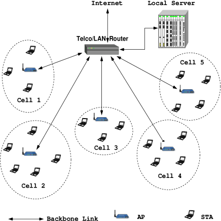
Figure 1: A multi-cell infrastructure WLAN: DCF is used only for communications within the cells. Connectivity to nodes outside the cell is provided over a separate backbone which connects the APs to the Internet through a local server and a LAN router.

To support the ever-increasing user population at high access speeds, WLANs are resorting to dense deployments of APs where, for every STA, there exists an AP close to the STA with which the STA can associate at a high Physical (PHY) rate [wanet.murty_etal08dendeAP]. However, as the density of APs increases, cell sizes become smaller and, since the number of non-overlapping channels is limited, co-channel cells become closer. Nodes in two closely located co-channel cells can suppress each other’s transmissions via carrier sensing and interfere with each other’s receptions causing packet losses. Thus, capacity might sometimes degrade with increased AP density [wanet.ergin08exptIntercellInterference], [wanet.belanger07novarumReport]. Clearly, effective planning and management are essential for achieving the benefits of dense deployments of APs. It has been demonstrated that a dense deployment of APs, along with careful channel assignment and user association control, can enhance the capacity by as much as 800% [wanet.murty_etal08dendeAP]; but the technique has been tested on a small scale. Large-scale WLANs are difficult to plan and manage since good network engineering models are lacking.

Much of the earlier work on modeling WLANs deals with single-AP networks or the so-called single cells [wanet.bianchi00performance], [wanet.cali-etal00throughput-limit], [wanet.kumar_etal07new_insights]. The existing performance analyses of multi-cell WLANs (i.e., WLANs consisting of multiple APs) are mostly based either on simulations or small-/medium-scale experiments [wanet.murty_etal08dendeAP], [wanet.ergin08exptIntercellInterference], [wanet.belanger07novarumReport]. Studying large-scale WLANs by simulations and experiments is both expensive and time-consuming. It is, therefore, important to develop an analytical understanding of such WLANs in order to derive insights into the system dynamics. The insights thus obtained can be applied: (i) to facilitate planning and management, and (ii) to develop efficient adaptive schemes for making the WLANs self-organizing and self-managing. In this paper, we first develop an analytical model for 802.11-based multi-cell WLANs and then apply our model to the task of channel assignment.

Our Contributions: We make the following contributions:

• We identify a condition, which we call the Pairwise Binary Dependence (PBD) condition, under which multi-cell WLANs can be modeled at the cell level (see A.3 in Section IV).

• We develop a scalable cell level model for multi-cell WLANs with arbitrary cell topologies (Section V).

• We extend the single cell TCP analysis of [wanet.bruno08TCPeqvSatModel] to multiple interfering cells (Section V-B).

• We demonstrate how our model could be applied in conjunction with a Learning Automata (LA) algorithm for optimal channel assignment (Section VIII).

• Based on the insights provided by our analytical model, we propose a simple decentralized algorithm which can provide fast static channel assignments (Section IX).
  

Unlike the node level models [wanet.boorstyn87multihop], [wanet.garetto_etal08starvation] or the link level models [wanet.wang-kar05multihop], [wanet.durvy08bordereffect] reported earlier in the context of multi-hop ad hoc networks, our cell level model does not require modeling the activities of every single node (resp. link). Thus, the complexity of our cell level model increases with the number of cells rather than the number of nodes (resp. links). However, our model can account for the number of nodes in each cell which may differ across the cells.

We argue that the PBD condition is likely to hold in a dense deployments of APs (see Sections III and IV-A). Hence, our cell level model can be applied to obtain a first-cut understanding of large-scale WLANs.

Our cell level model is based on the channel contention model of Boorstyn et al. [wanet.boorstyn87multihop] and the transmission attempt model of [wanet.kumar_etal07new_insights]. Thus, our approach is similar to that of [wanet.garetto_etal08starvation]. However, our model of transmission attempt process is simpler (see the discussion following Equation 2) and the closed-form expressions for collision probabilities and cell throughputs that we derive are new. We also provide new insights.

Our channel assignment algorithm provides assignments that are Nash equilibria in pure strategies for the normalized network throughput maximization objective (see Section IX). Furthermore it provides an assignment in only $M$ steps where $M$ denotes the number of available channels. In contrast to prior work, our approach to channel assignment is based on the throughput metric (see the last paragraph in Section II). Our channel assignment algorithm is motivated by our analytical model which requires the knowledge of the topology of APs. However, our channel assignment algorithm requires neither any topology information nor any message passing. To be specific, our channel assignment algorithm takes the help of the network to discover an optimal assignment (in the sense mentioned above) in a completely decentralized manner.

The remainder of this paper is organized as follows. In Section II, we discuss the related literature. In Section III, we provide the motivation for our simple cell level model. In Section IV, we provide our network model and summarize our key modeling assumptions. The analytical model is developed in Section V. In Section VI, we validate our model by comparing with ns-2 simulations. In Section VII, we apply our model to compare three different channel assignments for a 12-cell network and emphasize the impact of carrier sensing in 802.11 networks. In Section VIII, we demonstrate how our analytical model could be applied along with a Learning Automata (LA) algorithm for optimal channel assignment. We propose a simple and fast decentralized channel assignment algorithm in Section IX, and summarize the conclusions in Section LABEL:sec:conclusion. Two lengthy derivations have been deferred to the appendices at the end of the paper.

II Related Literature

Modeling of multi-hop ad hoc networks is closely related to that of multi-cell WLANs. In both cases, the hidden node and the exposed node problems [wanet.roy06PCS] are known to be the two main capacity-degrading factors. Multi-hop ad hoc networks and multi-cell WLANs are much harder to model than single cells precisely because of the presence of hidden and exposed nodes. Since the evolution of activities of each node is, in general, statistically different from that of the others’, one needs to model the system at the node level [wanet.boorstyn87multihop], [wanet.garetto_etal08starvation], or at the link level [wanet.wang-kar05multihop], [wanet.durvy08bordereffect], i.e., the activities of every single node or link and the interactions among them need to be modeled.

In the context of CSMA based multi-hop packet radio networks, Boorstyn et al. [wanet.boorstyn87multihop] proposed a Markovian model with Poisson packet arrivals and arbitrary packet length distributions. Wang and Kar [wanet.wang-kar05multihop] adopted the node level Boorstyn model to develop a link level model for 802.11 networks and studied the fairness issues. As a simplification, they assumed a fixed contention window. Garetto et al. [wanet.garetto_etal08starvation] extended the Boorstyn model to multi-hop 802.11 networks. They computed the packet loss probabilities and the throughputs per node accounting for the details of the 802.11 protocol. In particular, they incorporated the evolution of contention windows, which was missing in [wanet.wang-kar05multihop], by applying the analysis of [wanet.kumar_etal07new_insights]. However, a direct application of the Boorstyn model required two different activation rates, namely, $\lambda$ and $g$, which complicated their model (see the discussion following Equation 2). We develop a simpler model by slightly modifying the Boorstyn contention model and making it particularly suitable for 802.11 networks.

In the context of multi-cell infrastructure WLANs, Nguyen et al. [wanet.nguyen07stochGeom] proposed a model for dense 802.11 networks. To keep their interference analysis tractable, they assumed all the APs in the WLAN to be operating on the same channel. Recently, Bonald et al. [wanet.bonald08multicellprocsharing] applied the concept of “exclusion region” to model a multi-AP WLAN as a network of multi-class processor-sharing queues with state-dependent service rates. The concept of “exclusion domains” has also been applied in [wanet.durvy08bordereffect] to study the long-term fairness properties of large networks. The concept of exclusion says that, among a set of links that are in conflict, at most one can be active at any point of time. As argued in [wanet.durvy08bordereffect] and [wanet.bonald08multicellprocsharing], exclusion can be enforced in 802.11 networks by the RTS/CTS mechanism. However, suppression of interferers by RTS/CTS is not perfect because: (1) RTS frames can also collide and they must be retransmitted to enforce exclusion, (2) the overheads due to RTS/CTS that are transmitted at low rates and the capacity wastage due to RTS collisions might be significant especially when data payloads are transmitted at high rates, and most importantly, (3) RTS/CTS cannot completely eliminate hidden node collisions since nodes that cannot decode the CTS frames may collide with DATA frames that are longer than the Extended Inter Frame Space (EIFS). Thus, “exclusion” is strongly dependent on the virtual carrier sensing enforced by the RTS/CTS mechanism and is, essentially, a modeling approximation which ignores the possibility of hidden node collisions. The ineffectiveness of RTS/CTS is well known [wanet.xuGerla-etal02RTS-CTS-effectiveness] and Basic Access can outperform RTS/CTS at high data rates even when hidden nodes are present [wanet.tinnirello-etal05RTS-CTS-effectiveness].

Channel assignment in WLANs has been extensively studied (see, e.g., [wanet.leung_kim03_freq_assignment], [FAP.mishra06clientdriven], [FAP.mishra06Maxchop], [wanet.leith_clifford06CFL], [wanet.kauffmann07selfOrganization], [wanet.villegas_etal08WiComMobCom] and the references therein). Much of the existing work on channel assignment proposes to minimize the global interference power or maximize the global Signal to Noise and Interference Ratio (SINR) without taking into account the combined effect of the PHY and the MAC layers. Due to carrier sensing, nodes in 802.11 networks get opportunity to transmit for only a fraction of time, and this must be accounted for when computing the global interference power or SINR. Such an approach is found only in [wanet.leung_kim03_freq_assignment] where the authors propose to maximize a quantity called “effective channel utilization”. In reality, however, end users are more interested in the “throughputs” and, ideally, the objective should be to maximize the sum utility of throughputs. A heuristic method for computing throughputs can be found in [wanet.villegas_etal08WiComMobCom] where the authors assume long term fairness among the nodes that are mutually interfering. The heuristic adopted in [wanet.villegas_etal08WiComMobCom] says that, ignoring collisions and channel errors, a node obtains approximately $\frac{1}{n}$ of the maximum capacity where $n$ denotes the cardinality of the maximum clique to which the node belongs. In reality, the size of the maximum clique to which a node belongs can be very different from the size of the maximum clique to which one of its interfering neighbor belongs, and this leads to inconsistent predictions for node throughputs. Nevertheless, the authors in [wanet.villegas_etal08WiComMobCom] claim that, their heuristic can predict the global throughput quite well even though individual node throughputs may not be. We remark that, the multi-cell model in [wanet.bonald08multicellprocsharing] does not actually model the DCF contention and adopts a model of capacity sharing similar to the heuristic of [wanet.villegas_etal08WiComMobCom].

In summary, due to the inherent complexity of the problem, simplifying assumptions have often been made to develop tractable analytical model. The common simplification is to ignore hidden node collisions through suitable assumptions. We also ignore hidden node collisions to develop our model. However, unlike [wanet.bonald08multicellprocsharing], our model can be applied either with the Basic Access mechanism or with the RTS/CTS mechanism provided that the PBD condition holds (see A.3 in Section IV). To our knowledge, an accurate throughput based approach which accounts for PHY-MAC interactions does not exist. Thus, we first develop a simple and accurate throughput model for multi-cell WLANs and then apply our model to the task of channel assignment.

III Motivation for a Cell Level Model

In a dense deployment of APs with denser user population, it seems practically impossible to apply a node or a link level model for planning and managing the network. However, we can exploit a specific characteristics of dense deployments. Let $R$ denote the cell radius, i.e., $R$ is the maximum distance between an AP and the STAs associated to it. Let $R_{cs}$ denote the carrier sensing range, i.e., $R_{cs}$ is the distance up to which carrier sensing is effective. We observe that, ${R_{cs}>>R}$ is likely to hold in a dense deployment of APs where, for every STA, there is an AP very close to the STA. With ${R_{cs}>>R}$, the network model can be simplified in the following ways:

1. Since any transmitter ‘T’ is within a small distance $R$ from its receiver ‘R’, a node ‘H’ that is beyond a distance $R_{cs}$ from ‘T’ (i.e., a hidden node) is unlikely to interfere with ‘R’, i.e., carrier sensing would avoid much of the co-channel interference and we may ignore collisions due to hidden nodes.

2. If Node-1 in Cell-1 can sense the transmissions by Node-2 in Cell-2, then it is likely that all the nodes in Cell-1 can sense the transmissions from all the nodes in Cell-2 and vice versa, i.e., we may assume that nodes belonging to the same cell have an identical view of the rest of the network and interact with the rest of the network in an identical manner. Figure 2 summarizes this idea.

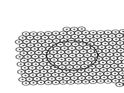
Figure 2: A dense AP network: Small circular areas represent cells with radius $R$. APs are shown as tiny circles at the centers of the cells. The big circular disk represents the area covered by the carrier sensing range $R_{cs}$ of one of the APs. Observe that, with $R_{cs}>>R$, other cells are either almost completely covered or almost not covered at all through carrier sensing. This indicates that, with $R_{cs}>>R$, nodes belonging to the same cell “perceive” identical medium activities, at least approximately.

The assumption that the AP and all its associated STAs have an identical view of the network has been applied in a dense AP setting [wanet.murty_etal08dendeAP] where the authors approximate STA statistics by statistics collected at the APs for efficiently managing their network. We adopt this idea of [wanet.murty_etal08dendeAP] to develop an analytical model. We identify the locations of the STAs with the locations of their respective APs, and treat a cell as a single entity, thus yielding a scalable cell level model. Unlike a node level model, the complexity of a cell level model increases with the number of cells rather than number of nodes. A simple cell level model is particularly suitable for the task of channel assignment since channels are assigned to cells rather than to nodes. The foregoing simplification is extremely useful at the network planning stage when the locations of the STAs are not known but the locations of the APs and the expected number of users per cell might be known. Furthermore, since much of the traffic in today’s WLANs is downlink, i.e., from the APs to the STAs, a large fraction of channel time is occupied by transmissions from the APs. It is then reasonable to develop a model based only on the topology of the APs and the expected number of users per cell assuming that the users are located close to their respective APs.

The appropriate locations for placing the APs can be decided using standard RF tools and the physical topology of the APs can be determined. Given the physical topology of the APs and a channel assignment, we can obtain the logical topology, i.e., the topology of the co-channel APs corresponding to every channel. Given a logical topology, our analytical model can predict the cell throughputs accounting for the expected number of users per cell. The cell throughputs thus obtained can provide the goodness of the assignment to a channel assignment algorithm based on which the algorithm can determine a better channel assignment. Given the logical topology with the new channel assignment, our model can provide the modified feedback and this procedure can be repeated several times to arrive at an optimal assignment. We explain this approach in Section VIII where we apply our model in conjunction with a Learning Automata (LA) based algorithm for optimal channel assignment.

IV Network Model and Assumptions

We consider scenarios with $R_{cs}>>R$. Based on our earlier discussion, we assume that simultaneous transmissions by nodes that are farther than $R_{cs}$ from each other results in successful receptions at their respective receivers. We also assume that simultaneous transmissions by nodes that are within $R_{cs}$ always lead to packet losses at their respective receivers, i.e., we ignore the possibility of packet capture. For simplicity, we assume symmetry among the nodes and of the propagation environment. In particular, this means that (i) nodes use identical protocol parameters (e.g., contention windows, retry limit etc.), and (ii) if Node-1 can sense Node-2, then Node-2 can also sense Node-1.

We say that two nodes are dependent if they are within $R_{cs}$; otherwise, the two nodes are said to be independent. Two cells are said to be independent if every node in a cell is independent w.r.t. every node in the other cell; otherwise, the two cells are said to be dependent. Two dependent cells are said to be completely dependent if every node in a cell is dependent w.r.t. every node in the other cell. In this broad setting, our key assumptions are the following:

1. Only non-overlapping channels are used.

2. Associations of STAs with APs are static. This implies that the number of STAs in a cell is fixed.

3. Pairwise Binary Dependence (PBD): Any pair of cells is either independent or completely dependent.

4. The STAs are so close to their respective APs that packet losses due to channel errors are negligible.

5. The EIFS deferral has been disabled in the sense that medium access always starts after a Distributed Inter-Frame Space (DIFS) deferral.

IV-A Discussion of the PBD Condition and Assumption A.5

The PBD condition is crucial to the analytical model being developed in this paper. It includes the possibility that two given co-channel cells can be independent, i.e., two co-channel cells can be so far apart that activities in one cell do not affect the activities in the other cell. However, if two cells are dependent, the PBD condition rules out the possibility that only a subset of nodes in one cell can sense a subset of nodes in the other cell. We note that, in a dense deployment of APs, due to small cell radius $R$ and $R_{cs}>>R$, complete dependence would hold up to $R_{cs}$ and independence would hold beyond $R_{cs}$, i.e., the PBD condition would hold, at least approximately. The PBD condition is a geometric property that enables modeling at the cell level since, if the PBD condition holds, the relative locations of the nodes within a cell do not matter. Also, any interferer ‘I’, which must be within $R_{cs}$ of a receiver ‘R’, will also be within $R_{cs}$ of the transmitter ‘T’ if the PBD condition holds. Hence, either (i) ‘I’ can start transmitting at the same time as ‘T’ causing synchronous collisions at ‘R’, or (ii) ‘I’ gets suppressed by T’s RTS (or DATA) transmission followed by R’s CTS (or ACK) transmission since CTS and ACK frames are given higher priority through SIFS ($<$ DIFS $<$ EIFS). Thus, if the PBD condition holds, nodes do not require deferral by EIFS; deferral by DIFS would suffice. Thus, we assume that contention for medium access always begins after deferral by DIFS and we do not model the impact of EIFS. We remark that certain commercial products, e.g., Atheros cards, have user-configurable EIFS and EIFS can be easily disabled in such devices.

V Analysis of Multi-Cell WLANs with Arbitrary Cell Topology

In this section, we develop a cell level model for WLANs that satisfy the PBD condition. We provide a generic model and demonstrate the accuracy of our model by comparing with simulations of specific cell topologies pertaining to: (i) networks with linear or hexagonal layout of cells (see Figures 3-3), and (ii) networks with arbitrary layout of cells (see Figure 3). We index the cells by positive integers $1,2,\ldots,N$, in some arbitrary fashion where $N$ denotes the number of cells. Two completely dependent co-channel cells are said to be neighbours. Note that, two completely dependent cells operating on different non-overlapping channels are not neighbors. Let $\mathcal{N}=\{1,2,\ldots,N\}$ denote the set of cells and $\mathcal{N}_{i}\;(\subset\mathcal{N})$ denote the set of neighboring cells of Cell-$i$ $(i\in\mathcal{N})$. Note that $i\notin\mathcal{N}_{i}$. Given the location of the APs and a channel assignment, we can obtain the set of neighboring cells for each cell. The key to modeling the cell level contention is the cell level contention graph $\mathcal{G}$ which is obtained by representing every cell by a vertex and joining every pair of neighbors by an edge. Figures 3-3 also depict the contention graphs corresponding to each cell topology.

In Section V-A, we model the case where nodes are infinitely backlogged and are transferring packets to one or more nodes in the same cell using UDP connection(s). Notice that single-hop direct communications among the STAs in the same cell without involving the AP are also allowed. In Section V-B, we extend to the case when STAs download long files through their respective APs using persistent TCP connections.

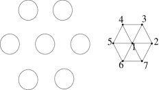
Figure 3: Examples of multi-cell systems: (a) four linearly placed co-channel cells, (b) five linearly placed co-channel cells, (c) seven hexagonally placed co-channel cells, and (d) seven co-channel cells with an arbitrary cell topology. The cell level contention graphs have also been shown where the dots represent the cells. Neighbors have been joined by edges. For example (a), the pairs $\{1,2\}$, $\{2,3\}$ and $\{3,4\}$ are dependent and the pairs $\{1,3\}$, $\{1,4\}$ and $\{2,4\}$ are independent.

V-A Modeling with Saturated MAC Queues

Due to the PBD condition, nodes belonging to the same cell have an identical view of the rest of the network. When one node senses the medium idle (resp. busy) so do the other nodes in the same cell and we say that a cell is sensing the medium idle (resp. busy). Since the nodes are saturated, whenever a cell senses the medium idle, all the nodes in the cell decrement their back-off counters per idle back-off slot that elapses in their local medium and we say that the cell is in back-off. If the nodes were not saturated, a node with an empty MAC queue would not count down during the “medium idle” periods and the number of contending nodes would be time-varying. With saturated AP and STA queues, the number of contending nodes in each cell remains constant.

We say that a cell transmits when one or more nodes in the cell transmit(s). When two or more nodes in the same cell transmit, an intra-cell collision occurs. Consider Figure 3. There are periods during which all the four cells are in back-off. We model these periods, when none of the cells is transmitting, by the state $\Phi$ where $\Phi$ denotes the empty set. The system remains in State $\Phi$ until one or more cell(s) transmit(s). When a cell transmits, its neighbors sense the transmission after a propagation delay and they defer medium access. We then say that the neighbors are blocked due to carrier sensing. However, two neighboring cells can start transmitting together before they could sense each other’s transmissions resulting in synchronous inter-cell collisions.

We observe that a cell can be in one of the three states: (i) transmitting, (ii) blocked, or (iii) in back-off. Modeling the synchronous inter-cell collisions requires a discrete time slotted model. However, this would require a large state space since the cells change their states in an asynchronous manner. For example, consider Figure 3 and suppose that Cell-1 starts transmitting and blocks Cell-2 after a propagation delay. However, Cell-3 is independent of Cell-1 and can start transmitting at any instant during Cell-1’s transmission. Thus, the evolution of the system is partly asynchronous and partly synchronous. To capture both, we follow a two-stage approach along the lines of [wanet.garetto_etal08starvation]. In the first stage, we ignore inter-cell collisions and assume that blocking due to carrier sensing is immediate. We develop a continuous time model as in [wanet.boorstyn87multihop] to obtain the fraction of time each cell is transmitting/blocked/in back-off. In the second stage, we obtain the fraction of slots in which various subsets of neighboring cells can start transmitting together. This would allow us to compute the collision probabilities accounting for synchronous inter-cell collisions. We combine the above through a fixed-point equation and compute the throughputs using the solution of the fixed-point equation. We define the following [wanet.kumar_etal07new_insights]:

$n_{i}:=$ number of nodes in Cell-$i$

$\beta_{i}:=$ (transmission) attempt probability (over the back-off slots) of the nodes in Cell-$i$

$\gamma_{i}:=$ collision probability as seen by the nodes in Cell-$i$ (conditioned on an attempt being made)

Let $A_{i}(T)$ denote the cumulative number of attempts made by a tagged node (any node due to symmetry) in Cell-$i$ up to time $T$. Let $C_{i}(T)$ denote the cumulative number of collisions as seen by the tagged node up to time $T$. Let $B_{i}(T)$ denote the cumulative number of back-off slots elapsed in Cell-$i$ up to time $T$. Then, the attempt probability $\beta_{i}$ and the (conditional) collision probability $\gamma_{i}$ of the tagged node are more precisely defined by

$$\beta_{i}:=\lim_{T\rightarrow\infty}\frac{A_{i}(T)}{B_{i}(T)}\;;\;\gamma_{i}:=\lim_{T\rightarrow\infty}\frac{C_{i}(T)}{A_{i}(T)}\;.$$

Note that $\beta_{i}$ is the attempt probability of the nodes in Cell-$i$, irrespective of whether the nodes in the other cells can also attempt. This is a simplification and can be viewed as an extension to the decoupling approximation introduced in [wanet.bianchi00performance]. Using the decoupling approximation and the analysis in [wanet.kumar_etal07new_insights], the attempt probability $\beta_{i}$ of the nodes in Cell-$i$, $\forall i\in\mathcal{N}$, can be related to $\gamma_{i}$ as

$$\beta_{i}=G(\gamma_{i}):=\frac{1+\gamma_{i}\ldots+\gamma_{i}^{K}}{b_{0}+\gamma_{i}b_{1}\ldots+\gamma_{i}^{k}b_{k}+\ldots+\gamma_{i}^{K}b_{K}}$$ (1)

where $K$ denotes the retry limit and $b_{k}$, $0\leq k\leq K$, denotes the mean back-off sampled after $k$ collisions.

The First Stage: When Cell-$i$ and some (or all) of its neighboring cells are in back-off their (cell level) attempt processes compete until one of the cells, say, Cell-$j$, ${j\in\mathcal{N}_{i}\cup\{i\}}$, transmits. Since, we ignore inter-cell collisions in the first stage, the possibility of two or more neighboring cells attempting together is ruled out. When Cell-$i$ wins the contention, we say that it has become active. When Cell-$i$ becomes active, it gains the control over its local medium by immediately blocking its neighboring cells that are not yet blocked. We assume that the time until Cell-$i$ goes from the back-off state to the active state is exponentially distributed with mean $\frac{1}{\lambda_{i}}$. The activation rate $\lambda_{i}$ is given by

$$\lambda_{i}=\frac{1-(1-\beta_{i})^{n_{i}}}{\sigma}$$ (2)

where $\sigma$ denotes the duration of a back-off slot (in seconds) and $1-(1-\beta_{i})^{n_{i}}$ is the probability that there is an attempt in Cell-$i$ per back-off slot. Notice that we have converted the aggregate attempt probability in a cell per back-off slot to an attempt rate over back-off time. Also notice that, our assumption of exponential “time until transition from the back-off state to the active state” is the continuous time analogue of the assumption of geometric “number of slots until attempt” in the discrete time models of [wanet.cali-etal00throughput-limit] and [wanet.kumar_etal07new_insights].

Discussion V.1

In [wanet.garetto_etal08starvation], the authors use an unconditional activation rate $\lambda$ over all times as well as a conditional activation rate $g$ over the back-off times and relate the two rates through a throughput equation which makes their model unnecessarily complicated. The activation rate $\lambda$ in our model is conditional on being in the back-off state. Thus, we use a single activation rate and our model is much simpler than that of [wanet.garetto_etal08starvation]. Our modified approach can also be applied to simplify the node level model of [wanet.garetto_etal08starvation]. ∎

When Cell-$i$ becomes active, it remains active and its neighbors remain blocked due to Cell-$i$ until Cell-$i$’s transmission finishes and an idle DIFS period elapses. The active periods of Cell-$i$ are of mean duration $\frac{1}{\mu_{i}}$. When Cell-$i$ becomes active through a successful transmission (resp. an intra-cell collision) its neighbors remain blocked due to Cell-$i$ for a success time $T_{s}$ (resp. a collision time $T_{c}$). Hence, $\frac{1}{\mu_{i}}$ is given by

$$\frac{1}{\mu_{i}} = \left(\frac{n_{i}\beta_{i}(1-\beta_{i})^{n_{i}-1}}{1-(1-\beta_{i})^{n_{i}}}\right)\cdot(T_{s})$$ (3)

$$+\;\left(1-\frac{n_{i}\beta_{i}(1-\beta_{i})^{n_{i}-1}}{1-(1-\beta_{i})^{n_{i}}}\right)\cdot(T_{c})$$

where $\displaystyle\frac{n_{i}\beta_{i}(1-\beta_{i})^{n_{i}-1}}{1-(1-\beta_{i})^{n_{i}}}$ is the probability that Cell-$i$ becomes active through a success given that it becomes active.

Due to carrier sensing, at any point of time, only a set ${\mathcal{A}\;(\subset\mathcal{N})}$ of mutually independent cells can be active together, i.e., $\mathcal{A}$ must be an independent set (of vertices) of the contention graph $\mathcal{G}$. From the contention graph $\mathcal{G}$, we can determine the set of cells $\mathcal{B}_{\mathcal{A}}$ that get blocked due to $\mathcal{A}$, and the set of cells $\mathcal{U}_{\mathcal{A}}$ that remain in back-off, i.e., the set of cells in which nodes can continue to decrement their back-off counters. Note that $\mathcal{A}$, $\mathcal{B}_{\mathcal{A}}$ and $\mathcal{U}_{\mathcal{A}}$ form a partition of $\mathcal{N}$, i.e., $\mathcal{A}$, $\mathcal{B}_{\mathcal{A}}$ and $\mathcal{U}_{\mathcal{A}}$ are pairwise disjoint and $\mathcal{N}=\mathcal{A}\cup\mathcal{B}_{\mathcal{A}}\cup\mathcal{U}_{\mathcal{A}}$.

Figure 4: The CTMC describing the cell level contention for the four linearly placed cells given in Figure 3.

We take $\mathcal{A}(t)$, i.e., the set $\mathcal{A}$ of active cells at time $t$, as the state of the multi-cell system at time $t$. It is worthwhile now to mention the insensitivity result of Boorstyn et al. [wanet.boorstyn87multihop] which says that the product-form solution provided by their model is insensitive to the packet length distribution and depends only on the mean packet lengths. Applying their insensitivity argument, we take the active periods of Cell-$i$ to be i.i.d. exponential random variables with mean $\frac{1}{\mu_{i}}$. Due to exponential activation rates and active periods, at any time $t$, the rate of transition to the next state is completely determined by the current state $\mathcal{A}(t)$. For example, Cell-$j$, $j\in\mathcal{U}_{\mathcal{A}}$, joins the set $\mathcal{A}$ (and its neighboring cells that are also in $\mathcal{U}_{\mathcal{A}}$ join the set $\mathcal{B}_{\mathcal{A}}$) at a rate $\lambda_{j}$. Similarly, Cell-$i$, $i\in\mathcal{A}$, leaves the set $\mathcal{A}$ (and its neighboring cells that are blocked only due to Cell-$i$ leave the set $\mathcal{B}_{\mathcal{A}}$) to join the set $\mathcal{U}_{\mathcal{A}}$ at a rate $\mu_{i}$. In summary, the process $\{\mathcal{A}(t),t\geq 0\}$ has the structure of a Continuous Time Markov Chain (CTMC). This CTMC contains a finite number of states and is irreducible. Hence, it is stationary and ergodic. The set of all possible independent sets which constitutes the state space of the CTMC $\{\mathcal{A}(t),t\geq 0\}$ is denoted by $\mathcal{A}$. For a given contention graph, $\mathcal{A}$ can be determined. For the topology given in Figure 3, we have $\mathcal{N}=\{1,2,3,4\}$ and $\mbox{\boldmath$\mathcal{A}$}=\{\Phi,\{1\},\{2\},\{3\},\{4\},\{1,3\},\{1,4\},\{2,4\}\}$ where we recall that $\Phi$ denotes the empty set. The CTMC $\{\mathcal{A}(t),t\geq 0\}$ corresponding to this example is given in Figure 4.

It can be checked that the transition structure of the CTMC $\{\mathcal{A}(t),t\geq 0\}$ satisfies the Kolmogorov Criterion for reversibility (see [theory.kelly79reversibility]). Hence, the stationary probability distribution $\pi(\mathcal{A}),\mathcal{A}\in\mbox{\boldmath$\mathcal{A}$}$, satisfies the detailed balance equations,

$$\pi(\mathcal{A})\lambda_{i}=\pi(\mathcal{A}\cup\{i\})\mu_{i}\;,\;(\forall i\in\mathcal{U}_{\mathcal{A}})$$

and the stationary probability distribution has the form

$$\pi(\mathcal{A})=\left(\prod_{i\in\mathcal{A}}\rho_{i}\right)\pi(\Phi),\;\;\;(\forall\mathcal{A}\in\mbox{\boldmath$\mathcal{A}$})$$ (4)

where $\rho_{i}:=\frac{\lambda_{i}}{\mu_{i}}$ and $\pi(\Phi)$ (which denotes the stationary probability that none of the cells is active) is determined from the normalization equation

$$\sum_{\mathcal{A}\in\mbox{\boldmath$\mathcal{A}$}}\pi(\mathcal{A})=1.$$ (5)

Combining Equations 4 and 5, we obtain

$$\pi(\mathcal{A})=\displaystyle\frac{\left(\displaystyle\prod_{i\in\mathcal{A}}\rho_{i}\right)}{\displaystyle\sum_{\mathcal{A}\in\mbox{\boldmath$\mathcal{A}$}}\left(\displaystyle\prod_{j\in\mathcal{A}}\rho_{j}\right)},\;\;\;(\forall\mathcal{A}\in\mbox{\boldmath$\mathcal{A}$})$$ (6)

Convention: A product $\prod$ over an empty index set is taken to be equal to 1. Notice that, with this convention, Equation 6 holds for $\pi(\Phi)$ as well.

$$\gamma_{i}=\frac{\sum_{\mathcal{A}\in\mbox{\boldmath$\mathcal{A}$}\;:\;i\in\mathcal{U}_{\mathcal{A}}}\pi(\mathcal{A})\left[1-(1-\beta_{i})^{n_{i}-1}\prod_{j\in\mathcal{N}_{i}\;:\;j\in\mathcal{U}_{\mathcal{A}}}(1-\beta_{j})^{n_{j}}\right]}{\sum_{\mathcal{A}\in\mbox{\boldmath$\mathcal{A}$}\;:\;i\in\mathcal{U}_{\mathcal{A}}}\pi(\mathcal{A})}\;\;\;\;\;\;\;\;\;\;\;\;(\forall i\in\mathcal{N})$$ (7)

 

The Second Stage: We now compute the collision probabilities $\gamma_{i}$’s accounting for inter-cell collisions. Note that $\gamma_{i}$ is conditional on an attempt being made by a node in Cell-$i$. Hence, to compute $\gamma_{i}$, we focus only on those states in which Cell-$i$ can attempt. Clearly, Cell-$i$ can attempt in State-$\mathcal{A}$ iff it is in back-off in State-$\mathcal{A}$, i.e., iff $i\in\mathcal{U}_{\mathcal{A}}$. In all such states a node in Cell-$i$ can incur intra-cell collisions due the other nodes in Cell-$i$. Furthermore, some (or all) of Cell-$i$’s neighbors might also be in back-off in State-$\mathcal{A}$. If a neighboring cell, say, Cell-$j$, $j\in\mathcal{N}_{i}$, is also in back-off in State-$\mathcal{A}$, i.e., if $j\in\mathcal{U}_{\mathcal{A}}$, then a node in Cell-$i$ can incur inter-cell collisions due to the nodes in Cell-$j$. The collision probability $\gamma_{i}$ is then given by Equation 7 (appears at the top of the next page). A formal derivation of Equation 7 is provided in Appendix LABEL:app:derivation-eqn-gamma_i.

Fixed Point Formulation: Equations 2, 3, 6, 7 and $\rho_{i}:=\frac{\lambda_{i}}{\mu_{i}}$ can express the $\gamma_{i}$’s as functions of only the $\beta_{i}$’s. Together with Equation 1, they yield an $N$-dimensional fixed point equation where we recall that $N$ is the total number of cells. The $N$-dimensional fixed point equation can be numerically solved to obtain the collision probabilities $\gamma_{i}$’s, the attempt probabilities $\beta_{i}$’s and the stationary probabilities $\pi(\mathcal{A})$’s. In all of the cases that we have considered, the fixed point iterations were observed to converge to the same solutions irrespective of starting points. However, we have not yet been able to analytically prove the uniqueness of solutions.

Calculating the Throughputs: The stationary probabilities of the CTMC $\{\mathcal{A}(t),t\geq 0\}$ can provide the fraction of time $x_{i}$ for which Cell-$i$ is unblocked. A cell is said to be unblocked when it belongs to either $\mathcal{A}$ or $\mathcal{U}_{\mathcal{A}}$. Thus, $\forall i\in\mathcal{N}$,

$$x_{i}=\sum_{\mathcal{A}\in\mbox{\boldmath$\mathcal{A}$}\;:\;i\in\mathcal{A}\cup\mathcal{U}_{\mathcal{A}}}\pi(\mathcal{A}).$$ (8)

Definition V.1

Let $\mathcal{G}_{i}$, $i\in\mathcal{N}$, denote the subgraph obtained by removing Cell-$i$ and its neighboring cells in $\mathcal{N}_{i}$ from the contention graph $\mathcal{G}$. For a given contention graph $\mathcal{G}$, let $\Delta$ be defined as follows:

$$\Delta:=\sum_{\mathcal{A}\in\mbox{\boldmath$\mathcal{A}$}}\left(\prod_{j\in\mathcal{A}}\rho_{j}\right)$$ (9)

Let $\Delta_{i}$ denote the $\Delta$ corresponding to the subgraph $\mathcal{G}_{i}$. ∎

An important observation which facilitates the computation of the $x_{i}$’s is given by the following theorem.

Theorem V.1

The fraction of time $x_{i}$ for which Cell-$i$ is unblocked is given by

$$x_{i}=\frac{(1+\rho_{i})\Delta_{i}}{\Delta},\;\;\;\;\;\forall i\in\mathcal{N}.$$ (10)

Proof:

See Appendix LABEL:app:derivation-theorem-xi. ∎

Let $\Theta_{i}$ denote the aggregate throughput of Cell-$i$ in a given multi-cell network and let $\Theta_{n_{i},singlecell}$ denote the aggregate throughput of Cell-$i$ if it was an isolated cell containing $n_{i}$ nodes. Both $\Theta_{i}$ and $\Theta_{n_{i},singlecell}$ are in packets/sec. We approximate $\Theta_{i}$ by

$$\Theta_{i} = x_{i}\cdot\Theta_{n_{i},singlecell}$$ (11)

$$= \frac{(1+\rho_{i})\Delta_{i}}{\Delta}\cdot\Theta_{n_{i},singlecell},$$

and $\Theta_{i}$ divided by $n_{i}$ gives the per node throughput $\theta_{i}$ in Cell-$i$, i.e., $\theta_{i}=\frac{\Theta_{i}}{n_{i}}$ (packets/sec).

Discussion V.2

Equation 11 is justified as follows. If Cell-$i$ is indeed independent of every other cell in the network, it is never blocked and does not incur inter-cell collisions. Then, we have $x_{i}=1$ and $\Theta_{i}=\Theta_{n_{i},singlecell}$. However, in general, Cell-$i$ gets blocked due to its neighbors for a fraction of time $1-x_{i}$ and remains unblocked for a fraction of time $x_{i}$. If we ignore the time wasted in inter-cell collisions, the times during which Cell-$i$ is unblocked would consist only of the back-off slots and the activities of Cell-$i$ by itself. Thus, we approximate the aggregate throughput of Cell-$i$, over the times during which it is unblocked, by $\Theta_{n_{i},singlecell}$ and $\Theta_{n_{i},singlecell}$ multiplied with $x_{i}$ gives the aggregate throughput $\Theta_{i}$ of Cell-$i$ in the multi-cell network. ∎

Clearly, Equation 11 is an approximation since the time wasted in inter-cell collisions have been ignored. However, we prefer to keep the approximation because: (1) it is quite accurate when compared with the simulations (see Section VI), and (2) it can be efficiently computed since $\Theta_{n_{i},singlecell}$ follows from a single cell analysis and the $\Delta$ as well as the $\Delta_{i}$’s can be computed using efficient algorithms [wanet.kershenbaum-etal87complex].

Complexity of the Model: In general, obtaining the state space $\mathcal{A}$ by searching for all possible independent sets $\mathcal{A}$ could be computationally expensive and the complexity grows exponentially with the number of vertices in the contention graph [wanet.kershenbaum-etal87complex]. For realistic topologies, where connectivity in the contention graph is related to distance in the physical network, efficient computation of $\mathcal{A}$ is possible up to several hundred vertices in the contention graph [wanet.kershenbaum-etal87complex]. Thus, a cell level model is extremely helpful in analyzing large-scale WLANs with hundreds of cells since, unlike a node level model, each vertex in the contention graph now represents a cell.

Large $\rho$ Regime: Let $\eta$ (resp. $\eta_{i}$) denote the number of Maximum Independent Sets (MISs) of $\mathcal{G}$ (resp. $\mathcal{G}_{i}$) (see Definition V.1). Notice that, $\eta_{i}$ is also equal to the number of MISs of $\mathcal{G}$ to which Cell-$i$ belongs. From Equation 6 it is easy to see that, as $\rho_{i}\rightarrow\infty$, $\forall i\in\mathcal{N}$, we have,

$$\pi(\mathcal{A})\rightarrow\left\{\begin{array}[]{ll}\displaystyle\frac{1}{\eta}&\mbox{if $\mathcal{A}$ is an MIS,}\\ 0&\mbox{otherwise}.\end{array}\right.$$

Also, from Equations 8, 9 and 10, we observe that, as ${\rho_{i}\rightarrow\infty}$, $\forall i\in\mathcal{N}$, we have,

$$x_{i}\rightarrow\displaystyle\frac{\eta_{i}}{\eta}\;,$$

where we recall that $x_{i}$ is the fraction of time for which Cell-$i$ is unblocked. The quantity

$$x_{i}=\displaystyle\frac{\Theta_{i}}{\Theta_{n_{i},singlecell}}$$

can be interpreted as the throughput of Cell-$i$, normalized with respect to Cell-$i$’s single cell throughput. We define the normalized network throughput $\bar{\Theta}$ by

$$\bar{\Theta}:=\sum_{i=1}^{N}x_{i}.$$ (12)

Clearly, as $\rho_{i}\rightarrow\infty$, $\forall i\in\mathcal{N}$, the cells that belong to every MIS of the contention graph obtain normalized throughput 1 and the cells that do not belong to any MIS obtain normalized throughput 0. Similar observations have also been made in [wanet.wang-kar05multihop]. We further observe that, as $\rho_{i}\rightarrow\infty$ for all $i\in\mathcal{N}$, only an MIS of cells can be active at any point of time. Since an MIS is always active, as $\rho_{i}\rightarrow\infty$, $\forall i\in\mathcal{N}$, we have,

$$\bar{\Theta}\rightarrow\alpha(\mathcal{G})\;,$$

where $\alpha(\mathcal{G})$ denotes the cardinality of an MIS of $\mathcal{G}$ and is also called the independence number of $\mathcal{G}$. Notice that $\alpha(\mathcal{G})$ is a measure of spatial reuse in the network.

V-B Extension to TCP Traffic

We now extend the analysis of Section V-A to the more realistic case when users access a local proxy server via persistent TCP connections. Our extension to TCP-controlled long file downloads is based on the single cell TCP-WLAN interaction model of [wanet.bruno08TCPeqvSatModel]. The model proposed in [wanet.bruno08TCPeqvSatModel] has been shown to be quite accurate when: (1) the local proxy server is connected with the AP by a relatively fast wired LAN such that the AP in the WLAN is the bottleneck, (2) every STA has a single persistent TCP connection, (3) there are no packet losses due to buffer overflow, (4) the TCP timeouts are set large enough to avoid timeout expirations due to Round Trip Time (RTT) fluctuations, and (5) the delayed ACK mechanism is disabled. We keep the above assumptions in this paper.

In [wanet.bruno08TCPeqvSatModel], the authors propose to model a single cell having an AP and an arbitrary number of STAs with long-lived TCP connections by an “equivalent saturated network” which consists of a saturated AP and a single saturated STA. “This equivalent saturated model greatly simplifies the modeling problem since the TCP flow control mechanisms are now implicitly hidden and the total throughput can be computed using the saturation analysis [wanet.bruno08TCPeqvSatModel].” Using the equivalent saturated model of [wanet.bruno08TCPeqvSatModel], the analysis of Section V-A can be applied to TCP-controlled long file downloads, taking $n_{i}=2,\forall i\in\mathcal{N}$. We explain the intuition behind this straightforward extension in the following.

The equivalent saturated model of [wanet.bruno08TCPeqvSatModel] is quite accurate in the single cell scenario because of the following reasons. For TCP-controlled long file transfers in WLANs, the AP has to serve $n\geq 1$ STA(s) by sending TCP DATA (resp. TCP ACK) packets to $n_{d}$ downloading (resp. $n_{u}$ uploading) STAs ($n_{l}+n_{u}=n$). However, since DCF is packet fair, the AP does not get any prioritized access to the medium. Hence, in steady state, the AP’s MAC queue never becomes empty, i.e., the AP is saturated. Furthermore, since it is assumed that there are no buffer losses and no TCP timeouts, initially, the TCP windows keep growing and, in steady state (i) the TCP windows stay at their maximum, say, $W_{max}$, for every connection, and (ii) the sum of the number of packets in the AP and in the STAs is equal to $nW_{max}$. Most of these packets reside in the AP queue due to the DCF contention mentioned above and only a few STA queues remain non-empty at any point of time. It turns out that, the mean number of STAs with non-empty MAC queues $\approx$ 1.5 for sufficiently large $n$ [wanet.bruno08TCPeqvSatModel] ($n\geq 5$ suffices). Thus, the $n$ STAs can be approximated by a single saturated STA and the equivalent saturated model can still predict the throughputs quite accurately. In fact, the equivalent saturated model can also accurately predict the collision probability of the AP which is indeed saturated.

Our extension to multiple cells is based on our key observations that,

1. As in single cells, the AP continues to be saturated in multi-cell scenarios as well.

2. The number of non-empty STAs changes only at the end of successful transmissions [wanet.harsha07WiNet]; when the AP (resp. a STA) succeeds, this number increases (resp. decreases) by one.

3. Whenever a cell is blocked, its activities are frozen, and hence, the number of non-empty STAs cannot change during the blocked periods. Thus, we can strip off the blocked periods and put the unblocked periods together over which time the cell would behave like a single cell.

Applying the third observation above, the TCP download throughput of a cell, say, Cell-$i$, in the multi-cell scenario can be obtained by multiplying the single cell TCP download throughput of Cell-$i$ with the fraction of time $x_{i}$ for which Cell-$i$ is unblocked. Clearly, due to blocking, the likelihood of TCP timeouts increases. However, in our simulations, we have observed that, if the minimum value of Retransmission TimeOut (RTO) is set to 200ms (which is the default value in ns-2.31), the analytical model is capable of predicting AP statistics quite well both in the single cell and the multi-cell scenarios. In fact, cells switch between the blocked and the unblocked states at a fast time scale of few packet transmission times which takes only a few milliseconds. Hence, timeout expirations are rare given that there are no buffer losses.

VI Results and Discussion

We carried out simulations using ns-2.31 [wanet.ns2]. We created the example topologies given in Figure 3-3. We chose the cell radii and the distances among the cells such that the PBD condition holds. Nodes were randomly placed within the cells. The saturated case was simulated with high rate CBR over UDP connections. For the TCP case, we created one TCP download connection per STA. Each TCP connection was fed by an FTP source with the TCP source agent attached directly to the AP to emulate a local proxy server. The AP buffer was set large enough to avoid buffer losses. The EIFS deferral and the delayed ACK mechanism were disabled. Each case was simulated 20 times, each run for 200 sec of “simulated time”. We report the results for “Basic Access”. Similar results were obtained with “RTS/CTS”. We took 11 Mbps data rate and packet payloads of 1000 bytes. The function “fsolve()” of MATLAB was used for solving the $N$-dimensional fixed point equation.

TABLE I: Single Cell Results: Columns 2-3 Correspond to $n$ Saturated Nodes. Columns 4-7 Correspond to TCP Downloads with $n$ STAs

$n$	$\gamma_{ana}^{sat}$	$\theta_{ana}^{sat}$	$\gamma_{sim}^{AP}$	$\gamma_{ana}^{AP}$	$\theta_{sim}^{AP}$	$\theta_{ana}^{AP}$
		(pkts/sec)			(pkts/sec)	(pkts/sec)
1	0	801.78	0.0578	0.0586	454.01	456.53
2	0.0586	349.94	0.0538	0.0586	456.06	456.53
3	0.1077	236.09	0.0533	0.0586	456.09	456.53
4	0.1473	176.63	0.0528	0.0586	456.17	456.53
5	0.1812	140.29	0.0531	0.0586	456.05	456.53
6	0.2100	115.89	0.0530	0.0586	456.10	456.53
7	0.2348	98.43	0.0536	0.0586	456.88	456.53
8	0.2565	85.35	0.0531	0.0586	456.97	456.53
10	0.2927	67.11	0.0531	0.0586	456.02	456.53

Table I summarizes the results for a single cell. Columns 2-3 (resp. 4-7) correspond to the saturated case (resp. TCP download case) with $n$ saturated nodes (resp. 1 AP and $n$ STAs). The analytical results for the saturated case were obtained using [wanet.kumar_etal07new_insights] and that for the TCP case were obtained using [wanet.bruno08TCPeqvSatModel]. These single cell results obtained from known analytical models serve as the basis of our multi-cell results. The analytical throughputs per-node (resp. of AP) in Column 3 (resp. Column 7) multiplied with the $x_{i}$’s obtained from our multi-cell analysis provide the analytical throughputs per-node (resp. of AP) in the multi-cell cases (see Equation 11).

VI-A Results for the Saturated Case

TABLE II: Results for the Four Linearly Placed Cells Given in Figure 3 when Each Cell Contains $n=5$ Nodes

Cell	$\gamma_{sim}$	$\gamma_{ana}$	$\theta_{sim}$	$\theta_{ana}$	$\theta_{\infty}$
index			(pkts/sec)	(pkts/sec)	(pkts/sec)
1	0.2351	0.2399	94.48	97.41	93.53
2	0.3005	0.3146	41.21	46.66	46.76
3	0.2999	0.3146	41.66	46.66	46.76
4	0.2359	0.2399	93.99	97.41	93.53

TABLE III: Results for the Five Linearly Placed Cells Given in Figure 3 when Each Cell Contains $n=5$ Nodes

Cell	$\gamma_{sim}$	$\gamma_{ana}$	$\theta_{sim}$	$\theta_{ana}$	$\theta_{\infty}$
index			(pkts/sec)	(pkts/sec)	(pkts/sec)
1	0.1882	0.1897	129.35	131.35	140.29
2	0.3321	0.3975	8.69	8.64	0
3	0.1892	0.1925	123.35	126.41	140.29
4	0.3321	0.3975	8.72	8.64	0
5	0.1884	0.1897	129.31	131.35	140.29

TABLE IV: Results for the Seven Hexagonally Placed Cells Given in Figure 3 when Each Cell Contains $n=10$ Nodes

Cell	$\gamma_{sim}$	$\gamma_{ana}$	$\theta_{sim}$	$\theta_{ana}$	$\theta_{\infty}$
index			(pkts/sec)	(pkts/sec)	(pkts/sec)
1	0.2335	0.8896	0.003	0.02	0
2	0.3045	0.3158	31.97	32.35	33.56
3	0.3061	0.3158	31.93	32.35	33.56
4	0.3055	0.3158	32.05	32.35	33.56
5	0.3054	0.3158	31.86	32.35	33.56
6	0.3070	0.3158	32.00	32.35	33.56
7	0.3058	0.3158	31.95	32.35	33.56

TABLE V: Results for the Seven Arbitrarily Placed Cells Given in Figure 3 when Cell-$i$, $1\leq i\leq 7$ Contains $n_{i}=i+1$ Nodes

Cell	$n_{i}$	$\gamma_{sim}$	$\gamma_{ana}$	$\theta_{sim}$	$\theta_{ana}$	$\theta_{\infty}$
index $i$				(pkts/sec)	(pkts/sec)	(pkts/sec)
1	2	0.0669	0.0666	320.66	325.26	349.94
2	3	0.1163	0.1163	216.19	219.65	236.09
3	4	0.2764	0.3280	12.48	12.97	0
4	5	0.3105	0.3318	34.29	40.20	46.76
5	6	0.2505	0.2585	83.77	84.92	77.26
6	7	0.3574	0.3787	28.67	32.40	32.81
7	8	0.3062	0.3139	56.87	59.21	56.90

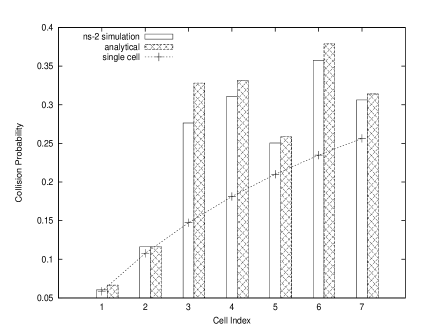
Figure 5: Comparing collision probability $\gamma$ for the example scenario in Figure 3 when Cell-$i$, $1\leq i\leq 7$, contains $n_{i}=i+1$ saturated nodes.

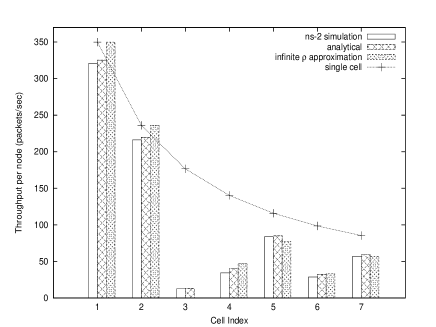
Figure 6: Comparing throughput per node $\theta$ for the example scenario in Figure 3 when Cell-$i$, $1\leq i\leq 7$, contains $n_{i}=i+1$ saturated nodes.

Tables V-V summarize the results for the example multi-cell cases depicted in Figures 3-3, respectively, when each cell contains $n$ saturated nodes. Table V summarizes the results for the example case given in Figure 3 when Cell-$i$, $1\leq i\leq 7$, contains $n_{i}=i+1$ saturated nodes. Quantities denoted with a subscript “sim” (resp. “ana”) correspond to results obtained from ns-2 simulations (resp. fixed point analysis). In each case, $\theta_{\infty}$ represents the throughput per-node obtained by taking $\rho_{i}\rightarrow\infty,\forall i\in\mathcal{N}$. We report only the mean values for our simulation results. The 99% confidence intervals were observed to be within 5% of the mean values.

We show the plots corresponding to Table V in Figures 6 and 6 which compare the collision probability $\gamma$ and the throughput per node $\theta$, respectively. In Figures 6 and 6, we also show the relevant single cell results obtained from Table I, i.e., the results one would expect had the seven cells been mutually independent. Referring Tables V-V, and Figures 6 and 6, we make the following observations:

O-1.) Collision probabilities (resp. throughputs) in the multi-cell scenarios are always higher (resp. lower) than the corresponding single cell values (see Figures 6 and 6) because (a) inter-cell collisions can be significant, and (b) due to inter-cell blocking, cells get opportunity to transmit only a fraction of time.

O-2.) Our analytical model is quite accurate (less than 10% error in most cases) in predicting the collision probabilities and throughputs. However, our model always over-estimates the throughputs since the time wasted in inter-cell collisions have been ignored. Ignoring inter-cell collisions in the first stage of the model also over-estimates the fraction of time spent in back-off. Thus, the collision probabilities are also over-estimated.

O-3.) The relative mismatch between the analytical model and the simulation is observed to be the worst for cells that remain blocked most of the time. For example, consider the first row of Table V which corresponds to Cell-1 in Figure 3. Since Cell-1 is dependent with respect to every other cell, it obtains very few attempt opportunities in the simulations and its collision probability had to be averaged over very few samples. The same argument applies to the collision probability for Cell-3 in Figure 6.

O-4.) Our analytical model correctly identifies the severely blocked cells, e.g., Cell-2 and Cell-4 in Table V, Cell-1 in Table V, and Cell-3 in Table V obtain significantly less throughputs than the other cells in the respective networks. Furthermore, our model works well with either equal or unequal number of nodes per cell.

O-5.) Throughput distribution among the cells can be very unfair even over long periods of time. Furthermore, introduction of a new co-channel cell can drastically alter the throughput distributions. For example, compare Tables V and V. Cell-2 and Cell-4 severely get blocked if Cell-5 is introduced to the four cell network given in Figure 3.

O-6.) The throughput of a cell cannot be accurately determined based only on the number of interfering cells. Consider, for example, Figure 3. Cell-3 and Cell-4 each have two neighbors but their per node throughputs $\theta$ are quite different (see Figure 6). In particular, $\theta_{4}>\theta_{3}$ even though $n_{3}=4<n_{4}=5$. This is due to Cell-7 which blocks Cell-6 for certain fraction of time during which Cell-4 gets opportunity to transmit whereas Cell-1 and Cell-2 are almost never blocked and Cell-3 is almost always blocked due to Cell-1 and Cell-2. Thus, topology plays the key role and heuristic methods based only on the number of neighbors as in [wanet.villegas_etal08WiComMobCom] would fail to capture the individual cell throughputs.

VI-B Results for the TCP Download Case

Referring Columns 4-7 of Table I it can be seen that The AP statistics is largely insensitive to the number of STAs. Also,

O-7.) The collision probability of the AP in a single cell with any number of STAs is approximately equal to the collision probability in a single cell with two saturated nodes. This can be verified by comparing Columns 4 and 5 with Row 2 Column 2 in Table I.

O-8.) The AP throughput does not change with the number of STAs. In fact, the AP throughput with any number of downloading STAs is equal to the per node throughput in a single cell containing two saturated nodes with payload size $\frac{L_{TCP-DATA}+L_{TCP-ACK}}{2}$ where $L_{TCP-DATA}$ and $L_{TCP-ACK}$ denote the size of TCP DATA and TCP ACK packets.

Observations O-7 and O-8 are well-known and they form the basis for the equivalent saturated model of [wanet.bruno08TCPeqvSatModel]. Observation O-7 has led to the conclusion in [wanet.ergin08exptIntercellInterference] that the collision probability of the nodes in a WLAN containing $m$ mutually interfering (i.e., dependent) APs is equal to the collision probability in a single cell containing $2m$ saturated nodes since each cell can be assumed to consist of two saturated nodes (a saturated AP and a saturated STA). Tables VIII-VIII summarize the AP statistics for the topologies in Figures 3, 3 and 3, respectively. Since the AP statistics does not change with the number of STAs, we report the results with $n=5$ STAs in each case. We show the plots corresponding to Table VIII in Figures 8 and 8 which compare the collision probability $\gamma$ and the throughput per node $\theta$, respectively. Referring Tables VIII-VIII, and Figures 8 and 8, we conclude that the foregoing observations (O.1-O.6) for the saturated case carry over to TCP-controlled long file transfers as well. Furthermore, we generalize the conclusion of [wanet.ergin08exptIntercellInterference] as follows:

TABLE VI: Results for the AP Corresponding to Figure 3 when Each Cell Contains 1 AP and $n=5$ STAs

Cell	$\gamma_{sim,AP}$	$\gamma_{ana,AP}$	$\theta_{sim,AP}$	$\theta_{ana,AP}$	$\theta_{\infty,AP}$
index			(pkts/sec)	(pkts/sec)	(pkts/sec)
1	0.1038	0.1033	306.33	318.73	304.35
2	0.1560	0.1574	153.16	169.18	152.18
3	0.1555	0.1574	153.06	169.18	152.18
4	0.1038	0.1033	306.41	318.73	304.35

TABLE VII: Results for the AP Corresponding to Figure 3 when Each Cell Contains 1 AP and $n=5$ STAs

Cell	$\gamma_{sim,AP}$	$\gamma_{ana,AP}$	$\theta_{sim,AP}$	$\theta_{ana,AP}$	$\theta_{\infty,AP}$
index			(pkts/sec)	(pkts/sec)	(pkts/sec)
1	0.0728	0.0775	381.21	387.16	456.53
2	0.1793	0.1950	75.16	85.62	0
3	0.0744	0.0832	340.24	346.47	456.53
4	0.1786	0.1950	75.23	85.62	0
5	0.0728	0.0775	381.15	387.16	456.53

TABLE VIII: Results for the AP Corresponding to Figure 3 when Each Cell Contains 1 AP and $n=5$ STAs

Cell	$\gamma_{sim,AP}$	$\gamma_{ana,AP}$	$\theta_{sim,AP}$	$\theta_{ana,AP}$	$\theta_{\infty,AP}$
index			(pkts/sec)	(pkts/sec)	(pkts/sec)
1	0.0610	0.0670	421.70	425.83	456.53
2	0.0604	0.0670	421.92	425.83	456.53
3	0.2010	0.2528	33.79	38.50	0
4	0.1561	0.1685	141.80	156.41	152.18
5	0.0987	0.1028	317.39	329.06	304.35
6	0.1551	0.1644	158.55	172.64	152.18
7	0.1061	0.1099	301.15	314.10	304.35

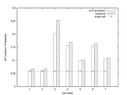
Figure 7: Comparing collision probability $\gamma$ for the example scenario in Figure 3 when each cell contains an AP and $n=5$ STAs. STAs are downloading long files through their respective APs using TCP connections.

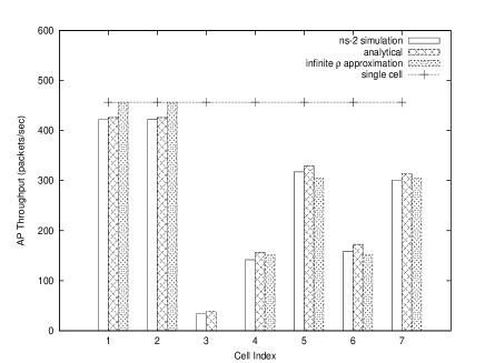
Figure 8: Comparing throughput per node $\theta$ for the example scenario in Figure 3 when each cell contains an AP and $n=5$ STAs. STAs are downloading long files through their respective APs using TCP connections.

O-9.) The collision probability in a WLAN depends, not only on the number of interfering APs but also on the fraction of time for which the neighboring APs can cause collisions. In general, collision probability does not grow as twice the number of interfering APs and depends on the cell topology.

Referring Tables VIII-VIII we extend the validity of the equivalent saturated model of [wanet.bruno08TCPeqvSatModel] as follows:

O-10.) The equivalent saturated model of [wanet.bruno08TCPeqvSatModel] proposed in the context of a single cell, preserves its desirable properties, i.e., it predicts the AP statistics quite well when extended to a multi-cell WLAN that satisfies the PBD condition.

VI-C Variation with $\rho$

Figure 9: Variation of collision probabilities with payload size for the seven cell network in Figure 3 when each cell contains $n=10$ saturated nodes.

Figure 10: Variation of normalized cell throughputs with payload size for the seven cell network in Figure 3 when each cell contains $n=10$ saturated nodes.

Till now, we have discussed the results corresponding to the payload size of 1000 bytes. We now examine how the results vary with the payload size. Figures 10 and 10 depict the variation with payload size of analytically computed collision probabilities and normalized cell throughputs, respectively, for the seven cell network of Figure 3 when each cell contains $n=10$ saturated nodes. Similar results were obtained for the TCP case as well. From Figures 10 and 10, we observe that:

O-11.) The results are largely insensitive to the variation in payload size. Moreover, as the payload size increases, the normalized cell throughputs become closer to the normalized throughputs under the infinite $\rho$ approximation, i.e., they become closer to $x_{1}=x_{2}=1,x_{3}=0,x_{4}=x_{6}=\frac{1}{3},x_{5}=x_{7}=\frac{2}{3}$. Hence, except for very small payload sizes, the infinite $\rho$ approximation can be expected to provide fairly accurate predictions. Furthermore, for sufficiently large payload sizes, we have, $\bar{\Theta}\approx\alpha(\mathcal{G})$.

VII A Simple Design Example

Figure 11: A 12-cell network: Cell indices have been marked. Also shown is the cell level physical contention graph assumed for the network.

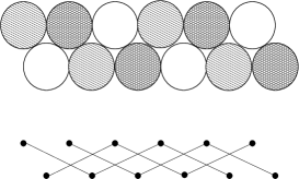
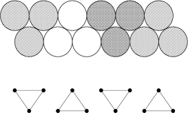
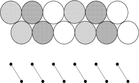
Figure 12: Comparing three channel assignments for a 12-cell network: The cell level logical contention graph are also shown for each assignment.

We consider a 12-cell network as shown in Figure 11 and apply our throughput model to compare three different channel assignments as shown in Figures 12-12. Notice that the “logical” contention graphs for the three assignments in Figures 12-12 are different from the “physical” contention graph of the network shown in Figure 11 which is based on the physical separation among the cells. Two physically dependent cells become logically independent if they are assigned different channels and the corresponding edge will be missing in the logical contention graph. Our objective is to determine the best, among the three assignments, in terms of the normalized network throughput $\bar{\Theta}$ (see Equation 12) and the fairness index reported in [cs.jain_etal84fairness]. Considering fairness at the cell level, the fairness index $J$ is given by [cs.jain_etal84fairness]

$$J:=\displaystyle\frac{(\sum_{i=1}^{N}x_{i})^{2}}{N(\sum_{i=1}^{N}x_{i}^{2})}\;,$$

where we recall that $x_{i}$ is the normalized throughput of Cell-$i$. Note that, $0\leq J\leq 1$, and higher values of $J$ imply more fairness.

Observe that co-channel cells in the first assignment have topology as in Figure 3. There are three subsystem of co-channel cells each consisting of four cells. The infinite $\rho$ approximation predicts that, the two cells at the middle (resp. at the end) for each subsystem of co-channel cells would obtain normalized throughput $\approx\frac{1}{3}$ (resp. $\approx\frac{2}{3}$). The normalized network throughput for the first assignment is $6$ and the fairness index is $0.45$. In the second assignment, each cell obtains normalized throughput $\approx\frac{1}{3}$. The normalized network throughput for the second assignment is $4$ and the fairness index is $1$. Thus, the fairness has attained its maximum in the second assignment. However, this assignment is not desirable since $\bar{\Theta}$ for this assignment is only $\frac{2}{3}$ of $\bar{\Theta}$ in the first assignment. In the third assignment, each cell obtains normalized throughput $\approx\frac{1}{2}$. The normalized network throughput for the third assignment is $6$ and the fairness index is equal to $1$. Clearly, the third assignment is the best one among the three.

Note that, an SINR based model is likely to prefer the first assignment to the third. However, interference by nodes within $R_{cs}$ can be taken care by carrier sensing, and hence, such interference should not be given undue weights. If required, cells that are very close to each other may be assigned the same channel to form “big” cells. Unlike a cell which covers a large area by a single AP and provides connectivity at low PHY rates to STAs that are located at the edge of the cell, a cluster of mutually interfering small co-channel cells each containing an AP to ensure connectivity at high PHY rates can provide high capacity and fairness. This emphasizes the impact of carrier sensing in 802.11 networks.

VIII Applying the Analytical Model along with a Learning Algorithm

In the 12-cell network of Figure 11, with 3 non-overlapping channels, we need to examine $3^{12}$ possibilities to determine the optimal assignment. It is also not clear if the normalized network throughput for the 12-cell network can be actually more than 6 with some other assignment. Under the infinite $\rho$ approximation, the maximum value of $\bar{\Theta}$ is equal to the maximum independence number over all possible logical contention graphs. Clearly, the problem of finding an assignment that maximizes $\bar{\Theta}$ is NP-hard and, in general, it is not desirable to examine all the possibilities.

We now demonstrate how our analytical model could be applied along with a Learning Automata (LA) algorithm called the Linear Reward-Inaction $(L_{R-I})$ algorithm [FAP.sastryetal94LRIgames] to obtain optimal channel assignments. For every cell $i\in\mathcal{N}$, we maintain an $M$-dimensional probability vector $\mbox{\boldmath$p$}_{i}$ where $M$ denotes the number of available channels. The $(L_{R-I})$ algorithm proceeds in steps. Let $k=0,1,2,\ldots$ be the step indices. At each step $k$, a channel is selected for Cell-$i$, $i\in\mathcal{N}$, according to the probability distribution

$$\mbox{\boldmath$p$}_{i}(k):=\Big{(}p_{i,1}(k),p_{i,2}(k),\ldots,p_{i,M}(k)\Big{)},$$

where

$$p_{i,j}(k):=\mbox{ \parbox[t]{190.63338pt}{the probability that Channel-$j$ is selected for Cell-$i$ at step $k$.}}$$

Let $\mbox{\boldmath$c$}(k)=\Big{(}c_{1}(k),c_{2}(k),\ldots,c_{N}(k)\Big{)}$ be the channel assignment at step $k$, where

$$c_{i}(k):=\mbox{the channel selected for Cell-$i$ at step $k$}.$$

Given a channel assignment $c$, we can obtain the logical contention graph $\mathcal{G}(\mbox{\boldmath$c$})$ and applying our throughput model, we can compute the normalized throughput $x_{i}(\mbox{\boldmath$c$})$ of every cell $i$ with the assignment $c$. We define the sum utility for an assignment $c$ by

$$U(\mbox{\boldmath$c$}):=\sum_{i=1}^{N}u(x_{i}(\mbox{\boldmath$c$})),$$ (13)

where $u(\cdot)$ is some suitably defined increasing concave function. For a given $u(\cdot)$, we compute the sum utility at step $k$ by

$$U(\mbox{\boldmath$c$}(k))=\sum_{i=1}^{N}u(x_{i}(\mbox{\boldmath$c$}(k)))\;,$$

and apply the $L_{R-I}$ algorithm which consists of the following steps [FAP.sastryetal94LRIgames]:

1. Begin with $p_{i,j}\in(0,1)$, $\forall i\in\mathcal{N}$, $j=1,2,\ldots,M$, such that $\mbox{\boldmath$p$}_{i}\cdot\mbox{\boldmath$1$}=1$, where $1$ is the $M$-dimensional vector with all components equal to 1.

2. Update the probability vectors of Cell-$i$, $\forall i\in\mathcal{N}$, as

   $$\mbox{\boldmath$p$}_{i}(k+1)=\mbox{\boldmath$p$}_{i}(k)+b\;U(\mbox{\boldmath$c$}(k))\Big{(}\mbox{\boldmath$\delta$}_{c_{i}(k)}-\mbox{\boldmath$p$}_{i}(k)\Big{)}\;,$$

   where $\mbox{\boldmath$\delta$}_{j}$ denotes the $M$-dimensional probability vector with unit mass on Channel-$j$ and $0<b<1$.

The parameter $b$ is called the learning parameter or the step-size parameter which determines the convergence properties of the algorithm; with smaller $b$ convergence is slower but the algorithm may not converge to the desired optimum if $b$ is not small enough [FAP.sastryetal94LRIgames]. Notice that, to ensure non-negativity of the probability vectors after every update with any $b\in(0,1)$, the sum utility $U$ must satisfy $0\leq U\leq 1$. To maximize $\bar{\Theta}=\sum_{i=1}^{N}x_{i}$, we take the average normalized network throughput

$$U_{\bar{\Theta}}:=\displaystyle\frac{1}{N}\sum_{i=1}^{N}x_{i}$$ (14)

as the sum utility $U$ where we compute the $x_{i}$’s applying the infinite $\rho$ approximation. Note that, $0\leq U_{\bar{\Theta}}\leq 1$. Other utility functions can also be considered provided that $0\leq U\leq 1$. Define

$$\mathbf{P}:=(\mbox{\boldmath$p$}_{1},\mbox{\boldmath$p$}_{2},\ldots,\mbox{\boldmath$p$}_{N}).$$

Using the terminology of [FAP.sastryetal94LRIgames], the super vector $\mathbf{P}$ will be called a strategy for the channel assignment problem. A strategy $\mathbf{P}$ such that, $\forall i\in\mathcal{N}$, $p_{i,j}=1$ for some $j$, $j=1,2,\ldots,M$, will be called a pure strategy. A strategy $\mathbf{P}$ that is not a pure strategy is called a mixed strategy. Under the $L_{R-I}$ algorithm, $\{\mathbf{P}(k),k\geq 0\}$ is a Markov process with the pure strategies as the only absorbing states. Thus, in practice, the $L_{R-I}$ algorithm always converges to a pure strategy rather than to a mixed strategy [FAP.sastryetal94LRIgames]. Furthermore, by Theorem 4.1 of [FAP.sastryetal94LRIgames], the $L_{R-I}$ algorithm always converges to one of the Nash equilibria. Thus, in practice, channel assignment by the $L_{R-I}$ algorithm always provides an assignment $\mbox{\boldmath$c$}^{*}$ which is one of the Nash equilibria in pure strategies in the sense that

$$U(\mbox{\boldmath$c$}^{*})\geq U(\mbox{\boldmath$c$}),$$

for all $c$ that differs from $\mbox{\boldmath$c$}^{*}$ by exactly one element, i.e., changing the channel of one of the cells in the assignment $\mbox{\boldmath$c$}^{*}$ does not increase the sum utility $U$.

VIII-A Results for Channel Assignment by the $L_{R-I}$ Algorithm

Figure 13: Evolution of the average normalized network throughput $U_{\bar{\Theta}}$ under the $L_{R-I}$ algorithm for the 12-cell network in Figure 11 with $M=3$ channels, $b=0.01$, and $p_{ij}=\frac{1}{3}$, $\forall i\in\mathcal{N}$ and $j=1,2,\ldots,M$.

Figure 14: Evolution of the average normalized network throughput $U_{\bar{\Theta}}$ for the 7-cell example in Figure 3 with $M=2$ channels, $b=0.01$, and $p_{i1}=p_{i2}=0.5$, $i=1,2,\ldots,7$. In this example, the $L_{R-I}$ algorithm converges to a global optimum.

Figure 15: Evolution of the average normalized network throughput $U_{\bar{\Theta}}$ for the 7-cell example in Figure 3 with $M=2$ channels, $b=0.01$, and $p_{i1}=p_{i2}=0.5$, $i=1,2,\ldots,7$. In this example, the $L_{R-I}$ algorithm converges to a local optimum.

Figure 13 shows the evolution of the average normalized network throughput $U_{\bar{\Theta}}$ under the $L_{R-I}$ algorithm with $M=3$ channels and $b=0.01$ for the 12-cell network in Figure 11. We began with uniform unbiased probability vectors $\mbox{\boldmath$p$}_{i}=(\frac{1}{3},\frac{1}{3},\frac{1}{3})$, $\forall i\in\mathcal{N}$. The algorithm converged to the assignment $c_{1}=c_{6}=c_{9}=1,{c_{4}=c_{7}=c_{12}=3},c_{2}=c_{3}=c_{5}=c_{8}=c_{10}=c_{11}=2$. Notice that $U_{\bar{\Theta}}$ converges to $\frac{2}{3}$ which corresponds to $\bar{\Theta}=8$. It can be verified that this is the maximum possible value that $\bar{\Theta}$ can take for the given network with 3 channels. We found that the $L_{R-I}$ algorithm always converges to a globally optimum solution if started with uniform unbiased probability vectors and if $b$ is sufficiently small. However, starting with probability vectors that are highly biased towards some assignment or if $b$ is not small enough, it may not converge to a globally optimum solution. We demonstrate this through Figures 15-17 for the 7-cell example in Figure 3 with $M=2$ channels.

Figure 16: Evolution of the average normalized network throughput $U_{\bar{\Theta}}$ for the 7-cell example in Figure 3 with $M=2$ channels, $b=0.001$, and $p_{11}=p_{21}=p_{32}=p_{42}=p_{51}=p_{61}=p_{72}=0.8$. In this example, the $L_{R-I}$ algorithm converges to a global optimum.

Figure 17: Evolution of the average normalized network throughput $U_{\bar{\Theta}}$ for the 7-cell example in Figure 3 with $M=2$ channels, $b=0.001$, and $p_{11}=p_{21}=p_{32}=p_{42}=p_{51}=p_{61}=p_{72}=0.9$. In this example, the $L_{R-I}$ algorithm converges to a local optimum.

Beginning with unbiased probability vectors and $b=0.01$ the algorithm may converge to a global optimum with $U_{\bar{\Theta}}=1$ or $\bar{\Theta}=7$ (Figure 15). There are two possible global optima, namely, $c_{1}=c_{2}=c_{4}=c_{7}=1,c_{3}=c_{5}=c_{6}=2$ and $c_{1}=c_{2}=c_{4}=c_{7}=2,c_{3}=c_{5}=c_{6}=1$. In Figure 15, we show that, with $b=0.01$, the algorithm may also converge to a solution that is not a global optimum. In fact, for the specific simulation run, the algorithm converged to the Nash equilibrium $c_{1}=c_{2}=c_{5}=c_{6}=1,c_{3}=c_{4}=c_{7}=2$ with $\bar{\Theta}=6$ which is not a global optimum. The assignment $c_{1}=c_{2}=c_{5}=c_{6}=1,c_{3}=c_{4}=c_{7}=2$ is a Nash equilibrium in the sense that changing the channel of one of the cells does not increase $\bar{\Theta}$, and hence, the sum utility $U_{\bar{\Theta}}$. With $b=0.001$, and beginning with unbiased uniform probability vectors, we observed that the algorithm always converged to a global optimum. With $b=0.001$, the algorithm converged to a global optimum even when we began with probability vectors biased towards the assignment $c_{1}=c_{2}=c_{5}=c_{6}=1,c_{3}=c_{4}=c_{7}=2$ (Figure 17). However, when the initial probability vectors were highly biased towards the assignment $c_{1}=c_{2}=c_{5}=c_{6}=1,c_{3}=c_{4}=c_{7}=2$, the algorithm converged to the biased assignment which is not a global optimum (Figure 17).

IX A Simple and Fast Algorithm for Maximizing Normalized Network Throughput

We observe that the $L_{R-I}$ algorithm takes a large number of iterations to converge and guarantees convergence only to Nash equilibria. Clearly, for the 7-cell example with $M=2$ channels, an exhaustive search would have required examination of only $2^{7}=128$ possibilities whereas the $L_{R-I}$ algorithm takes many more steps to converge. The Linear Reward-Penalty ($L_{R-P}$) algorithm of [wanet.leith_clifford06CFL] and the simulated annealing algorithm of [wanet.kauffmann07selfOrganization] guarantee convergence to a globally optimum solution as the number of iterations goes to infinity. A greedy version of simulated annealing algorithm in [wanet.kauffmann07selfOrganization] is relatively faster but still takes a large number of iterations to converge and guarantees convergence only to locally optimum solutions. To maximize the normalized network throughput $\bar{\Theta}$ we now propose a simple and fast decentralized algorithm which can be easily implemented in real networks.

We form a physical contention graph $\mathcal{G}$ in which every completely dependent pair of cells are neighbors (since we have not yet assigned channels) and our objective is to transform $\mathcal{G}$ to a logical contention graph $\mathcal{G}(\mbox{\boldmath$c$})$ by an assignment $c$ so that $\alpha(\mathcal{G}(\mbox{\boldmath$c$}))$ is maximized. As noted in Observation O.11, for sufficiently large packet sizes, we have $\bar{\Theta}\approx\alpha(\mathcal{G})$. Hence, maximizing $\alpha(\mathcal{G}(\mbox{\boldmath$c$}))$ would maximize $\bar{\Theta}$.

Maximal Independent Set Algorithm (mISA) : We propose the following channel assignment algorithm: (recall that $M$ is the number of available channels)

(1) Choose a maximal independent set (mIS) of cells, assign them Channel-1 and remove them from the graph.

(2) Increment the channel index and repeat the procedure on the residual graph until one channel is left.

(3) Assign Channel-$M$ to all the cells in the residual graph after $M-1$ steps.

Notice that mISA takes only $M$ steps. Also notice that, the residual graph may become null (i.e., it might not have any vertices left) after $M^{\prime}<M$ steps. Clearly, mISA is based on a classical graph coloring technique, but the novelty lies in our recognition of the notion of optimality that mISA provides which is given by the following

Theorem IX.1

The channel assignments by mISA are Nash equilibria in pure strategies for the objective of maximizing normalized network throughput $\bar{\Theta}$ as $\rho_{i}\rightarrow\infty$, $\forall i\in\mathcal{N}$. Furthermore, mISA provides a globally optimum solution if $M\geq D(\mathcal{G})+1$ where $D(\mathcal{G})$ denotes the maximum vertex degree in the physical contention graph $\mathcal{G}$.