Nanostratification of optical excitation in self-interacting 1D arrays

Abstract

The major assumption of the Lorentz–Lorenz theory about uniformity of local fields and atomic polarization in dense material does not hold in finite groups of atoms, as we reported earlier [A. E. Kaplan and S. N. Volkov, Phys. Rev. Lett. 101, 133902 (2008)]. The uniformity is broken at sub-wavelength scale, where the system may exhibit strong stratification of local field and dipole polarization, with the strata period being much shorter than the incident wavelength. In this paper, we further develop and advance that theory for the most fundamental case of one-dimensional arrays, and study nanoscale excitation of so called “locsitons” and their standing waves (strata) that result in size-related resonances and related large field enhancement in finite arrays of atoms. The locsitons may have a whole spectrum of spatial frequencies, ranging from long waves, to an extent reminiscent of ferromagnetic domains, – to super-short waves, with neighboring atoms alternating their polarizations, which are reminiscent of antiferromagnetic spin patterns. Of great interest is the new kind of “hybrid” modes of excitation, greatly departing from any magnetic analogies. We also study differences between Ising-like near-neighbor approximation and the case where each atom interacts with all other atoms in the array. We find an infinite number of “exponential eigenmodes” in the lossless system in the latter case. At certain “magic” numbers of atoms in the array, the system may exhibit self-induced (but linear in the field) cancellation of resonant local-field suppression. We also studied nonlinear modes of locsitons and found optical bistability and hysteresis in an infinite array for the simplest modes.

This paper is now published, with very minor changes, in Phys. Rev. A 79, 053834 (2009).

I Introduction

This paper is a theoretical extension of our recent Letter cit1 on nanoscale stratification of local field and atomic dipole excitation in low-dimensional lattices driven by a laser at the frequency of the resonant atomic transition. We focus here on the most fundamental case of a one-dimensional (1D) array of resonant atoms, and construct a detailed theory of both linear and nonlinear interactions in the system, resulting in such phenomena as sub-wavelength spatial modulation (stratification) of polarization and local field, long-wave and short-wave stratification, size-related resonances and large field enhancement, “magic” numbers, ferromagnetic- and antiferromagneticlike atomic polarization, optical bistability and hysteresises, etc. In addition to the results cit1 and their derivations, we also present new results (i) on the size-related resonances using a many-body approximation involving interactions of each atom with all other atoms in the array, beyond the Ising-like approximation whereby atoms only interact with their nearest neighbors, (ii) on traveling locsiton waves and their dissipation, as well as an estimate of the maximum size of the 1D array to support most of the effects discussed here, (iii) on hysteresises and optical bistability in arbitrarily long arrays, and (iv) general mathematical consideration of dispersion relation in the self-interacting arrays for dipole approximation and beyond it.

It is well known that optical properties of sufficiently dense materials are substantially affected by the near-field interactions between neighboring particles at the frequency of the incident field, in particular, quasi-static (non-radiative) dipole interactions. The best known manifestation of this fact is the local vs incident field phenomenon and related Lorentz–Lorenz or Clausius–Mossotti relations cit2 for dielectric constant as a nonlinear function of the number density. The microscopic (or local) field (LF), $\mathbf{E}_{\mathrm{L}}$, acting upon atoms or molecules becomes then different from both the applied and average macroscopic fields because of inter-particle interaction. In the most basic case, that relation between $\mathbf{E}_{\mathrm{L}}$ and the average field $\mathbf{E}$ is $\mathbf{E}_{\mathrm{L}}=(\epsilon+2)\mathbf{E}/3$, where $\epsilon$ is the dielectric constant of the material at the laser frequency $\omega$. It is worth noting that we are not interested here in the relation between $\epsilon$ and the number density of the material, since in the case of small 1D or 2D arrays the issue is moot. For the same reason, it also makes sense to deal directly with the incident field, $\mathbf{E}_{\mathrm{in}}$, instead of the averaged field. In most theories of those interactions a traditional standard (and at that often implicit) assumption, reflected also in the above formula, is that the local field and polarization are uniform in the near neighborhood of each particle at least at the distances shorter than the wavelength of light, $\lambda$. This essentially amounts to the so called “mean-field approximation”.

It was shown by us cit1 , however, that if the local uniformity is not presumed, then, under certain conditions on the particle density and their dipole strengths, the system of interacting particles is bound to exhibit periodic spatial variations of polarization and local-field amplitude. These variations result in sub-wavelength strata with a nanoscale period much shorter than $\lambda$. Under certain conditions, the system may exhibit an ultimate non-uniformity, whereby each pair of neighboring atoms in 1D arrays has their dipoles counter-oscillating with respect to each other, i. e. their excitations and thus local fields have opposite signs.

To a certain extent this is reminiscent of the situation in magnetic materials with ferromagnetic vs antiferromagnetic effects. Indeed, the mean-field approximation which is at the root of the Curie–Weiss theory of ferromagnetism cit3 , is based on the assumption of uniform polarization of all the neighboring magnetic dipoles even without external magnetic field, when taking into account their interaction with each other. Contrary to that, the Ising theory cit3 , which does not make the assumption of uniformity, showed that even in the near-neighbor approximation for that interaction, the excitation may result in counter-polarization of neighboring atoms in 1D arrays, and thus in a new phenomenon of antiferromagnetism. Note here that in these effects there is no notion of “local” vs “external” field phenomenon: in a “pure” case of either of the magnetic effects, no external field is applied; the effects here are the result of self-organization of permanent, “hard”, atomic dipoles with pre-existing dc dipole fields, without any “help from outside”.

In this lies a profound difference between dc magnetic material phenomena (ferro- and antiferromagnetism) on the one hand – and the effects considered by us here and in cit1 on the other hand, all of which are based on the optical (or, in general, any other quantum or classical resonance) excitation of atoms (or other small particles, e. g. quantum dots, clusters, small-particle plasmons, etc.). While magnetic dipoles in ferromagnetics are nonzero even in the absence of an external field (we may call them “hard” dipoles), the oscillating dipoles (in the linear case) can be induced only by the driving field at the near-resonant frequency, so they can be called “soft” dipoles; without such a driving their polarization vanishes. Because in dense material the atoms actually are acted upon by local field, the response of each one of them may differ from the others by phase and amplitude (or even direction), with some of the dipoles fully suppressed while others fully excited. Thus the effects considered here are induced by the interplay of external and local fields, which put the entire phenomenon squarely into the domain of relations between the local and incident fields. Because of that, since the phenomenon depends strongly on the characteristics of the incident field (polarization, frequency, and, in the nonlinear case, intensity), the spatial modulation of the dipole excitation and local field can vary substantially. This results in a wealth of different patterns, some of them reminiscent of the ferromagnetic, other of antiferromagnetic, but the most of them forming all kinds of hybrid patterns. The complete cross-over from ferromagneticlike to antiferromagneticlike state of the system with all the intermediate states can be attained then by simply tuning laser frequency.

Another significant difference here is that the system size is small. Provided there is sufficiently strong interparticle interaction, the new phenomenon can occur in the vicinity of boundaries, lattice defects, impurities or in sufficiently small group of atoms; recent advances in technology allow fabrication of nanoscale structures with small numbers of atoms. Thus, our theory emphasizes phenomena in relatively small ordered arrays of interacting atoms, in contrast to, e. g., microscopic models of ferromagnetism that mostly focus on averaged, “thermodynamic” perspective on sufficiently large systems. This brings forward a new set of nanoscale phenomena. Harking back to ferromagnetic systems, this new emphasis may reveal similar phenomena for nanoscale magnetic systems, which could be an exciting topic for a separate study.

Our choice of 1D and 2D dielectric systems based on the arrays or lattices of atoms, quantum dots, clusters, molecules, etc., allows to control anisotropy of near-field interaction. It also eliminates the issues of electromagnetic (EM) propagation being modified by the effects as the EM wave propagates through the structure (especially if it propagates normally to the lattice).

If local uniformity is broken by any perturbation, the system may exhibit near-periodic spatial sub-$\lambda$ patterns (strata) of polarization. In general, two major modes of the strata transpire: short-wave (SW), with the period up to four interatomic spacings, $l_{a}$, and long-wave (LW) strata. The strata are standing waves of elementary LF excitations (called locsitons in cit1 ) having a near-field, electrostatic, nature and low group velocity.

In the first approximation, the phenomenon is linear in the driving field, and the locsitons may be excited within a spectral band much broader than the atomic linewidth. It can be viewed as a Rabi broadening of an atomic line by interatomic interactions. The strata are controlled by laser polarization and the strength of atom coupling, $Q$, via atomic density, dipole moments, relaxation, and detuning. Once $|Q|>Q_{\mathrm{cr}}=O(1)$, the LF uniformity can be broken by boundaries, impurities, vacancies in the lattice, etc. A striking manifestation of the effect is large field resonances due to locsiton eigenmodes in finite lattices, and – at certain, “magic” numbers of atoms in the lattice – almost complete cancellation of field suppression at the atomic resonance; saturation nonlinearity results in hysteresises and optical bistability.

The paper is structured as follows. In Section II we derive the main equations for self-interacting atomic lattices of arbitrary dimensions using two-level (nonlinear in general) model for atomic resonances and dipole–dipole interaction between atoms, while Section III is on specific equations for linear infinite and finite 1D arrays. In Section IV we develop the general theory of locsitons and derive the dispersion relation. In Section V we study locsiton band formation, size-related resonances due to standing waves of locsitons (strata) and local-field enhancement. In Section VI we concentrate on detailed theory of resonances beyond the near-neighbor approximation, including evanescent solutions (see also Section IV). Magic numbers are considered in Section VII. In Section VIII, we study the effects of losses on locsiton excitation, depth of penetration, and traveling locsiton waves. Section IX is on nonlinear locsiton modes, in particular, optical bistability and hysteresis. Section X addresses potential applications of locsitons and their analogies in other physical systems. In Conclusions, Section XI, we summarize our results. Appendix A is on general mathematical aspects of dispersion relations for 1D arrays.

II Main equations

Our model is based on the near-field dipole atomic interactions, with the incident frequency $\omega$ being nearly resonant to an atomic transition with a dipole moment $\mathbf{d}_{a}$ at the frequency $\omega_{0}$. In the linear case, i. e. when the laser intensity is significantly lower than that for the quantum transition saturation (see below), the result of this model coincides with that of a classical harmonic oscillator formed by an electron in a harmonic potential with the same resonant frequency $\omega_{0}$ and with the dipole moment

$$|d_{a}|=\frac{e}{2\pi}\sqrt{\lambda_{\mathrm{C}}\lambda/2},$$ (1)

where $\lambda_{\mathrm{C}}=2\pi\hbar/mc$ is the Compton wavelength of electron.

In a standard LF situation, $\lambda\gg l_{a}$, where $\lambda=2\pi c/\omega$, the field of an elementary dipole with the polarization $\mathbf{p}$ is dominated in its near vicinity by a non-radiative, quasi-static (and only electric) component, which is strongly anisotropic in space. This dominant term in the near-field area, $|\mathbf{r}^{\prime}-\mathbf{r}|=r_{0}\ll\lambda$, attenuates as $1/r_{0}^{3}$ (see e. g. cit4 , Section 72). At $|d_{a}|\ll r_{0}\ll\lambda$ the amplitude of the field of an oscillating dipole located at $\mathbf{r}^{\prime}$ induces a field at the point of observation $\mathbf{r}$ with the amplitude coinciding with that of an elementary static dipole with the same polarization $\mathbf{p}^{\prime}$:

$$\mathbf{E}_{\mathrm{dp}}(\mathbf{r}^{\prime},\mathbf{r})=\frac{3\mathbf{u}(\mathbf{p}^{\prime}\cdot\mathbf{u})-\mathbf{p}^{\prime}}{\epsilon|\mathbf{r}^{\prime}-\mathbf{r}|^{3}},$$ (2)

where $\mathbf{u}=(\mathbf{r}-\mathbf{r}^{\prime})/r_{0}$ is a unit vector in the direction of observation, and $\epsilon$ is a background dielectric constant.

We will model a resonant atomic transition by a basic two-level atom in a steady-state mode under the action of a field, $\mathbf{E}\exp(-i\omega t)/2+\mathrm{c.c.}$, with the amplitude $\mathbf{E}$ and frequency $\omega$, and assume that $l_{a}\gg|d_{a}|/e$, so that the wave functions of neighboring atoms do not overlap. Using a semi-classical approach standard in LF theory of resonant atoms cit5 ; cit6 , we can now find the atomic polarization as:

$$\mathbf{p}=-\frac{2|d_{a}|^{2}}{\hbar\Gamma}\frac{\mathbf{E}\Delta N}{\delta+i},$$ (3)

where $\mathbf{p}$ is the polarization amplitude [the full polarization is then $\mathbf{p}\exp(-i\omega t)/2+\mathrm{c.c.}$]; $\Delta N=N_{1}-N_{2}$ is the population difference, with $N_{1}$ and $N_{2}$ being atomic populations at respective ground and excited levels ($N_{1}+N_{2}=1$),  $\delta=T\Delta\omega=T(\omega-\omega_{0})$ is a dimensionless detuning from the resonant frequency $\omega_{0}$ of the two-level atom, $T=2/\Gamma$ is a transverse relaxation time (the time of polarization relaxation) and $\Gamma$ is the (homogeneous) linewidth of the linear resonance . In turn, the steady-state population difference is cit5

$$\Delta N=N^{\mathrm{eq}}\left(1+T\tau\frac{|d_{a}E/\hbar|^{2}}{1+\delta^{2}}\right)^{-1},$$ (4)

where $\tau$ is a longitudinal relaxation time (life-time of the excited atom), and $N^{\mathrm{eq}}$ is an equilibrium population difference at the system temperature due to Boltzmann’s distribution; in optics one can usually assume $N^{\mathrm{eq}}\approx 1$, so that

$$\Delta N \approx \left[1+\frac{|E|^{2}/E_{\mathrm{sat}}^{2}}{1+\delta^{2}}\right]^{-1}\equiv f_{\mathrm{NL}}(|E|^{2}),$$

$$E_{\mathrm{sat}}^{2} = \frac{\hbar^{2}}{|d_{a}|^{2}}\cdot\frac{1}{\tau T},$$ (5)

where $E_{\mathrm{sat}}^{2}$ is the saturation intensity, and $f_{\mathrm{NL}}(|E|^{2})$ is nonlinearity due to saturation. Substituting (5) into (3), one obtains a closed-form expression for the polarization,

$$\mathbf{p}=-\mathbf{E}\frac{2|d_{a}|^{2}}{\hbar\Gamma(\delta+i)}f_{\mathrm{NL}}(|E|^{2}).$$ (6)

For a classical harmonic (linear) oscillator we have:

$$\mathbf{p}=-\frac{\mathbf{E}e^{2}}{\omega_{0}\Gamma m(\delta+i)},$$ (7)

where $m$ is the mass of electron.

The local field $\mathbf{E}_{\mathrm{L}}(\mathbf{r})$ at each atom is the incident laser field, $\mathbf{E}_{\mathrm{in}}$, plus the sum of the near-fields, $\mathbf{E}_{\mathrm{dp}}(\mathbf{r}^{\prime},\mathbf{r})$ (2), induced by all the surrounding dipoles at $\mathbf{r}^{\prime}$ acted upon by the respective local fields $\mathbf{E}_{\mathrm{L}}(\mathbf{r}^{\prime})$, i. e.

$$\mathbf{E}_{\mathrm{L}}(\mathbf{r}) = \mathbf{E}_{\mathrm{in}}(\mathbf{r})+\sum_{\mathrm{latt}}^{\mathbf{r}^{\prime}\neq\mathbf{r}}\mathbf{E}_{\mathrm{dp}}(\mathbf{r}^{\prime},\mathbf{r})$$ (8)

$$= \mathbf{E}_{\mathrm{in}}(\mathbf{r})+\frac{1}{\epsilon}\sum_{\mathrm{latt}}^{\mathbf{r}^{\prime}\neq\mathbf{r}}\frac{3\mathbf{u}(\mathbf{p}^{\prime}\cdot\mathbf{u})-\mathbf{p}^{\prime}}{|\mathbf{r}^{\prime}-\mathbf{r}|^{3}},$$

where $\sum_{\mathrm{latt}}$ denotes summation over the entire lattice or array. To obtain a closed-form master equation, e. g. for $\mathbf{E}_{\mathrm{L}}(\mathbf{r})$ alone, we use (6) to write:

$$\mathbf{E}_{\mathrm{L}}(\mathbf{r})=\mathbf{E}_{\mathrm{in}}(\mathbf{r})-\frac{Q}{4}\sum_{\mathrm{latt}}^{\mathbf{r}^{\prime}\neq\mathbf{r}}\left|\frac{l_{a}}{\mathbf{r}^{\prime}-\mathbf{r}}\right|^{3}$$

$$\quad{}\times\left\{3\mathbf{u}[\mathbf{E}_{\mathrm{L}}(\mathbf{r}^{\prime})\cdot\mathbf{u}]-\mathbf{E}_{\mathrm{L}}(\mathbf{r}^{\prime})\right\}f_{\mathrm{NL}}[|\mathbf{E}_{\mathrm{L}}(\mathbf{r}^{\prime})|^{2}],$$ (9)

where $\mathbf{E}_{\mathrm{L}}(\mathbf{r})$ are local fields only at the locations of atoms in the lattice and not at any other points inside or outside it; $Q=Q_{a}/(\delta+i)$ is a tuning-dependent strength of dipole–dipole interaction, and the maximum absolute strength, $Q_{a}$, is

$$Q_{a}=\frac{8|d_{a}|^{2}}{\epsilon\hbar\Gamma l_{a}^{3}}=\frac{4\alpha}{\pi\epsilon}\frac{\lambda_{0}(|d_{a}|/e)^{2}}{l_{a}^{3}}\frac{\omega_{0}}{\Gamma},$$ (10)

where $\alpha=e^{2}/\hbar c\approx 1/137$ is the fine-structure constant, and nonlinear factor $f_{\mathrm{NL}}$ is as in (5). For a classical harmonic oscillator, (1), we have

$$(Q_{a})_{\mathrm{class}}=\frac{4e^{2}}{\epsilon m\omega_{0}\Gamma l_{a}^{3}}=\frac{1}{\epsilon\pi^{2}}\frac{r_{e}\lambda_{0}^{2}}{l_{a}^{3}}\frac{\omega_{0}}{\Gamma},$$ (11)

where $r_{e}\equiv e^{2}/m_{e}c^{2}\approx 2.8\times 10^{-6}$ nm is the classical radius of electron.

Eqs. (8), (9) reflect many-body nature of the interaction. A conventional approach to local fields within the Lorentz–Lorenz theory is to look for a self-consistent solution for the fields in this interaction, with an assumption, however, that they are uniform (the mean-field theory), i. e. to set $\mathbf{E}_{\mathrm{L}}(\mathbf{r})=\mathbf{E}_{\mathrm{L}}(\mathbf{r}^{\prime})$ and also use an encapsulating sphere around the observation point. These assumptions effectively shut out any strong spatial variations of the atomic excitations and local field that may exist at the inter-atomic scale. That is where we depart from the Lorentz–Lorenz theory; none of those assumptions are used here, and our approach is to use general expressions (8) or (9) and seek straightforward solution for them.

We will see below that the major critical condition for the phenomenon to exist and be observable at least at other optimal conditions is that $Q_{a}$ exceeds some critical value, $Q_{a}>O(1)$. Three parameters are critical in this respect: atomic dipole moment $d_{a}$, the spacing between atoms, $l_{a}$, and the atomic linewidth, $\Gamma$, since $Q_{a}\propto|d_{a}|^{2}/(\Gamma l_{a}^{3})$. To get an idea of whether the above critical condition is realistic, let us look first at the case of a gas-like collection of atoms, with the relaxed requirement on the spacing $l_{a}$. Large dipole moments and narrow resonances in, e. g., alkali vapors cit6 or CO₂ gas cit5 , in solids cit8 , quantum wells and clusters may greatly enhance the phenomenon and allow for $l_{a}$ from sub-nanometer to a few tens of nanometers. Considering an example with $l_{a}\sim 100$ Å, corresponding to the volume density of $\sim 10^{18}$ cm^-3, $|d_{a}|/e\sim 1$ Å,  $\lambda_{0}\sim 1$ $\mu\mathrm{m}$, $\epsilon=1$, and $\Gamma/\omega_{0}\sim 10^{-6}$, all of which are reasonable data, we obtain $Q_{a}\sim 10^{2}$, which provides a margin large enough to see all the effects discussed here. It is also of interest to roughly estimate what is the upper limit for $Q_{a}$. To that end, consider the extreme situation of $l_{a}\sim|d_{a}|/e$ (solid-state- or liquid-like packing of participating atoms), in which case we have the ceiling for $Q_{a}$ as

$$Q_{\mathrm{ceil}}=\frac{8e^{3}}{\epsilon\hbar\Gamma|d_{a}|}=\frac{4\alpha}{\pi\epsilon}\frac{\lambda_{0}}{(|d_{a}|/e)}\frac{\omega_{0}}{\Gamma}.$$ (12)

Even taking into consideration significant line broadening, $\Gamma$, $Q_{\mathrm{ceil}}$ may exceed unity by many order of magnitude, thus providing huge margin for the existence and observation of locsitons and related effects.

III 1D array of atoms: linear case

We consider here the most basic model of a 1D array of $N$ atoms lined up along the $z$ axis, spaced by $l_{a}$, and driven by a laser propagating normally to the array and having an arbitrary polarization (Fig. 1).

Figure 1: 1D array of atoms and laser light with different polarizations; light is incident normally to the plane of the graph.

In the linear case, $|E_{\mathrm{L}}|^{2}\ll E_{\mathrm{sat}}^{2}$, when in (9) $f_{\mathrm{NL}}=1$, it is sufficient to consider effects caused by linearly polarized light with either one of the two mutually orthogonal polarizations; any other polarization (e. g. a circular one) can be treated as a linear combination of those two. In the case of a 1D array, natural choices for these two basic configurations are:

• the incident field $\mathbf{E}_{\mathrm{in}}$ is parallel to the $z$ axis, $\mathbf{E}_{\mathrm{in}}\parallel\hat{\mathbf{e}}_{z}$ (and the dipoles line up “head-to-tail”; we will call it $\parallel$-configuration), and

• $\mathbf{E}_{\mathrm{in}}$ is normal to the $z$ axis, $\mathbf{E}_{\mathrm{in}}\perp\hat{\mathbf{e}}_{z}$ (“side-by-side” lineup; $\perp$-configuration).

The general solution will be a linear vectorial superposition of these two. This choice of the basic configurations is dictated by the simplicity of the resulting polarization of the local field. Indeed, in both cases, it follows that the polarization of local field is parallel to that of the incident field, $\mathbf{E}_{\mathrm{L}}\parallel\mathbf{E}_{\mathrm{in}}$, so we can use scalar equations for all fields. Using the dimensionless notation $\mathbf{\mathcal{E}}_{n}=[E_{\mathrm{L}}(\mathbf{r}_{n})/E_{\mathrm{in}}]_{(p)}$, where $(p)$ denotes polarization, $(p)=\>\parallel$ or $(p)=\>\perp$, and recalling that now $\mathbf{u}\parallel\hat{\mathbf{e}}_{z}$, we write (9) for both configuration as

$$\mathcal{E}_{n}+QF_{(p)}\sum_{1\leq j\leq N}^{j\neq n}\frac{\mathcal{E}_{j}/2}{|j-n|^{3}}=1,\quad\mbox{if}\quad n=1,\ldots,N,$$

$$\mbox{and}\quad\mathcal{E}_{n}=0\quad\mbox{otherwise},$$ (13)

where $F_{(p)}$ is a form-factor due to polarization configuration: $F_{\parallel}=1$ and $F_{\perp}=-1/2$.

If the 1D array is infinite, $N\to\infty$, or sufficiently long, $N\gg 1$, it is instructive to rewrite (13) in the form

$$\mathcal{E}_{n}+SQF_{(p)}\sum_{-\infty\leq j\leq\infty}^{j\neq n}\frac{\mathcal{E}_{j}/2S}{|j-n|^{3}}=1,$$ (14)

where $S=\sum_{j=1}^{\infty}j^{-3}\approx 1.202057$. The sums over $|j-n|^{-3}$ in (13), (14) converge rather fast, hence $S-1$ is not too large, see also Appendix A below. Eqs. (13) and (14), the same as master equation (9), represent the case of fully-interacting arrays (FIA), whereby each atom “talks” to all the other atoms in the array, which presents a challenge to an analytical treatment. Of course, a linear equation (13) for $\mathcal{E}_{n}$ is solved analytically using a standard linear algebra approach with matrices. However, analyzing the results for large-size arrays, $N\gg 1$, in particular analytically finding all the resonances in $(\mathcal{E}_{n})_{\mathrm{max}}(\delta)$, can only be done by using numerical matrix solver, even if we neglect the dissipation.

Thus, there is a need for a simple approximation that would preserve most of the qualitative features of the phenomenon, yet could be easily analyzed analytically. This can be done by using the near-neighbor approximation (NNA), similar to that of the Ising model of (anti)ferromagnetism, in which the full sum in (13) or (14) is replaced by the sum over the nearest neighbors,

$$\mathcal{E}_{n}+\frac{QF_{(p)}}{2}(\mathcal{E}_{n-1}+\mathcal{E}_{n+1})=1,$$

$$\mathcal{E}_{0}=\mathcal{E}_{N+1}=0.$$ (15)

In the ultimate two-atom case, $N=2$ cit1 , the two approaches merge. The further two-near-neighbors approximation (2-NNA) and even three-near-neighbors approximation are considered in Section VI below. We found, however, that in general, a full summation (FIA) in (13) on the one hand, and NNA (15) as well as 2-NNA on the other hand, produce qualitatively similar results that differ by a factor of $O(1)$.

Since effects discussed here are most pronounced in relatively small systems or in the small vicinity of perturbations in large lattices, it is natural to stipulate that the incident field within the array is uniform, unless otherwise is stated; however, this condition can readily be arranged even for an array larger than $\lambda$. One of the solutions for the local field (and atomic excitation) in the infinite 1D array (or a sufficiently long one, whereby we can neglect edge effects) is also uniform. We will call it the “Lorentz” solution, $\bar{\mathcal{E}}$, to be found from (14) by setting $\mathcal{E}_{n}=\mathcal{E}_{j}=\bar{\mathcal{E}}$ as:

$$\bar{\mathcal{E}}_{(p)}=\frac{1}{1+QSF_{(p)}}=\frac{1}{1-[(\delta_{\mathrm{LL}})_{(p)}/(\delta+i)]},$$

$$(\delta_{\mathrm{LL}})_{(p)}=-SQ_{a}F_{(p)},$$ (16)

where we introduced polarization-dependent parameter $\delta_{\mathrm{LL}}$, which determines Lorentz–Lorenz shift at $\delta=\delta_{\mathrm{LL}}$ (see below); $|\delta_{\mathrm{LL}}|$ is a measure of the polarization-related strength of interaction. Eq. (16) may be viewed as a 1D counterpart of the Lorentz–Lorenz relation for local field; notice, however, that the field $\bar{\mathcal{E}}$ is strongly anisotropic with respect to the polarization. The spectral behavior of $|\bar{\mathcal{E}}|$ is depicted in Fig. 2 with thicker dashed curves in all the graphs.

Figure 2: Spectra of absolute maximum local field amplitudes near an atomic resonance ($\delta=0$) in the near-neighbor approximation with $\delta_{\mathrm{LL}}=200$: (a) locsiton resonances with 12 atoms in the array; (b) the same with 13 (magic number) atoms in the array; (c) merging and damping of locsiton resonances for a large number of atoms, $N=100$. The curves show the amplitudes of local fields for size-related resonances, local fields due to Lorentz–Lorenz theory, and lower and upper amplitude envelopes of the resonances.

If $Q_{a}\gg 1$, it shows, as one may expect, a deep dip at the atomic resonance frequency, i. e. at $\delta=0$,

$$|\bar{\mathcal{E}}_{(p)}|_{\mathrm{min}}^{2}=\frac{1}{1+\delta_{\mathrm{LL}}^{2}}$$ (17)

(so that at the atomic resonance the local field is suppressed, as if it is pushed out of the array), and a strong new resonant peak appears at the shifted frequency $\delta=\delta_{\mathrm{LL}}$ due to the Lorentz–Lorenz effect:

$$|\bar{\mathcal{E}}_{(p)}|_{\mathrm{max}}^{2}=1+\delta_{\mathrm{LL}}^{2}=\frac{1}{|\bar{\mathcal{E}}_{(p)}|_{\mathrm{min}}^{2}},$$ (18)

whose nature is essentially similar to e. g. Lorentz–Lorenz resonance observed experimentally in alkali vapors cit6 . However, in the 1D case considered here, the Lorentz–Lorenz shift and even its sign are polarization-dependent; in particular,

$$(\delta_{\mathrm{LL}})_{\parallel}=-Q_{a}S,\qquad(\delta_{\mathrm{LL}})_{\perp}=Q_{a}S/2,$$ (19)

i. e. the Lorentz–Lorenz resonance is red-shifted for $\parallel$-polarization of laser, and blue-shifted for $\perp$-polarization. The Lorentz field $\bar{\mathcal{E}}$ and Lorentz–Lorenz shift in the near-neighbor approximation, Eq. (15), are determined by the same equations (16)–(19), where one has to set $S=1$.

IV Spatially-periodic and wave solutions (locsitons)

We look now for solution of Eq. (14) as the sum of uniform LF, $\bar{\mathcal{E}}$, Eq. (16), and oscillating ansatz $\Delta\mathcal{E}\propto\exp(\pm iqn)$, where $q$ is an (unknown) wavenumber, similarly, e. g. to the phonon theory cit9 , with the difference being that we have here an excitation of bound electrons, and not atomic vibrations. Essentially, the locsitons may be classified as Frenkel excitons cit9 because of their no-electron-exchange nature.

The wavenumbers $q$ are found via the dispersion relation

$$D(q)\equiv\frac{1}{S}\sum_{n=1}^{\infty}\frac{\cos(nq)}{n^{3}}=\frac{\delta+i}{\delta_{\mathrm{LL}}}.$$ (20)

The behavior of $D(q)$ in the lossless case, $\delta_{\mathrm{LL}}^{2}>\delta^{2}\gg 1$, is depicted in Fig. 3 by the solid curve.

Figure 3: Dispersion relations for an infinite array and negligible losses, i. e. normalized laser detuning $\delta/\delta_{\mathrm{LL}}$ vs the normalized wavenumber, $q/\pi$. Curves show the dispersion for near-neighbor approximation, NNA (21), two-near-neighbors approximation, 2-NNA (44), and for fully interacting array (FIA), whereby each atom interacts with all the other atoms (20), which coincides with the analytical fit (91).

Within NNA, we have to set $S=1$ and replace the sum in (20) by its first term:

$$D_{\mathrm{NNA}}(q)\equiv\cos q=\frac{\delta+i}{\delta_{\mathrm{LL}}},$$ (21)

see Fig. 3, fine-dashed curve. Distinct oscillations emerge in the area between the two edges of the locsiton band. Their wavenumbers are determined from (20) or (21) by neglecting the dissipation, i. e. by assuming real $q$ and $\delta^{2},\delta_{\mathrm{LL}}^{2}\gg 1$. One of the band edges corresponds to the maximum (and positive) $[D(q)]_{\mathrm{max}}=1$ (same as for NNA, $[D_{\mathrm{NNA}}(q)]_{\mathrm{max}}=D(0)=1$), and thus to the Lorentz–Lorenz shift, $\delta=\delta_{\mathrm{LL}}$. The other, “anti-Lorentz”, edge is at the opposite side of the atomic resonance, and is determined by the minimum (and negative) $D_{\mathrm{min}}=D(\pi)$. Thus we have:

$$\frac{\delta_{\mathrm{anti}}}{\delta_{\mathrm{LL}}}=\frac{D(\pi)}{D(0)},$$ (22)

which can be evaluated using an amazingly simple relation for the sum (20), which is actually valid for a more general sum and an arbitrary exponent $\rho>1$:

$$\frac{D(\pi,\rho)}{D(0,\rho)}\equiv\frac{\displaystyle\sum_{n=1}^{\infty}(-1)^{n}n^{-\rho}}{\displaystyle\sum_{n=1}^{\infty}n^{-\rho}}=-1+\frac{1}{2^{\rho-1}}.$$ (23)

This can be readily proven by an appropriate rearrangement of the terms in the sums in (23), see below (92). In the case of $\rho=3$ and infinite array, (20), we have $\delta_{\mathrm{anti}}/\delta_{\mathrm{LL}}=-3/4$. Hence, the locsiton band is determined as:

$$1>\frac{\delta}{\delta_{\mathrm{LL}}}>-\frac{3}{4}\qquad(\mbox{or }\left|\frac{\delta}{\delta_{\mathrm{LL}}}\right|<1\mbox{ within NNA}),$$ (24)

with well developed locsitons at $\delta_{\mathrm{LL}}^{2}\gg 1$. Indeed, if the dissipation is neglected and the wavenumbers $q$ are real, there is an infinite number of solutions for them within the limits (24); in this case the meaningful positive solutions, within the first Brillouin zone, are $-\pi\leq q<\pi$. The plots of the functions in the l. h. p. of (20) and (21) are shown as $\delta/\delta_{\mathrm{LL}}$ vs $q$ in Fig. 3. Based on (24), the total width of the locsiton band in terms of $\delta$ is thus $(7/4)|\delta_{\mathrm{LL}}|$, if one accounts for the interactions of each atom with all the rest of atoms in the infinite array, whereas it is $2|\delta_{\mathrm{LL}}|$ in the near-neighbor approximation.

To gauge the dipole–dipole interaction in the lattice, one can also introduce its Rabi-energy as:

$$\hbar\Omega_{\mathrm{R}}=\frac{\hbar Q_{a}}{T}=\frac{4|F_{(p)}||d_{a}|^{2}}{\epsilon l_{a}^{3}}\ll\hbar\omega_{0}.$$ (25)

It brings about a locsiton energy band $\sim 2\hbar\Omega_{\mathrm{R}}\gg\hbar\Gamma$ (if $\delta_{\mathrm{LL}}^{2}\gg 1$) akin to those in solid-state cit9 , photonic crystals cit10 , and electronic band-pass filters.

One of the most interesting effects due to locsitons is a wide spectrum of the standing waves, strata, formed by them, see Fig. 4.

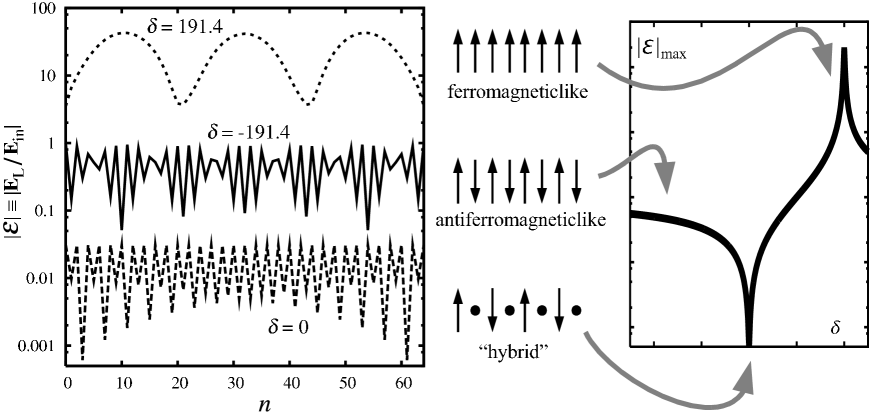
Figure 4: Strata patterns of excitation and local field in finite arrays, and their relations to the resonance tuning in the case of 64 atoms and $\delta_{\mathrm{LL}}=200$. Curves and patterns show long-wave, ferromagneticlike excitation near the Lorentz–Lorenz resonance (top curve in the left plot and top pattern in the center), counter-phase, antiferromagneticlike excitation near the anti-Lorentz edge of the band (middle curve and pattern), and hybrid excitation near the point of atomic resonance (bottom curve and pattern). Note that all the curves in the left plot show absolute normalized amplitudes of the local field. Since the fields are in general complex, their absolute amplitudes are positive, so the near-zero points in the schematic depiction of the “hybrid” mode actually correspond to the lowest points of the bottom curve in the left plot.

As we already noted, they can range from the very long ones, long-wave (LW) strata, with the maximum spatial period being double of the whole length of a 1D array, similarly to the main mode of oscillation in a violin string, to short-wave (SW) strata whereby each dipole oscillates in counter-phase to each of its nearest neighbors. The latter mode is the strongest manifestation of the fact that the array of $N$ atoms is a discrete-element resonator, akin a string of beads connected to each other, with the beads capable of the same kind of motion, when each individual bead is oscillating in counter-phase with its neighbor. Because in both cases the excitation is of dynamic nature and is due to external driving, the mechanical analogy of SW locsiton modes is more adequate than that of a static ferromagnetic configuration vs antiferromagnetic one; see also Appendix A below.

It can be immediately found, e. g. from consideration of the plots at Fig. 4, upper curve, that the LW strata emerge at the laser tuning very near to the Lorentz–Lorenz resonance, i. e. in the limit $1-\delta/\delta_{\mathrm{LL}}\ll 1$. In this case, in both FIA (20) and NNA (21), the wave number $q_{\mathrm{LW}}$ and the respective spatial wavelength $\Lambda_{\mathrm{LW}}$ are as:

$$q_{\mathrm{LW}}\approx\sqrt{1-(\delta/\delta_{\mathrm{LL}})^{2}},\qquad\Lambda_{\mathrm{LW}}=\frac{2\pi l_{a}}{q_{\mathrm{LW}}}.$$ (26)

In the infinite array, the longest $\Lambda$ is up to $2\pi l_{a}\delta_{\mathrm{LL}}$, when $\delta_{\mathrm{LL}}^{2}-\delta^{2}\sim 1$; the locsitons with longer wavelength get significantly suppressed.

The opposite limit, or the anti-Lorentz side of the locsiton band,

$$\frac{3}{4}+\frac{\delta}{\delta_{\mathrm{LL}}}\ll 1\qquad(\mbox{for NNA it is}\quad 1+\frac{\delta}{\delta_{\mathrm{LL}}}\ll 1),$$ (27)

defines SW locsitons, with

$$q_{\mathrm{SW}}\sim\pi,\qquad\Lambda_{\mathrm{SW}}/2\sim l_{a},$$ (28)

i. e. $\Lambda_{\mathrm{SW}}/2$ is the finest grain of locsiton structure, as one would expect from the “bead string” analogy. However, an incommensurability, i. e. mismatch between $\Lambda_{\mathrm{SW}}/2$ and the lattice spacing $l_{a}$, whose ratio is in general an irrational number, results in a strong spatial modulation of the SW, giving rise to a coarse LW-like structure.

In the NNA, this coarse structure of SW mode has the half-period roughly the same as for a pure LW mode, $\sim\Lambda_{\mathrm{LW}}$. This can be readily understood in terms of “beating” between the locsiton wavelength, $2\pi/q$, and the spatial scale of the discrete structure of the system, which is the normalized spacing between atoms, 1. Indeed, near the anti-Lorentz edge, $\delta+\delta_{\mathrm{LL}}\ll\delta_{\mathrm{LL}}$, we can write for a SW wavenumber: $q_{\mathrm{SW}}=\pi-\Delta q$, with $|\Delta q|\approx\sqrt{1-(\delta/\delta_{\mathrm{LL}})^{2}}=q_{\mathrm{LW}}$, and find the spatial oscillations as

$$\mathcal{E}_{n} \propto \cos(nq_{\mathrm{SW}})=\cos(n\pi-n\Delta q)$$ (29)

$$= (-1)^{n}\cos(n\Delta q),$$

with $\Delta q\approx q_{\mathrm{LW}}$, which shows alternating, counter-phase motion of the neighboring atoms, $(-1)^{n}$, modulated by a slow envelope, $\cos(nq_{\mathrm{LW}})$. Both the fine grain and the coarse modulation may be well pronounced (Fig. 4, middle curve). At $q=\pi$, the LW and SW periods converge to the same scale, $4l_{a}$, see (31) below. Using the phonon analogy, the LW locsitons may be viewed to a certain extent as counterparts to acoustic, and SW – to optical phonons.

Between those limiting points – LW locsitons at the Lorentz end of the locsiton spectrum, $\delta\sim\delta_{\mathrm{LL}}$, and SW locsitons at the anti-Lorentz end, $\delta\sim-\delta_{\mathrm{LL}}$, – there are all kinds of locsitons making chaotic looking strata (due to the above mentioned incommensurability, i. e. irrational ratio between a locsiton wavelength, $\Lambda$, and the array spacing, $l_{a}$). However, same as in the chaotic motion, there are small islands of well ordered wave patterns, located at the spectral points where the ratio $\Lambda/l_{a}$ (or $q/\pi$) is a rational number, provided that the system is at a resonance, see (35) and (36) below. One can think of them as sort of hybrids of ferromagneticlike and antiferromagneticlike behavior. Indeed, the purely antiferromagneticlike SW locsiton at $q=\pi$ is formed by the atoms with alternating polarizations,

$$\cdots\>\>\uparrow\>\>\downarrow\>\>\uparrow\>\>\downarrow\>\>\uparrow\>\>\downarrow\>\cdots\quad\mbox{for $\perp$ polarization, and}$$

$$\cdots\>\rightarrow\>\leftarrow\>\rightarrow\>\leftarrow\>\rightarrow\>\leftarrow\>\cdots\quad\mbox{for $\parallel$ polarization}.$$ (30)

This happens at $\delta\sim-\delta_{\mathrm{LL}}$ within NNA and $\delta\sim-(3/4)\delta_{\mathrm{LL}}$ for FIA. The simplest hybrid pattern is formed at $q=\pi/2$ [which is at $\delta=0$ within NNA, and $\delta/\delta_{\mathrm{LL}}=-3/32$ for a fully interacting array (20)], whereby each second atom is non-excited, while the other atoms alternate their polarization:

$$\cdots\>\uparrow\circ\downarrow\circ\uparrow\circ\downarrow\circ\uparrow\circ\downarrow\cdots\quad\mbox{for $\perp$ polarization, and}$$

$$\cdots\rightarrow\circ\leftarrow\circ\rightarrow\circ\leftarrow\circ\rightarrow\circ\leftarrow\cdots$$ (31)

$$\qquad\qquad\qquad\qquad\qquad\qquad\qquad\mbox{for $\parallel$ polarization}.$$

Examples of other simplest hybrid states within NNA are: $q=\pi/3$,  $q=\pi/4$, etc.; in general, periodic patterns exist if $q/\pi$ is a rational number, i. e. for all the eigen-resonances in finite 1D arrays within NNA, see Eq. (36) below.

Finally, it is worth noting that the strata, albeit fast-decaying, exist even beyond the locsiton band, (24). They are not, however, propagating locsitons, and their amplitudes exponentially decay with the distance. Consider the simplest case, NNA, with the losses negligibly small, $\delta^{2}>\delta_{\mathrm{LL}}^{2}\gg 1$ in (21). In this case, $\cos^{2}q>1$ in (21), which indicates that the wavenumber $q$ must be complex. Indeed, writing $q=-i\chi$ for the “Lorentz” end of the band, $\delta/\delta_{\mathrm{L}}>1$, and $q=-i\chi+\pi$ for the anti-Lorentz end, $\delta/\delta_{\mathrm{L}}<-1$ (see also Section VI below), we have the solution for $\chi$ as

$$\chi=\ln\left[|\delta/\delta_{\mathrm{LL}}|\pm\sqrt{(\delta/\delta_{\mathrm{LL}})^{2}-1}\right]$$ (32)

and for the local fields as

$$(\mathcal{E}_{n})_{\mathrm{LL}}\propto e^{\chi n}\qquad\mbox{and}\qquad(\mathcal{E}_{n})_{\mathrm{antiLL}}\propto e^{\chi n}(-1)^{n}$$ (33)

for the Lorentz and anti-Lorentz ends of the band, respectively. Here, in the case of a semi-infinite array, the sign in (32) has to be chosen such that the amplitude of the field vanishes at $|n|\to\infty$. These modes can be viewed as evanescent waves/locsitons, see also below, Section VI. One can note though that they still bear the signature of the respective locsitons on either side of the band: long-wave, almost synchronous oscillations on the Lorentz end, and short-wave, phase-alternating oscillations on the anti-Lorentz end. In general, the same patterns hold in the FIA case.

V Quantization of locsitons and field resonances in finite 1D arrays

Due to boundary conditions in (13) [or (15) within NNA], the array of $N$ atoms is a discrete-element resonator. This should result in locsiton quantization within the locsiton band (24) and corresponding size-related resonances of the local field. In a 1D array with $N$ atoms, we have $N$ coupled oscillators with the same individual atomic resonance frequency, and therefore, one should expect the original atomic line to be split into $N$ lines at most, with the collective broadened band (24) being replaced with those lines. Of course, when the dissipation (or finite linewidth of each individual line) is taken into account, those split lines will merge into one continuous locsiton band (24) if the array is sufficiently large,

$$N>\frac{7}{4}|\delta_{\mathrm{LL}}|\qquad(\mbox{or }>2|\delta_{\mathrm{LL}}|\mbox{ within NNA}).$$ (34)

The simplest result for the resonant line positions is obtained within NNA. Using the boundary condition (15), i. e. $\mathcal{E}_{0}=\mathcal{E}_{N+1}=0$, we find that the longest locsiton half-wave, corresponding to the fundamental mode, is

$$\Lambda_{1}/2=(N+1)l_{a},\qquad q_{1}=\pi/(N+1).$$ (35)

Thus, $\Lambda_{1}/2$ is the distance between nodes where LF zeros out, whereas the wavelengths $\Lambda_{k}$ of eigen-locsitons and their eigen-frequencies $\delta_{k}$, with the quantum number $1\leq k\leq N$, are respectively

$$\Lambda_{k} = \Lambda_{1}/k,\qquad\delta_{k}=\delta_{\mathrm{LL}}\cos q_{k},$$

$$q_{k} = \pi k/(N+1).$$ (36)

[Note that the first Eq. (7) in cit1 , which corresponds to the second Eq. (36) here, contained a typo (an extraneous $\pi$ in the cos argument) which we corrected here.] From these, only the resonances with odd $k$ will be realized for a symmetric driving laser profile, in particular, the uniform one, $E_{\mathrm{in}}=\mathrm{const}$ (which is the most common case here), and with even $k$ – for an anti-symmetric one, say, $E_{\mathrm{in}}=\mathrm{const}\cdot(N+1-2n)/(N-1)$, where $n$ is the sequence number of an atom in the array. In all other cases, a full set of $N$ resonances will be realized.

In essence, the size-related locsiton resonances in discrete arrays are, to a limited extent, similar to any eigen-resonances in regular continuous, i. e. non-discrete, 1D system. Examples can be found both in classical setting, e. g. a violin string, a Fabri–Perot resonator (as e. g. in a laser), and in quantum mechanics, from the resonances in a quantum well with infinitely-high walls, to electron gas in a finite layer cit11 , electrons in long molecules cit12 , etc. The major difference here is that the number of eigenmodes, or resonances, in an array with $N$ elements is limited to $N$, in contrast to the theoretically infinite number of eigenmodes in continuous finite 1D systems.

The resonances for uniform driving within NNA are shown in Fig. 2 for $\delta_{\mathrm{LL}}=200$ in the case of $N=12$ [Fig. 2(a)], $N=13$ [Fig. 2(b)], and $N=100$ [Fig. 2(c)]. One can readily find out that the lower amplitude envelope is

$$\mathcal{E}_{\mathrm{min}}(\delta)\approx 2|\bar{\mathcal{E}}|,$$ (37)

while the upper envelope of the resonant peaks within NNA for a uniform driving is

$$\mathcal{E}_{\mathrm{max}}\begin{cases}\approx|\bar{\mathcal{E}}|(n_{\delta}+n_{\delta}^{-1}),\quad\mbox{if}\quad n_{\delta}\leq 1,\\ =2|\bar{\mathcal{E}}|\quad\mbox{otherwise},\end{cases}$$ (38)

where $n_{\delta}=(N+1)/(2\sqrt{\delta_{\mathrm{LL}}^{2}-\delta^{2}})$. As $N$ increases, the resonances merge and are suppressed at $N=|\delta_{\mathrm{LL}}|O(1)$, see e. g. Fig. 2(c). However, even then $\mathcal{E}_{\mathrm{min}}$ still exceeds the uniform field $|\bar{\mathcal{E}}|$ (16) by a factor of 2. For $N=3k-1$ ($k$ is a natural number), LF amplitude dips below the lower envelope $|\mathcal{E}_{\mathrm{max}}|_{\mathrm{low}}$ at $\delta=-\delta_{\mathrm{LL}}/2$. At that frequency, within NNA, $\cos q^{\prime}=-0.5$, $q^{\prime}=2\pi/3$, and the SW period $\Lambda=3l_{a}$ is an integer of the atomic spacing, so only fine SW structure remains, resulting in an anti-resonance and in the strongest inhibition of the locsiton.

VI 1D arrays beyond the near-neighbor approximation

As we mentioned above, while the quantization of locsitons in finite arrays can be readily analyzed analytically within NNA, see the previous Sections III and V, the situation with fully-interacting arrays (FIA) presents a challenge for an analytical treatment.

Let us briefly outline general analytical and numerical results obtained so far.

• A FIA locsiton band is not symmetric with respect to the atomic resonance, $\delta=0$; it is shorter by the factor $3/4$ on the anti-Lorentz side, see (24), as opposite to the NNA.

• Respectively, FIA resonances are grouped tighter on the anti-Lorentz side of the band, albeit their number is the same as for NNA. Near the Lorentz side of the band, the NNA-predicted resonances coincide more closely with those obtained by FIA numerical calculations.

The major source of these effects is the first factor, i. e. a strongly asymmetric (with respect to the detuning frequency, $\delta$) shape of the dispersion relation, Fig. 3. A more detailed mathematical consideration of this problem, including a very good analytical fit for the dispersion relation is found in Appendix A below. Less significant, although interesting as far as the eigenmodes of 1D arrays are concerned, is the fact that simple NNA eigen-wavenumbers (36), $q_{k}=\pi k/(N+1)$, obtained based on the NNA boundary conditions $\mathcal{E}_{0}=\mathcal{E}_{N+1}=0$ [Eq. (15)] are not exact anymore. One has to use now more extended, “beyond-the-boundary” conditions (13), which are the signature of FIA, whereby

$$\mathcal{E}_{n}=0\quad\mbox{for \emph{all}}\quad n<1\quad\mbox{and}\quad n>N,$$ (39)

instead of just two end-points in NNA. To explore the problem, let us simplify it first by considering only non-dissipating atoms, $\delta_{\mathrm{LL}}^{2}\geq\delta^{2}\gg 1$, and rewrite the full-interaction dispersion relation (20) for this case as:

$$\frac{1}{S}\sum_{n=1}^{\infty}\frac{\cos(nq)}{n^{3}}=D(q)\equiv\frac{\delta}{\delta_{\mathrm{LL}}},$$ (40)

assuming $D(q)$ real. The equation for the field is written then as:

$$\mathcal{E}_{n}-\frac{1}{D}\sum_{-\infty\leq j\leq\infty}^{j\neq n}\frac{\mathcal{E}_{j}/2S}{|j-n|^{3}}=1,$$ (41)

with the boundary conditions (39).

The plot $D(q)$ for real $q$’s due to the dispersion relation (40) is shown in Fig. 3 with the solid curve. The new qualitative difference now between FIA, (40), and the NNA case, (21) without dissipation, i. e. $\cos q=D$, is as follows. With $D^{2}\leq 1$, the NNA equation has only real solutions for $q$, whereas Eq. (40), even within the locsiton band, $-3/4\leq D\leq 1$, aside from real solution for $q\equiv\tilde{q}$, has, as one can show, an infinite number of complex solutions, $q$, for each single real solution $\tilde{q}$ (i. e. for the same $D$). All of them, in addition to fast spatial oscillation terms, have a rapidly rising/falling exponential factor. These exponential modes are negligibly small almost over the entire array length, if $N\gg 1$, and they need to be accounted for only very near the end-points of the array, where they are instrumental in zeroing out the field and excitation at the points $n<1$ and $n>N$.

Let us illustrate the formation of those exponential (or evanescent) modes and their role in boundary conditions for the two-near-neighbors approximation, 2-NNA, whereby the field Eq. (41) becomes:

$$\mathcal{E}_{n}-\frac{9}{4D}\left[(\mathcal{E}_{n-1}+\mathcal{E}_{n+1})+\frac{1}{8}(\mathcal{E}_{n-2}+\mathcal{E}_{n+2})\right]=1,$$ (42)

with the boundary conditions for two pairs of end-points:

$$\mathcal{E}_{n}=0\quad\mbox{at}\quad n=0,-1\quad\mbox{and}\quad n=N+1,\,N+2.$$ (43)

The dispersion relations approximating (40) will read now as:

$$\frac{8}{9}\left[\cos q+\frac{\cos(2q)}{8}\right]=D(q),$$ (44)

see Fig. 3, long-dashed curve, and the locsiton band is determined by

$$-7/9\leq D(q)\leq 1.$$ (45)

The real solutions $\tilde{q}$ of (44) are those for which $\cos^{2}\tilde{q}\leq 1$; they give rise to strata modes of Eq. (42),

$$\mathcal{E}_{n}\propto\exp(\pm i\tilde{q}n).$$ (46)

However, having in mind that $\cos(2q)=2\cos^{2}q-1$, one can readily see that (44) has also solutions with $\cos^{2}q>1$, i. e. those that correspond to exponential modes, with complex $q=q_{\mathrm{evn2}}$. Introducing for those modes

$$q_{\mathrm{evn2}}=-i\chi+\pi$$ (47)

with real $\chi$, we obtain from (44) that for each given real $\tilde{q}$ the exponent $\chi$ is determined by:

$$\cosh\chi=4+\cos\tilde{q},$$ (48)

and the respective exponential mode is

$$(\mathcal{E}_{n})_{2}=e^{\pm(\chi+i\pi)n}=e^{\pm\chi n}(-1)^{n}.$$ (49)

Thus, these 2-NNA modes are antiferromagneticlike strata, modulated by fast exponents. Indeed, since $3\leq\cosh\chi\leq 5$, we have $1.76<\chi<2.3$.

Since the exponential, or evanescent, modes have so short “tails”, they produce relatively small correction for the respective eigen-wavelengths, $\Lambda_{n}$, and for $q_{n}$, compared to the NNA oscillatory modes, (35), (36), so that we can look for the $\Lambda_{n}$ corrected for 2-NNA at the points of resonances as:

$$\frac{\Lambda_{k}}{2l_{a}} = \frac{N+1+\Delta_{k}}{k},\qquad\Delta_{k}=O(1),$$

$$\tilde{q}_{k} = \pi\frac{2l_{a}}{\Lambda_{k}},$$ (50)

with the correction $\Delta_{k}>0$, similarly to, e. g., oscillations in a violin string with a “soft” suspension at its ends. To find $\Delta_{k}$ of the $k$-th resonance, we seek a solution for $\mathcal{E}_{n}$ as a sum of two modes: oscillatory and exponential ones. Then, for symmetric modes, i. e. with odd $k$, we have a full solution written as

$$(\mathcal{E}_{n})_{\mathrm{odd}} = \cos(\tilde{q}_{k}\bar{n})+C\cosh[\chi(\tilde{q}_{k})\bar{n}](-1)^{n},$$ (51)

$$\mbox{with}\quad\bar{n}=n-\frac{N+1}{2},$$

where $C$ is a constant. For anti-symmetric modes, with even $k$, we have:

$$(\mathcal{E}_{n})_{\mathrm{even}}=\sin(\tilde{q}_{k}\bar{n})+C\sinh[\chi(\tilde{q}_{k})\bar{n}](-1)^{n}.$$ (52)

Using now conditions (43), we can write for the points $n=-1$ and $n=0$, respectively, the following equations for the symmetric modes (51):

$$(\mathcal{E}_{-1})_{\mathrm{odd}} = \cos\left(\frac{\pi k}{2}\frac{N+3}{N+1+\Delta_{k}}\right)$$ (53)

$${}-C\cosh\left(\chi\frac{N+3}{2}\right)=0,$$

$$(\mathcal{E}_{0})_{\mathrm{odd}} = \cos\left(\frac{\pi k}{2}\frac{N+1}{N+1+\Delta_{k}}\right)$$ (54)

$${}+C\cosh\left(\chi\frac{N+1}{2}\right)=0.$$

For the anti-symmetric modes (52), one has to replace $\cos$ and $\cosh$ functions in (53), (54) with $\sin$ and $\sinh$ functions, respectively. From these two equations we can compute $\Delta_{k}$ and $C$. Indeed, approximating $\cosh(\xi)\approx\sinh(\xi)\approx e^{\xi}/2$ in (53) and (54) or in the respective equations for anti-symmetric modes, since $\chi(N+1)\gg 1$, we obtain two equations for $\Delta_{k}$ and $C$, which are readily solved for $\Delta_{k}$ and $C$ for both symmetric and anti-symmetric modes as:

$$\Delta_{k} = \frac{2}{q_{\mathrm{NNA}}}\tan^{-1}\left[\frac{\sin(q_{\mathrm{NNA}})}{e^{\chi}+\cos(q_{\mathrm{NNA}})}\right],$$ (56)

$$\mbox{with}\quad q_{\mathrm{NNA}}=\frac{\pi k}{N+1}$$

$$\mbox{and}\quad C=q_{\mathrm{NNA}}\Delta_{k}(-1)^{\bar{k}/2}e^{-\chi(N+1)},$$

where from (48), $\chi\approx\cosh^{-1}[4+\cos(q_{\mathrm{NNA}})]$, while $\bar{k}=k+1$ for symmetric modes, and $\bar{k}=k$ for the anti-symmetric ones. It is worth noting that the boundary conditions (43) at $n=N+1,N+2$ are now satisfied automatically because of our choice of the coordinate $\bar{n}$ in (51) and (52). For LW resonances, $k\ll N$, (56) reduces to

$$\Delta_{k}\approx\frac{2}{e^{\chi}+1}\approx\Delta_{\mathrm{max}}\approx\frac{2}{11},$$ (57)

which is the maximum magnitude of $\Delta_{k}$, whereas for SW resonances, $N+1-k\ll N+1$, (56) reduces to

$$\Delta_{k}\approx\frac{2}{e^{\chi}-1}\left(\frac{N+1}{k}-1\right)\approx\frac{2}{5}\left(\frac{N+1}{k}-1\right),$$ (58)

which is substantially smaller than the LW correction (57). One can readily see that $\Delta_{k}$ is a monotonically decreasing function of $k$. In the middle of the locsiton band, $k\sim(N+1)/2$, we have

$$\Delta_{k}\approx\frac{4}{\pi e^{\chi}}\approx\frac{1}{2\pi}.$$ (59)

Interestingly, a fairly good fit to (56) is provided by a much simpler formula:

$$\Delta_{k}\approx\Delta_{\mathrm{max}}\left[1-\left(\frac{k}{N+1}\right)^{3}\right].$$ (60)

Now, once the correction $\Delta_{k}$ is found, one can substitute $q=\tilde{q}_{k}=\pi k/(N+1+\Delta_{k})$, (50), into the dispersion relation (44) and calculate the respective frequency detuning for the $k$-th resonance, $D_{k}=\delta_{k}/\delta_{\mathrm{L}}$, with $k=1$ being the closest to the Lorentz–Lorenz resonance, i. e. a LW mode, and $k=N$ closest to the anti-Lorentz edge of the locsiton band, a SW mode.

A way to extend the 2-NNA approximation to a full-array interaction is to apply the result (56) for the correction of the eigen-wavenumber, $\tilde{q}_{k}$, but use it now in the full-blown dispersion relation (40), instead of the 2-NNA relation (44), to calculate the resonance detuning $\delta_{k}$. The other avenue, of course, is to seek for higher order approximations. For example, one can take into account two edge sets of 3 points each, i. e. similarly to (43), stipulate 3-NNA:

$$\mathcal{E}_{n} = 0\quad\mbox{at}\quad n=0,-1,-2$$ (61)

$$\mbox{and}\quad n=N+1,\,N+2,\,N+3.$$

Following the same route as for 2-NNA case, we obtain now, similarly to (48), a second order equation for the exponential eigenmode complex wavenumber, $q=q_{\mathrm{evn3}}$, for any given oscillation wavenumber, $\tilde{q}$, as

$$16\cos^{2}q+\cos q\,(16\cos\tilde{q}+27)$$

$$\quad{}+(104+16\cos^{2}\tilde{q}+27\cos\tilde{q})=0$$ (62)

[we leave it untransformed to $\cosh\chi$, unlike (47), (48), since in 3-NNA case the solution becomes more complicated than (49), and that transformation does not simplify the problem.] The higher-order equation for the exponential eigenmodes ensue the choice of a higher number of end-points in the boundary conditions.

It has to be noted, however, that for specifying parameters of oscillating eigenmodes, the increase of the precision by accounting for higher-order exponential modes is of very limited, if purely academic, significance. Essentially, for large arrays, $N\gg 1$, the combination of the NNA for predicting the wavenumbers $\tilde{q}$, (50) or (36), with these $\tilde{q}$’s used then in (40) to calculate the resonance eigen-frequencies $\delta$, does already a good job. A further step in increasing the precision provided by the 2-NNA corrections to eigen-wavenumbers, is to again use the corrected $\tilde{q}$’s in (40) for the same purpose, and it is more than sufficient. A special case is a small array, e. g. $N=2,3,4$, whereby it is actually preferable to simply solve the general 1D-array equations analytically, similarly to cit1 in the case of $N=2$.

VII Magic numbers

A fundamental effect of self-induced cancellation of local-field suppression emerges near the atomic resonance, $\delta=0$, at certain “magic” numbers $N$. If $\delta_{\mathrm{LL}}^{2}\gg 1$, the uniform (Lorentz–Lorenz) LF (16) at $\delta=0$ is very small, $|\bar{\mathcal{E}}|\sim|\delta_{\mathrm{LL}}|^{-1}$ [Eq. (17)]. However, in the near-neighbor approximation, if

$$N=km_{\mathrm{mag}}+1,\qquad m=1,2,3,\ldots,$$ (63)

where $m_{\mathrm{mag}}=4$ is a “magic” number within NNA, locsitons at $\delta=0$ show canceled LF suppression at some atoms. The highest cancellation is attained at $\delta=0$ and $N=5$, with the atomic dipoles lining up as in (31), whereby the LF amplitude at odd-numbered atoms is at maximum, $|\mathcal{E}_{\mathrm{max}}|\approx 1/3$, and the enhancement $|\mathcal{E}_{\mathrm{max}}/\bar{\mathcal{E}}|_{\mathrm{enh}}^{2}\approx\delta_{\mathrm{LL}}^{2}/9$ could be a few orders of magnitude; the LF at the two other atoms almost zeros out.

The self-induced cancellation effect is produced by a standing wave with the nodes at atoms with even numbers. This results in a “virtual” size-related resonance at $\delta\to 0$ (i. e. at the exact atomic resonance), which manifests itself in the enhancement (the resonant peak transpires in $|\mathcal{E}_{\mathrm{max}}/\bar{\mathcal{E}}|$ vs $\delta$). Thus, the nature of magic numbers is the coincidence of the atomic resonance with one of the size-related locsiton resonances.

The effect holds also for the interaction of each atom with all other atoms (13); the magic number in (63) takes on a “devilish” likeness here: $m_{\mathrm{mag}}=13$. It is due to the fact that for $\delta=0$ and $\delta_{\mathrm{LL}}\gg 1$, the first root $q^{\prime}$ of Eq. (20) with zero r. h. s.,

$$\sum_{n=1}^{\infty}\frac{\cos(nq^{\prime})}{n^{3}}=0,$$ (64)

has its property of $q^{\prime}/\pi$ almost coinciding with a rational number, $q^{\prime}/\pi\approx$ $6/13$  ($13q^{\prime}/6\pi=1.00026\ldots$), see Appendix A below. The locsiton wavelength is $\Lambda=2\pi/q^{\prime}=(13/3)l_{a}$, and the lowest integer of $\Lambda/2$ to exactly match an integer of $l_{a}$ is $13\,l_{a}$, which requires 14 atoms. We have now $|\mathcal{E}_{\mathrm{max}}|\approx 2/15$, with enhancement $\sim 4\delta_{\mathrm{LL}}^{2}/225$.

As we have shown in cit1 , 2D lattices can also exhibit “magic shapes” with similar properties; the simplest one within NNA is a six-point star with an atom at its center, thus making the total number of atoms again $N=13$. More details on magic shapes for 2D lattices will be discussed by us elsewhere.

VIII Traveling locsiton waves: velocity and penetration depth

If the locsitons are waves, can they be excited outside the driving field area? and thus travel away from the Lorentz–Lorenz uniform local field area? how far can they travel before being extinguished? how fast do they propagate? having in mind their dissipation, what is the size of a finite array to have well pronounced standing waves and size-related resonances?

Of course, the locsitons can propagate in an array even in the areas unaccessible for the external (laser) field. If the spatial profile gradient of the driving wave is large enough, a LF excitation can be found beyond the driving field area; the terminological irony here is that the local-field phenomenon is due to a nonlocal interaction, and the locsitons can propagate away from their origination point. This may happen when the external laser field is non-uniform and has a large gradient, e. g. when one entirely screens out a part of the array by imposing a “sharp knife” over the array.

Even simpler and more transparent case is when only an end-point of a semi-infinite 1D array [say, with $n=1$ in (13)] is illuminated by a laser field via a pin-hole. Eq. (13) has then non-zero (unity) r. h. p. for $n=1$ only, and the r. h. p. zeroes out at all the other points. In this case, no Lorentz–Lorenz local field exists for any atom at $n>1$, and the only field and atomic excitation passed along the array of atoms will be locsitons. This may be the best way to excite and observe “pure” locsitons, with them not being masked by any external, averaged, mean, etc., fields. With such an arrangement, the 1D array (or a sufficiently thin atomic “cylinder” or carbon nanotube) becomes a true and effective waveguide for locsitons, capable of transmitting non-diffracting radiation and atomic excitation from one location (e. g. in opto-electronic circuits) to another.

The main issue here is how far the locsiton can propagate. One can investigate it by studying the dispersion relation (20) or (21), which predicts not only the locsiton wavenumbers, $q^{\prime}\equiv\mathrm{Re}(q)$, for any given frequency detuning $\delta$, but also their dissipation depth or distance (in terms of numbers of atoms) for each wavenumber, as $N_{\mathrm{dis}}=1/q^{\prime\prime}$ where $q^{\prime\prime}\equiv\mathrm{Im}(q)$. Using only the NNA dispersion relation (21), amply sufficient here, since the calculation of the dissipation distance doesn’t require the same precision as for the real wavenumbers, we find out that the exact solutions for $q^{\prime}$ and $q^{\prime\prime}$ are determined by:

$$\cos^{2}(q^{\prime}) = \frac{1}{2}\left(1+\frac{\delta^{2}+1}{\delta_{\mathrm{LL}}^{2}}\right)$$ (65)

$${}-\sqrt{\frac{1}{4}\left(1+\frac{\delta^{2}+1}{\delta_{\mathrm{LL}}^{2}}\right)^{2}-\frac{1}{\delta_{LL}^{2}}}$$

and

$$\sinh^{2}(q^{\prime\prime}) = -\frac{1}{2}\left(1-\frac{\delta^{2}+1}{\delta_{\mathrm{LL}}^{2}}\right)$$ (66)

$${}+\sqrt{\frac{1}{4}\left(1-\frac{\delta^{2}+1}{\delta_{\mathrm{LL}}^{2}}\right)^{2}+\frac{1}{\delta_{\mathrm{LL}}^{2}}}.$$

From (65), for very small dissipation, i. e. when $\delta_{\mathrm{LL}}^{2}>\delta^{2}\gg 1$, we have, as expected,

$$\cos(q^{\prime})\approx\frac{\delta}{\delta_{\mathrm{LL}}}.$$ (67)

The dissipation length in terms of the numbers of atoms, $N_{\mathrm{dis}}=1/q^{\prime\prime}$, is readily found from (66). At the exact atomic resonance, $\delta=0$, if $\delta_{\mathrm{LL}}^{2}\gg 1$, we have:

$$q^{\prime\prime}\approx\frac{1}{|\delta_{\mathrm{LL}}|},\qquad N_{\mathrm{dis}}\approx|\delta_{\mathrm{LL}}|.$$ (68)

In general, in the most part of the locsiton band (except for the edge areas, $\delta_{\mathrm{LL}}^{2}-\delta^{2}\lesssim 1$), we find that

$$q^{\prime\prime}\approx\frac{1}{\sqrt{\delta_{\mathrm{LL}}^{2}-\delta^{2}}},\qquad N_{\mathrm{dis}}\approx\sqrt{\delta_{\mathrm{LL}}^{2}-\delta^{2}}.$$ (69)

Finally, at the locsiton band edges, defined as $\delta_{\mathrm{LL}}^{2}-\delta^{2}=1$, (66) results in

$$q^{\prime\prime}\approx\frac{1}{\sqrt{\delta_{\mathrm{LL}}}},\qquad N_{\mathrm{dis}}\approx\sqrt{\delta_{\mathrm{LL}}},$$ (70)

and it remains roughly the same as $\delta^{2}$ reaches $\delta_{\mathrm{LL}}^{2}$.

Thus, in the most of the locsiton band, the dissipation length, in terms of the numbers of atoms, is $N_{\mathrm{dis}}=O(\delta_{\mathrm{LL}})$, which also determines the maximum size of array to still enable the size-related resonances, in agreement with Section V.

Let us address now the characteristic velocities of the locsitons. Neglecting decay in (21) ($\delta_{\mathrm{LL}}^{2}>\delta^{2}\gg 1$), the group velocity of locsitons, $v_{\mathrm{gr}}=l_{a}(d\omega/dq)$, is found as:

$$v_{\mathrm{gr}}=\frac{l_{a}}{T}\frac{d\delta}{dq},\qquad\cos q=\frac{\delta}{\delta_{\mathrm{LL}}},$$ (71)

hence

$$\frac{dq}{d\delta} = -\frac{1}{\sqrt{\delta_{\mathrm{LL}}^{2}-\delta^{2}}},$$

$$v_{\mathrm{gr}} = l_{a}\sqrt{\Omega_{\mathrm{R}}^{2}-\Delta\omega^{2}}=v_{\mathrm{R}}\sqrt{\delta_{\mathrm{LL}}^{2}-\delta^{2}},$$ (72)

where $\Omega_{\mathrm{R}}$ is the Rabi frequency of the self-interacting array (25), and $v_{\mathrm{R}}=\Omega_{\mathrm{R}}l_{a}$ is a characteristic Rabi speed,

$$\frac{v_{\mathrm{R}}}{c}=\alpha\left|\frac{d_{a}}{el_{a}}\right|^{2}O(1)\ll 1,$$ (73)

which could be even slower than a typical speed of sound in condensed matter. This effect can be used e. g. for developing nano-size delay lines in molecular computers and in optical gyroscopes. The LW-locsiton phase velocity is

$$v_{\mathrm{ph}}\approx\frac{v_{\mathrm{R}}^{2}}{v_{\mathrm{gr}}}.$$ (74)

IX Nonlinear excitation of a 1D array; optical bistability and hysteresis

So far we studied linear (in field) excitations of atomic 1D arrays. The nonlinear interactions open door to a huge new landscape of effects. The simplest and very generic nonlinearity in a two-level system is the saturation of its absorption (4), (5), which translates into a nonlinear response of the atom polarization to the local field (6); this, in turn, nonlinearly affects the strength of interaction between atoms (9). This represents a rare case whereby the nonlinear change (decrease) of absorption directly affects the eigen-frequencies of the system (1D array), by directly reducing the interaction. Many nonlinear effects are brought up in short pulse modes, e. g. discrete solitons, to be considered by us elsewhere. However, spectacular effects, such as hysteresis and optical bistability, emerge even in cw mode.

To write a set of nonlinear equations for an infinite 1D array, we first scale all fields to the characteristic saturation field, $E_{\mathrm{sat}}$ (5), instead of scaling to the incident field, $E_{\mathrm{in}}$, so that the dimensionless local fields at the $n$-th atom, $Y_{n}$, and the incident field, $X$, are

$$X=E_{\mathrm{in}}/E_{\mathrm{sat}},\qquad Y_{n}=E_{n}/E_{\mathrm{sat}},$$ (75)

and the nonlinear counterpart of (13) and (14) for the array is written now as:

$$Y_{n}-\delta_{\mathrm{LL}}(\delta-i)\sum_{\mathrm{latt}}^{j\neq n}\frac{Y_{j}/2S}{|j-n|^{3}(1+\delta^{2}+|Y_{j}|^{2})}=X,$$ (76)

where $\delta_{\mathrm{LL}}$ is defined by (16), so it covers either incident polarization. The nonlinear counterpart of the NNA equation (15) is now

$$Y_{n}-\frac{\delta_{\mathrm{LL}}(\delta-i)}{2}\left(\frac{Y_{n-1}}{1+\delta^{2}+|Y_{n-1}|^{2}}\right.$$

$$\qquad\qquad\left.{}+\frac{Y_{n+1}}{1+\delta^{2}+|Y_{n+1}|^{2}}\right)=X,$$ (77)

$$\mathcal{E}_{0}=\mathcal{E}_{N+1}=0.$$

None of this is an easy object even for numerical solution, let alone analytical one. We have, however, derived in cit1 a closed analytical solution for the nonlinear mode in the most fundamental system – an array of just two atoms – and found bistability and hysteresises in such a mode. In this paper, more as a matter of illustration, we find an analytical multistable solution and hysteresis for the simplest case of Lorentz–Lorenz uniform field; however, our computer simulations showed that multistability and hysteresises exist in the vicinity of each size-related resonance in the system.

For the sake of simplicity, we consider here the case of Lorentz–Lorenz uniform mode. In the near-neighbor approximation (77) [the FIA results will essentially differ only by a factor of $O(1)$], we have $Y_{n}=Y_{n-1}=Y_{n+1}\equiv Y$, and thus the nonlinear equation for the uniform local field, $Y$, is

$$Y\left[1-\frac{\delta_{\mathrm{LL}}(\delta-i)}{1+\delta^{2}+|Y|^{2}}\right]=X,$$ (78)

or for the field intensity, $|Y|^{2}\equiv y$,

$$y\,\frac{[1-\delta(\delta_{\mathrm{LL}}-\delta)+y]^{2}+\delta_{\mathrm{LL}}^{2}}{(1+\delta^{2}+y)^{2}}=X^{2}.$$ (79)

It can be readily seen that the strongest nonlinear effect emerges near the Lorentz–Lorenz resonance, $\delta\approx\delta_{\mathrm{LL}}$. Assuming small losses, $\delta,\delta_{\mathrm{LL}}\gg 1$, we can analyze the threshold of the multistability and hysteresis mode by stipulating that $y\ll\delta_{\mathrm{LL}}^{2}$,  $\Delta\equiv\delta_{\mathrm{LL}}-\delta\ll\delta_{\mathrm{LL}}$, and thus (79) can be further simplified as

$$y[(y-\delta_{\mathrm{LL}}\Delta)^{2}+\delta_{\mathrm{LL}}^{2}]/\delta_{\mathrm{LL}}^{4}\approx X^{2}.$$ (80)

The threshold for the multistable solution $y(X)$ of this equation is determined by the condition $dX/dy=d^{2}X/dy^{2}=0$, which results in the critical requirement that

$$\Delta\equiv\delta_{\mathrm{LL}}-\delta > \Delta_{\mathrm{cr}}=\sqrt{3},$$

$$y\equiv|Y|^{2} > y_{\mathrm{cr}}=\frac{2}{\sqrt{3}}\delta_{\mathrm{LL}},$$ (81)

$$X^{2} > X_{\mathrm{cr}}^{2}=\frac{1}{\delta_{\mathrm{LL}}^{2}}\left(\frac{2}{\sqrt{3}}\right)^{3}.$$

Amazingly, as one recalls that $X=E_{\mathrm{in}}/E_{\mathrm{sat}}$ and $\delta_{\mathrm{LL}}\gg 1$, the critical (threshold) driving intensity $E_{\mathrm{in}}^{2}$ to initiate multistability and hysteresis could be orders of magnitude lower than the saturation one, $E_{\mathrm{sat}}^{2}$, which is mostly due to resonant nature of the effect that emerge in the vicinity of the Lorentz–Lorenz resonance. Thus, the required saturation nonlinearity is indeed just a slight perturbation to the resonant linear mode. This should be of no big surprise, since the nature of the effect is the same as in many other so called vibrational hysteresises cit13 in resonant nonlinear systems, from pendulum cit13 to electronic circuits cit14 , to optical bistability in a Fabri–Perot resonator cit15 , to a cyclotron resonance of a slightly relativistic electron cit16 . In all these nonlinear resonances, it is enough for a narrow resonant curve to be tilted beyond its resonance width to reach multistability by becoming a “Pisa-like tower”.

The formation of bistability and hysteresis is depicted in Fig. 5, where the resonant curve $Y(\delta)$ is shown for different driving $X$ for the full equation (79).

Figure 5: Multistability of Lorentz–Lorenz mode in a long array: local Lorentz field amplitude $Y$ vs detuning $\delta$ for different normalized driving amplitudes $X=E_{\mathrm{in}}/E_{\mathrm{sat}}$ for the case of $\delta_{\mathrm{LL}}=100$.

The formation of a tri-stable solution results in the so called bistability, whereby only the states with the maximum and minimum intensities are stable, whereas the middle branch of the solution is absolutely unstable. To an extent, it is similar to one of the hysteretic patterns for the local field found for the case of the local field cit1 and scattered light cit17new of just two atoms; the hysteretic resonance here is produced by a Lorentz-like, or ferromagneticlike, excitation of atoms with LW locsitons. This effect is also reminiscent of optical intrinsic bistability for uniform LF in dense materials predicted earlier in cit17 and observed experimentally in cit18 .

The above result for hysteresis and bistability was found for the uniform, Lorentz, field, i. e. near the Lorentz–Lorenz resonance, using a simple field distribution. However, it is clear from the above argument with a “Pisa-like tower”, a similar hysteretic effect can be expected in the close vicinity of every size-related locsiton resonance within the locsiton band. Some of the most interesting hysteresises, though, are excited for the SW locsitons, when the nearest atoms counter-oscillate in an antiferromagneticlike fashion, as shown in cit1 for the anti-Lorentz band edge for two atoms. This hysteresis results in a “split-fork” bistability and will be discussed by us in application to long arrays elsewhere.

X Analogies to locsitons in other physical systems and general discussion

It is only natural to expect the effects studied here to manifest themselves in other finite systems of discrete resonant oscillators that are externally driven and interact with each other. On the one hand, this may help to demonstrate and verify some major results reported here in much simpler and easily handleable settings; on the other hand, this may bring up new features in these other systems that escaped attention in seemingly well developed and researched fields. We consider here a few such systems.

Perhaps, the most classical example would be a mechanical finite array of identical physical pendulums with the same individual resonant frequencies, weakly coupled to each other (say, by using weak strings between neighboring pendulums), with each pendulum driven independently by an external feed (say, via EM solenoids) with the same phase for all of them. By tuning the frequency of the driving feed around the resonant frequency of the pendulums, one may expect to observe stratified excitation of the pendulums, from long-wave, ferromagneticlike strata, to short-wave, antiferromagneticlike ones. One can also expect to observe “magic” numbers and related effect of non-moving pendulums surrounded by strongly excited ones. (It is worth noting that we are talking here about a cw motion, in contrast to the well known effect in two coupled non-driven pendulums, whereby the pendulums periodically alternate periods of zero-excitation in one and strong excitation in the other one, with the frequency of the alternation being inversely proportional to the coupling.) The major effect here would be again due to locsitons, and the major critical condition for their excitation would be similar to the condition on the strength of interaction, $Q_{a}$, (10), to exceed a critical one.

The driven pendulum array would be a great classroom-demonstration tool. However, although purely mechanical, it might take some effort to implement, due to the need of an independent feed to each pendulum. From that point of view, a much simpler, easily implementable, controllable, recordable, and versatile system could be an electronic array of individual resonant circuits, electronically coupled to each other. A long while ago, similar systems have been used as transmission lines, whereas a finite set of circuits has also been of interest for such applications as bandpass filters. However, the detailed picture of behavior of individual circuits inside such systems have apparently not attracted too much attention, with a few reasons for that. The main difference between these systems and the ones proposed by us, is that we need an independent feed with the same phase for each individual circuit, which may be arranged, by e. g. using individual cable for each one of them. The coupling between the individual circuits can be engineered in such a way that one can arrange strictly near-neighbor interaction, two-near-neighbors interaction, etc. Besides, the contribution of each neighboring circuit can be independently controlled, so the term $1/n^{3}$ can now be changed to any desirable function of the neighbor spacing.

A close example, which might have important implications for large radio-frequency antenna arrays, for e. g. radio-astronomy applications, as well as in multi-dish radar systems, is the interaction of radiators in those arrays, if the strength of this interaction exceeds some critical value.

Since in the case of electronic circuits the polarization of the feed and the spatial anisotropy as in (2) is not a factor anymore, the dipole-like interaction is simplified, as its spatial polarization form-factor $F_{(p)}$ (as in Section III) can be now dropped, and the equations of motion (13)–(16) can be simplified. Furthermore, since now the direction of a “dipole” with respect to the “incident polarization” is not a factor, one can arrange a loop or ring of those circuits, instead of a linear 1D array, which allows for periodic boundary condition instead of zero boundary conditions as e. g. in (13). This would greatly simplify the theory and comparison with the experiment, on the one hand, and allow for new interesting effects in ring arrays (such as e. g. greatly enhanced Sagnac effect and related gyroscope applications), to be discussed by us elsewhere, on the other hand.

An interesting and exotic opportunity with 1D arrays, and especially ring arrays, is a possibility to develop a toy model of “discrete space quantum mechanics”, whereby a wave function is replaced by a set of oscillating fields at discrete spatial points, instead of a regular wave distributed in space. This discrete-space quantum mechanics (QM) could be of interest for the theory of certain systems, as well as from fundamental point of view; for example, the ring arrays then would allow to build a theory of a Bohr-like “discrete-QM H atom”, with finite number of primary quantum numbers, unlike an infinite numbers of quantum levels as in a regular-QM H atom.

A very interesting analogy, especially from the application point of view, is magnetic spin resonance, in particular nuclear magnetic resonance (NMR) cit19 , as well as magnetic resonances in finite spin systems, in particular so called molecular magnets cit20 . They have some common points with the interacting systems considered here, in particular, two-level nature of resonances in both systems.

In optical domain, an observation of the effect discussed here can be done in a few ways. Nanostrata and locsitons can be observed either via size-related resonances in scattering of laser radiation, or via X-ray or electron energy loss spectroscopy of the strata.

The effect has promising potential for molecular computers cit21 and nanodevices. The major advantage of locsitons vs electrons in semiconductors is that they are not based on electric current or charge transfer. This may allow for a drastic reduction of the size limit for computer logic elements currently based on metal-oxide-semiconductor technology, which may suffer from many irreparable problems on a scale below 10 nm. As such, locsiton-based devices could be an interesting entry into the field, as complimentary or alternative to emerging technologies like plasmonics cit22 or spintronics cit23 . They can offer both passive (e. g. transmission lines and delays), and active elements, e. g. for switching and logics. A ring-array may be used as a basis for a Sagnac-locsiton-based gyroscope; low locsiton velocity may allow for a high sensitivity in a small ring.

Another promising application of locsitons could be biosensing devices, where target-specific receptor molecules either form a locsiton-supporting lattice or are attached to its sites; a localized locsiton occurs whenever a target biomolecule attaches to a receptor.

Finally, exciting opportunities exist in atomic arrays and lattices with inverse population created by an appropriate (e. g. optical) pumping, which may lead to a laser-like locsiton stimulated emitter (“locster”), to be discussed elsewhere.

XI Conclusions

In conclusion, in this study of strong stratification of local field and dipole polarization in finite groups of atoms predicated by us earlier cit1 , we developed a detailed theory of the phenomenon in one-dimensional arrays of atom or resonant particles. In strong departure from Lorentz–Lorenz theory, the spatial period of those strata may become much shorter than the incident wavelength. By exploring nanoscale elementary excitations, locsitons, and resulting size-related resonances and large field enhancement in finite arrays of atoms, we showed that their spatial spectrum has both long waves, reminiscent of ferromagnetic domains, and super-short waves corresponding to the counter-oscillating neighboring polarizations, reminiscent of antiferromagnetic spins. The system also exhibits “hybrid” modes of excitation that have no counterpart in magnetic ordering, and are more representative of the effect. Our theory that goes beyond Ising-like near-neighbor approximation and describes the excitation whereby each atom interacts with all the other atoms in the array, reveals the existence of infinite spectrum of “exponential”, or “evanescent” eigenmodes in the such arrays. We explored the phenomenon of “magic” numbers of atoms in an array, whereby resonant local-field suppression can be canceled for certain atoms in an array. We also demonstrated the existence of nonlinearly induced optical bistability and hysteresis in the system. We discussed a stratification effect similar to that in atomic arrays, which may exist in broad variety of self-interacting systems, from mechanical (pendulums) to electronic circuits, to radar arrays, and to the nuclear magnetic resonance. We pointed out a few potential applications of the atomic and similar arrays in such diverse field as low-losses nano-elements for optical computers, small-size Sagnac-effect-based gyroscopes, and bio-censors.

XII Acknowledgements

The authors appreciate helpful discussions with V. Atsarkin and R. W. Boyd. This work is supported by AFOSR.

Appendix A Mathematical aspects of the dispersion equation (20)

In this Appendix we consider mathematical properties of the Fourier series in the dispersion relation (20), i. e. the function

$$\Sigma_{\rho}(q)\equiv\sum_{n=1}^{\infty}\frac{\cos(nq)}{n^{\rho}},$$ (82)

which is a generalized form of (20) [in (20), $\rho=3$ due to the chosen geometry of the problem – 1D array of point dipoles], but we will restrict ourselves to natural numbers $\rho$. Note, for example, that in the case of infinite “dipole strings”, parallel to each other and equidistantly arranged in a 2D plane, $\rho=2$, whereas for “dipole planes” parallel to each other and equidistantly arranged in the 3D space, $\rho=1$.

Our main purpose here is to find a closed finite analytical form of the function $\Sigma_{\rho}(q)$ that originated the Fourier series (82), and when it is impossible in terms of more or less regular analytical functions, at least find a closed finite derivative $d^{m}\Sigma_{\rho}(q)/dq^{m}$ with minimum derivative order $m$, which will help us to analyze in great detail the behavior of the function $\Sigma_{\rho}(q)$ in its physically interesting points, e. g. at $q=0,\pi$, the ratio of its min/max values $\Sigma_{\rho}(\pi)/\Sigma_{\rho}(0)$, etc. Those derivatives are actually the main tool in our search. Indeed, differentiating $\Sigma_{\rho}(q)$ in (82) $\rho-1$ times, one obtains

$$\frac{d^{\rho-1}\Sigma_{\rho}(q)}{dq^{\rho-1}} = (-1)^{\rho/2}\sum_{n=1}^{\infty}\frac{\sin(nq)}{n},$$

$$\qquad\qquad\mbox{if}\quad\rho=2,4,6,\ldots$$

and

$$\frac{d^{\rho-1}\Sigma_{\rho}(q)}{dq^{\rho-1}} = (-1)^{(\rho-1)/2}\sum_{n=1}^{\infty}\frac{\cos(nq)}{n}$$

$$= (-1)^{(\rho-1)/2}\Sigma_{1}(k),\qquad\mbox{if}\quad\rho=1,3,5,\ldots$$

Recalling that $\sin\xi=(e^{i\xi}-\mathrm{c.c.})/2i$ and $\cos\xi=(e^{i\xi}+\mathrm{c.c.})/2$, we recognize the sums $\sum_{n=1}^{\infty}e^{\pm inq}/n$ in (A) and (A) as Taylor expansions of $-\ln(1-e^{\pm iq})$.

In the case of even numbers $\rho$, the sum (A) in the interval $0,2\pi$ (which is of the most interest) yields:

$$\sum_{n=1}^{\infty}\frac{\sin(nq)}{n}=\begin{cases}\displaystyle\frac{\pi\mathop{\mathrm{sign}}(q)-q}{2},&\quad\mbox{if}\quad|q|\in(0,2\pi),\\ 0,&\quad\mbox{if}\quad|q|=0,2\pi.\end{cases}$$ (85)

It is discontinuous at $q=0,\pm 2\pi$. Even numbers $\rho$ are thus a “lucky” case; the result (85) is easily integrated to restore function $\Sigma_{\rho}(q)$. In a physically interesting case, $\rho=2$, by integrating (85) once we have

$$\Sigma_{2}(q) \equiv \sum_{n=1}^{\infty}\frac{\cos(nq)}{n^{2}}=\frac{3(\pi-|q|)^{2}-\pi^{2}}{12},$$

$$\qquad\qquad\mbox{if}\quad q\in[-2\pi,2\pi],$$

which is a continuous (but not smooth) function with $\Sigma_{2}(0)=\pi^{2}/6$ and $\Sigma_{2}(\pi)=-\pi^{2}/12$, so that $(\Sigma_{2})_{\mathrm{min}}/(\Sigma_{2})_{\mathrm{max}}=-1/2$.

As to the closed integrability, one is not as lucky with odd numbers $\rho$; the summation of (A) yields:

$$\Sigma_{1}(q)\equiv\sum_{n=1}^{\infty}\frac{\cos(nq)}{n}=-\ln[2\,|\sin(q/2)|],$$ (87)

$$\quad\mbox{i.\,e.}\quad\Sigma_{1}(q)\to\infty\quad\mbox{at}\quad q=2m\pi,$$

which cannot be integrated in simple known analytical functions, but it gives a good analytical tool to analyze the behavior of $\Sigma_{\rho}(q)$. In the case of most interest to us, $\rho=3$, we have that near the maximum of $\Sigma_{3}$ at small wavenumbers

$$\Sigma_{3}(q)\approx S+\frac{q^{2}}{2}\left(\ln|q|-\frac{3}{2}\right)\qquad\mbox{at}\quad|q|\ll 1,$$ (88)

where $S=\sum_{j=1}^{\infty}j^{-3}\approx 1.202057$, whereas near the minimum of $\Sigma_{3}$, i. e. near $q=\pi$, we have

$$\Sigma_{3}(q)\approx-\frac{3S}{4}+\frac{(q-\pi)^{2}}{2}\ln 2,\qquad\mbox{if}\quad|q-\pi|\ll 1.$$ (89)

Notice that here $(\Sigma_{3})_{\mathrm{min}}/(\Sigma_{3})_{\mathrm{max}}=-3/4$, and $d^{2}\Sigma_{3}/dq^{2}=0$ at $q=2m\pi\pm\pi/3$.

For the magic numbers in the case of full interaction of individual atoms with all the other atoms in the array, it is important to know zeros of the function $\Sigma_{3}(q)$. As it has been mentioned before [see (64) and related text], it turns out that the value of the ratio $q^{\prime}/\pi$ for the first positive root of the equation $\Sigma_{3}(q)=0$ is very close to a small rational number:

$$\frac{q^{\prime}}{\pi}=(1+\Delta^{\prime})\cdot\frac{6}{13},\qquad\mbox{with}\quad\Delta^{\prime}\approx 2.6\times 10^{-4}.$$ (90)

For all practical purposes, a good approximation for $\Sigma_{3}(q)$ is provided by:

$$\Sigma_{3}^{\mathrm{(fit)}}(q)=S\left\{\cos q\phantom{\frac{1}{1}}\right.$$

$$\quad\left.{}+\frac{\ln[(S+\Delta S)|\sin(q/2)|]}{\ln(S+\Delta S)}\cdot\frac{\sin^{2}(q/2)}{4}\right\},$$ (91)

where $\Delta S=0.01472$. It coincides with the results provided by numerical summation of (82) with $\rho=3$ with the precision better than $0.6\%$ of $S$, and their zeros coincide with each other and with (90) with precision better than $10^{-6}$.

Let us also prove the relation for $(\Sigma_{\rho})_{\mathrm{min}}/(\Sigma_{\rho})_{\mathrm{max}}$ used in (23). Indeed,

$$\frac{D(\pi,\rho)}{D(0,\rho)}=\frac{(\Sigma_{\rho})_{\mathrm{min}}}{(\Sigma_{\rho})_{\mathrm{max}}}=\frac{\displaystyle\sum_{n=1}^{\infty}(-1)^{n}n^{-\rho}}{\displaystyle\sum_{n=1}^{\infty}n^{-\rho}}$$

$${}=\frac{\displaystyle-\sum_{n=1}^{\infty}n^{-\rho}+2\sum_{m=1}^{\infty}(2m)^{-\rho}}{\displaystyle\sum_{n=1}^{\infty}n^{-\rho}}$$ (92)

$${}=\frac{\displaystyle-\sum_{n=1}^{\infty}n^{-\rho}+2^{-\rho+1}\sum_{n=1}^{\infty}n^{-\rho}}{\displaystyle\sum_{n=1}^{\infty}n^{-\rho}}=-1+\frac{1}{2^{\rho-1}}.$$

Note that (92) is valid for any number $\rho>1$.

References

- (1) A. E. Kaplan and S. N. Volkov, Phys. Rev. Lett. 101, 133902 (2008).
- (2) M. Born and E. Wolf, Principles of Optics, (Cambridge Univ. Press, Cambridge, 1997), Sections 2.3 and 2.4; J. Van Kranendonk and J. E. Sipe, in Progress in Optics, vol. 15, ed. E. Wolf, (N. Holland, Amsterdam, 1977), p. 245.
- (3) A. Aharoni, Introduction to the Theory of Ferromagnetism (Oxford Univ. Press, Oxford, 2001).
- (4) L. D. Landau and E. M. Lifshitz, The Classical Theory of Fields (Butterworth, New York, 1980).
- (5) A. Yariv, Quantum Electronics, (Wiley, New York, 1989); V. S. Butylkin, A. E. Kaplan, Yu. G. Khronopulo, and E. I. Yakubovich, Resonant nonlinear interactions of light with matter, (Springer-Verlag, New York, 1989); V. S. Butylkin, A. E. Kaplan, and Yu. G. Khronopulo, Sov. Phys. JETP 32, 501 (1971); C. M. Bowden and J. P. Dowling, Phys. Rev. A 47, 1247 (1993).
- (6) J. J. Maki, M. S. Malcuit, J. E. Sipe, and R. W. Boyd, Phys. Rev. Lett. 67, 972 (1991).
- (7) D. G. Steel and S. C. Rand, Phys. Rev. Lett. 55, 2285 (1985).
- (8) C. Kittel, Introduction to Solid State Physics (Wiley, New York, 1996).
- (9) E. Yablonovitch, Phys. Rev. Lett. 58, 2059 (1987).
- (10) V. B. Sandomirskii, Sov. Phys. JETP 25, 101 (1967); M. C. Tringides, M. Jałochowski, and E. Bauer, Phys. Today, 60, No. 4, 50 (2007).
- (11) V. Chernyak, S. N. Volkov, and S. Mukamel, Phys. Rev. Lett. 86, 995 (2001).
- (12) J. J. Stoker, Nonlinear vibrations in mechanical and electrical systems (Interscience, New York, 1950).
- (13) A. E. Kaplan, Radio Eng. Electron. Phys. 8, 1340 (1963); A. E. Kaplan, Yu. A. Kravtsov, and V. A. Rylov, Parametric oscillators and frequency dividers (Sov. Radio, Moscow, 1966), in Russian.
- (14) H. M. Gibbs, S. L. McCall, and T. N. C. Venkatesan, Phys. Rev. Lett. 36, 1135 (1976); H. M. Gibbs, Optical Bistability, (Academic Press, New York, 1985).
- (15) A. E. Kaplan, Phys. Rev. Lett. 48, 138 (1982); ibid. 56, 456 (1986).
- (16) O. N. Gadomskii and Yu. Yu. Voronov, J. Appl. Spectr. 67, 517 (2000); O. N. Gadomskii and Yu. Abramov, Opt. Spectr. 93, 879 (2002).
- (17) C. M. Bowden and C. C. Sung, Phys. Rev. A 19, 2392 (1979).
- (18) M. P. Hehlen, H. U. Güdel, Q. Shu, J. Rai, S. Rai, and S. C. Rand, Phys. Rev. Lett. 73, 1103 (1994).
- (19) S. I. Doronin, E. B. Fel’dman, and S. Lacelle, Chem. Phys. Lett. 353, 226 (2002).
- (20) J. R. Long, in Chemistry of Nanostructured Materials, ed. P. Yang (World Scientific, Hong Kong, 2003).
- (21) J. R. Heath and M. A. Ratner, Phys. Today, 56, No. 5, 43 (2003).
- (22) A. K. Sarychev and V. M. Shalaev, Electrodynamics of Metamaterials, (World Scientific, Hong Kong, 2008); W. A. Murray and W. L. Barnes, Adv. Mater. 19, 3771 (2007); Surface Plasmon Nanophotonics, eds. M. L. Brongersma and P. G. Kik (Springer, New York, 2007); Y. Fainman, K. Tetz, R. Rokitski, and L. Pang, Opt. Photonics News, 17, No. 7, 24 (2006).
- (23) I. Žutić, J. Fabian, and S. Das Sarma, Rev. Mod. Phys. 76, 323 (2004).