XIM: A virtual X-ray observatory for hydrodynamic simulations

Abstract

We present a description of the public code XIM , a virtual X-ray observatory. XIM can be used to convert hydrodynamic simulations of astrophysical objects, such as large scale structure, galaxy clusters, groups, galaxies, supernova remnants, and similar extended objects, into virtual X-ray observations for direct comparison with observations and for post-processing with standard X-ray analysis tools. By default, XIM simulates Chandra and the International X-ray Observatory IXO , but can accommodate any user-specified telescope parameters and instrument responses. Examples of XIM applications include virtual Chandra imaging of simulated X-ray cavities from AGN feedback in galaxy clusters, kinematic mapping of cluster velocity fields (e.g., due to mergers or AGN feedback), as well as detailed spectral modeling of multi-phase, multi-temperature spectra from space plasmas.

1. Introduction

As the peaks of the matter distribution in the cosmic web of structure formation, clusters hold a special place in cosmology. The ever-increasing power of computers has made direct hydrodynamic simulation of complex astrophysical systems a reality. We can now simulate large cosmological boxes that include massive clusters of galaxies and incorporate complex physical phenomena (such as star formation, the energy input from black holes, metallicity injection from supernovae, to name a few).

X-ray observations of clusters have proven to be a rich and powerful tool to study large scale structure. The launch of the Chandra X-ray Observatory in particular has revealed a wealth of new information on cluster dynamics and at the same time, posed a number of new puzzles, such as the question of how clusters maintain their core temperature against catastrophic cooling.

While hydro simulations can address many of these questions, it is vital that the output data from such simulations can be compared with X-ray observations in the most direct and faithful way possible. Generally, galaxy cluster are simple to simulate compared to, for example, galaxies, where complex ISM physics and star formation seriously complicate modeling. For that reason, it is much easier to produce realistic simulations of clusters that can be faithfully compared with observations.

This comparison requires computer codes that can turn the output from a hydro simulation into a virtual observation with a given X-ray telescope — a virtual X-ray observatory.

In this paper, we present such a virtual telescope, the IDL code XIM , which is now publically available at the web site
http://www.astro.wisc.edu/$\sim$heinzs/XIM

XIM is best suited to process output from Eulerian (grid–based) hydro codes and its direct application is the virtual observation of thermal emission from cosmic gas. While it was written to directly simulate Chandra and the next generation X-ray observatory IXO , it can be adapted to simulate any arbitrary X-ray telescope for a set of user-supplied response matrix files.

Since X-ray telescopes are imaging spectrographs (each photon is time– and energy–tagged, thus allowing a time– and energy–resolved image to be constructed), the output from a virtual X-ray observation is a spectral imaging cube (such as would be obtained from an integral field spectrograph in optical spectroscopy, for example). Figure 1 demonstrates the operation of XIM in calculating such a data volume.

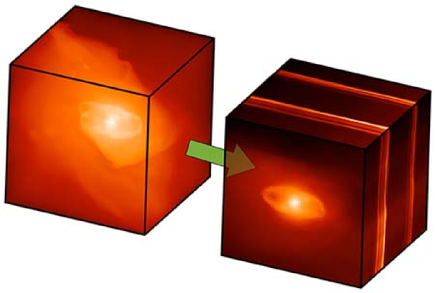
Figure 1.— Sketch of XIM process: Turn a 3D data cube of density, temperature, velocity, metallicity, and filling factor into a (2+1)D spectral data cube (shown is an IXO simulation of the iron K$\alpha$ line region of a radio galaxy like Cygnus A, see §4). The left cube is 450 kpc on a side, while the right cube has the same spatial dimensions on the x- and z-axes and spans an energy range from 6.2 to 6.8 keV on the y-axis (into the paper).

As the astronomical community considers the possibilities presented by IXO , an ultra–high resolution spectrograph with unprecedented collecting area, it is vital that we construct detailed models of what we can expect in terms of spectral line signatures from complex systems like galaxy clusters and supernova remnants. Hydrodynamic simulations and subsequent virtual observation with IXO present one of the best ways to explore the incredible wealth of information such data will offer.

Given that no observatory with anywhere near as good a spectral resolution, let alone combined with the planned large area nd and high angular resolution, has ever successfully flown, experience from past X-ray missions is clearly limiting our imagination, and more sophisticated tools will be necessary to properly plan for the advent of IXO .

At the same time, long Chandra observations of diffuse objects can benefit greatly from prior numerical simulation and it is generally recommended that observers perform ray-tracing simulations when proposing long observations. XIM can perform such simulations and presents a powerful tool in constructing mock Chandra observations of possible targets.

This paper is organized as follows: In §2, we will describe the computational details of how XIM converts input data into virtual X-ray observations, while §3 presents some examples of how XIM could be used and a brief discussion of some of the limitations inherent in XIM . Section 4 presents a brief summary.

2. Implementation and algorithms

In this section, we will describe the X–ray imaging pipeline XIM. XIM consistst of a suite of publically available IDL programs that automate the creation of simulated X-ray data for a range of satellites, with a particular focus on simulations of Chandra and IXO observations.

It takes input from hydro simulations of astrophysical objects with a focus on galaxy cluster– and cosmological simulations. Combined with a catalog of hydro or MHD simulations, it can thus be easily made into a virtual observatory that can be scripted and operated remotely (e.g., via a web interface).

In the following we describe in sequence the steps taken by XIM towards a virtual X-ray observation.

2.1. Data input

XIM is directly suited for grid-based hydro simulations. All input must be gridded on rectilinear grids. Adaptive mesh refinement (AMR) is only possible in the sense of staggered meshes, not yet in the sense of completely independent cell sizes.

The main input variables for XIM are the particle density, the gas temperature, and the gas velocity in the form of three dimensional arrays. Additionally, XIM can accept arrays of metal abundance (relative to solar) and volume filling factor of the emitting gas (these variables can also be be passed as scalars, in which case they will be applied to the entire simulation).

In addition, physical coordinate vectors (and optional telescope pointing, roll angle, and off-set parameters) are used to calculate the emitting volume and angular size of each volume element of the input data, given an object red-shift and cosmology. By default, XIM uses concordance cosmological parameters of $H_{0}=70\,{\rm km/s}$, $\Omega=1.0$, $\Omega_{\Lambda}=0.7$, $\Omega_{\rm matter}=0.3$.

The simulation output is calculated on a user specified energy grid, which can be set to correspond one–to–one to the energy channel mapping of the instrument. This allows the user to easily create full resolution spectra as well as multi-color images, or low-resolution spectra for reduced computational expense (high resolution spectra at IXO resolution can be very costly to run). A uniform turbulent velocity broadening can be applied to the spectrum to simulate sub-grid effects. A uniform foreground hydrogen column density can be specified for photo-electric absorption.

2.2. Spectral models

2.2.1 Thermal spectral calculation

By default, XIM uses the publically available APEC model to calculate spectra from thermal plasma emission (assuming gas in coronal equilibrium) for each cell (Smith et al., 2001a). APEC self–consistently calculates the equilibrium ionization balance for a thermal plasma. Atomic data are taken from the ATOMDB using APED (Smith et al., 2001b) and combined with bremsstrahlung continuum for all species. APEC output is provided as a table of spectral models.

Given the fact that APEC itself provides a table of model spectra, and given that the computational expense of extracting a spectrum from APEC is high, the most economical method of calculating a large number of spectra with XIM is by creating an oversampled table of model spectra for the entire temperature range spanned by the simulation. Thus, the spectral projection in XIM is based on interpolation on a table of model spectra, on a logarithmic temperature and photon energy grid (see §2.3).

The default temperature binning of the table is 66 bins per decade in temperature (significantly oversampled with respect to the APEC model output and sufficient for high-accuracy spectral interpolation, again see §2.3).

Two sets of spectral tables are created: One for Helium and Hydrogen, assuming primordial cosmic Helium abundance, and one for heavier elements (with relative abundance of metals fixed to the solar ratios). The metal abundance $Z$ can be specified for each cell. A model grid at default Chandra resolution is shown in Fig. 2.

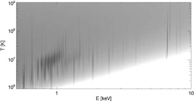
Figure 2.— Twodimensional image of a model grid at default XIM resolution for Chandra simulations, as function of gas temperature and photon energy, for solar abundance, as calculated from APEC .

2.2.2 Other spectral models

XIM is not limited to the implementation of APEC described above for spectral modeling. Any user-defined spectral model can be applied (e.g., simple powerlaw spectra) and an arbitrary set of spectral parameters and input data can be passed.

However, because XIM is optimized for thermal emission, the spectral model must be such that the emission is proportional to some power of a density variable (this could be relativistic electron pressure, which enters synchrotron emission as the 7/4 power) and a temperature variable (which controls the spectral shape and normalization, e.g., synchrotron age).

The output spectra must be provided in the form of a two-dimensional table in temperature and photon energy with logarithmic spacing on the energy axis

2.2.3 Foreground absorption

XIM allows the specification of the neutral Galactic hydrogen column density to calculate photo-electric foreground absorption following the Wisconsin Absorption Model (WABS Morrison & McCammon, 1983).

2.3. Spectral projection

The spectral projection along the line of sight is performed along an arbitrary viewing angle. For each cell of the input data, a unique spectrum is calculated for the cell temperature, cell density, and its proper Doppler shift, given the line–of–sight velocity of that cell.

To project along an arbitrary line–of–sight, the input data arrays are rotated (using tri-linear interpolation) onto a new grid that orients the x-axis along the line–of–sight vector. The input velocity arrays are also projected onto the line–of–sight vector to calculate a line–of–sight velocity for every cell. Line–of-sight integration then simply proceeds along the x-axis of the new array.

2.3.1 Doppler shift and energy gridding

The Doppler frequency correction from the emitting to the observed frame is

$$\nu_{\rm obs}=\delta\nu_{\rm emit}={\nu_{\rm emit}}\sqrt{\frac{1-v_{\rm LOS}/c}{1+v_{\rm LOS}/c}}$$ (1)

If the frequency grid is logarithmically spaced, Doppler shift is a simple addition. This suggests that spectral calculations should be performed on logarithmic grids, which is the model adopted by XIM . On a logarithmic energy grid, Doppler shift is a simple linear shift along the grid, which is computationally trivial.

Thus, given an output energy grid (either user–defined or fixed to the instrument channel map), XIM creates an over–sampled logarithmically spaced energy grid that is padded on both sides by the maximum Doppler shift encountered in the input data and takes into account the energy resolution of the instrument, additionally extending the grid to enclose a minimum of 99% of the energy at the grid edge.

The energy resolution of the logarithmic grid is set to oversample the target output grid by at least a factor of 2. Since the energy grid used by XIM is logarithmic, most of the energy range is oversampled by a larger factor.

Doppler shift is performed by linear interpolation between the nearest two integer shifts along the energy axis that straddle the actual Doppler shift value of each cell. This accurately reproduces the mean line centroid energy and leads to a small error in line width that is well below the energy bin width and well below the intstrument resolution.

The accuracy of this procedure is demonstrated in Fig. 3, which shows the line centroid energy determined by XSPEC for a gaussian spectral line with varying Doppler shift virtually observed with IXO (to sufficiently high signal–to–noise to eliminate statistical error).

Figure 3.— Accuracy of the numerical Doppler shift procedure relative to the actual Doppler shift. Shown are XSPEC fits to the line centroid (dots) for a range of Doppler shifts applied to the gaussian line and then virtually observed with IXO (actual Doppler shifted centroid energy shown as solid line). The centroid is determined to very high accuracy. Also shown are the IXO energy resolution of 2.5 eV and energy channel width of 0.5 eV.

2.3.2 Line–of–sight integration

In addition to the Doppler shift correction, the line–of–sight integration must interpolate the spectral model for each cell from the table provided by the spectral model calculation described in §2.2.

This is done by linear interpolation between the two nearest temperature spectra in the model table. Given the default dense sampling of the spectral model grid (66 temperature bins per temperature decade), this method provides a smoothly varying, accurate description of the spectra as a function of cell temperature.

Given both temperature and Doppler calculations, the line–of–sight integration is then performed on a cell–by–cell basis. For an input grid of size $N_{x}\times N_{y}\times N_{z}$ and a logarithmic energy grid with $N_{\rm le}$ bins, this involves $N_{x}N_{y}N_{z}N_{\rm le}$ calculations, which can be very time consuming and lends itself to trivial parallelization. A simple implementation of parallelization of this step is included in XIM .

The line–of–sight integration is performed before re-gridding to the instrument pixel scale to preserve the maximum amount of velocity detail from the original hydro simulation. However, for high-resolution spectra, as encountered with IXO , memory requirements can become extreme. In some cases, it is therefore advisable to re-sample the input grid to lower resolution, appropriate for the lower angular resolution of the telescope (however, this procedure will lead to an under-estimate of the Doppler width of the lines).

To keep memory requirements at a minimum, spectra are accumulated on a pixel–by–pixel basis (i.e., the line–of–sight integration is performed along the line of sight first, then across the image). Thus, only the input data and the spectral cube of dimension $N_{x}N_{y}N_{\rm le}$ have to reside in memory.

2.4. Virtual observation

The output from the line–of–sight projection encapsulates the object’s cosmological red-shift, but it is still instrument–indepent (though often the energy grid will be chosen to be suitable to a particular instrument to keep computational expense and memory requirements at a reasonable level; e.g., for virtual Chandra observations, emphasis should be placed on spatial resolution, while for virtual IXO obsevations, the energy grid should be at the highest resolution possible).

Starting from the output file of the line–of–sight inegration, virtual observations with different target telescopes and instruments are performed in a number of steps described below.

2.4.1 PSF simulation

The line–of–sight integrated spectral cube is convolved with the telescope point spread function (PSF). XIM allows user specified PSF models. Note that off-axis effects on the PSF and vignetting are currently not included in XIM , i.e., it is assumed that the PSF is uniform across the field–of–view.

The default PSF used for IXO simulations was extracted from the IXO simulator simx, which provides a monochromatic PSF (specified at 6keV).

The default PSF for Chandra simulations was extracted from MARX ray–tracing simulations and is interpolated in energy with a native spacing of 0.5 keV. The low-energy resolution is 0.5 arcseconds (see Chandra users guide for more information on the energy dependence of the PSF). More accurate Chandra imaging simulations, including vignetting and off-axis effects, can be achieved using the optional MARX interface described in §2.4.5.

2.4.2 Convolution with instrument responses

A critical component of realistic X-ray simulations is the incorporation of the effective area of the telescope as a function of photon energy (encapsulating mirror effective area and detector quantum efficiency, typically encoded in the ancillary response file in X-ray astronomy) and the redistribution function of photon energy (reflecting the spectral resolution of the telescope and detector, typcially encoded in the response matrix file). This happens in three steps:

• Given a response file (following the CAL/GEN/92-002 FITS specifications), XIM either re-grids the telescope response to the logarithmic energy bin on the data energy axis and the user-supplied output energy grid on the the detector axis, or, if XIM uses native telescope energy channels, the line–of–sight projection is re-gridded from logarithmic onto detector channels.

• Next, the line–of-sight projected, PSF–convolved data cube is re-gridded onto physical detector pixels for the specified telescope/detector.

• Finally, XIM convolves the spectral cube with the instrument response onto the specified output energy grid, resulting in a spectral cube of count rates per energy bin per pixel as detected by the instrument.

2.4.3 Virtual detection

XIM assumes Poisson noise for counting statistics and produces an IDL data file that includes the detector count rate (without statistical error) and a counts file for the user-specified exposure time that includes Poisson errors.

In addition to IDL output, XIM can produce a FITS events file that can be analyzed with standard X-ray astronomy tools like ftools and ds9 .

XIM can also produce a single FITS spectrum for the entire observation. Post-processing with the spectral generator of XIM allows the application of IDL mask arrays to select sub-regions of the spectrum (or select different weighting for different pixels for the combined spectrum) and produce FITS spectra that can be analyzed with XSPEC , isis , and sherpa . It is possible to create multiple different spectral files for different regions from the same ximulation (e.g., annuli around a cluster center for deprojection analysis).

2.4.4 Backgrounds

XIM adds sky background and instrumental background to the virtual observation. These can be user-specified spectra or standard background estimates included for Chandra and the IXO calorimeter XMS.

Sky background is treated like source photons and is folded through the instrument response (though assumed to be uniform across the field–of–view, so no PSF convolution is performed). Instrument background is added directly to the output counts without convolution with the response.

The default background for Chandra was extracted from the black sky background file for post-2000 data. The IXO background estimate is based on the most recent estimates available on the telescope wiki page and will be continually updated as more sophisticated estimates become available.

2.4.5 Virtual Chandra observations with MARX

XIM comes with default Chandra observing parameters (the latest aimpoint response files should be downloaded by the user from the Chandra web archive). This alows high-fidelity simulations of objects near the aimpoint.

However, for observations of objects far off-axis, PSF effects and vignetting should be taken into account. Thus, for the most realistic virtual Chandra observations, XIM uses MARX (the official Chandra simulation software) to perform ray-tracing simulations of the observation. The output is again a fully compliant Chandra FITS events file that can be analyzed using ciao and the Chandra pipeline like regular Chandra data.

3. Discussion

Having briefly described the steps taken by XIM to convert a grid of data taken from a hydro simulation into a virtual X-ray observation, we will present some examples of possible applications (the details of which will be presented in a separater paper) and discuss some of the limitations.

3.1. Examples of applications

3.1.1 Chandra imaging of radio galaxies in clusters

Before going into more detail, we list several examples of possible applications of XIM for Chandra :

• A good demonstration of the power of X-ray imaging is the unsharp–masked image of the Perseus cluster (Fabian et al., 2003) that shows a series of concentric ripples (identified as sound waves and a weak shock). While direct one–to–one simulations of a Perseus are not possible given the difficulty in reproducing the details in cluster weather that likely lead to the asymmetric appearance of the cluster, it is nonetheless very usefull to examine hydro simulations for whether they can reproduce the observed surface brightness fluctuations induced by these waves.

• X-ray astronomy makes use of object colors for selection effects. For example, (Forman et al., 2007) used a color cut on a long Chandra observation of the Virgo cluster to detect a weak shock driven into the cluster by the radio galaxy M87 at the center.

• As a further example, a cosmological simulation containing multiple galaxy clusters can be examined for the optical set of bands within which to select galaxy clusters, depending on the instrument used.

Multi-color imaging is particularly easy and fast using XIM , given that only a small number of spectral channels have to be calculated (APEC calculates the integrated photon luminosity for a given energy band, so no interpolation is involved when calculating broad band images).

Fig. 4 shows the simulated Chandra surface brightness and the unsharp-masked image for a hydro simulation of Cygnus A. The details of the hydrodynamical simulation are described in Heinz et al. (2006) and we limit this discussion to a very brief summary of the features of this simulation: We used the publically available FLASH code (Fryxell et al., 2000) to simulate the injection of a super-sonic, powerful jet into a galaxy cluster (taken from (Springel et al., 2001)). The jet power ($10^{46}\,{\rm ergs\,s^{-1}}$) and the cluster temperature ($\sim 5\,{\rm keV}$) and central density match the canonical parameters for Cygnus A very well (e.g., citepwilson:02). When placing the simulated cluster at the red-shift $z=0.0561$ of Cygnus A (picking a time step that reproduces the observed angular sizes of the X-ray cavities and the shock in Cygnus A) the simulated Chandra surface brightness is in good agreement with the actual Chandra observation (to within about 10%).

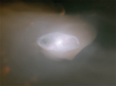
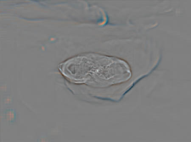
Figure 4.— Simulated Chandra image of Cygnus A (top) and unsharp-masked version of the same image (bottom). Three colors correspond to 0.5-2.0 keV (red), 2.0-5.0 keV (green), and 5.0-10.0 keV (blue). The image x and y dimensions are 440 x 330 kpc. The unsharp-masked image clearly shows ripples reminiscent of those seen in, for example, Perseus A. Note that the images shown are calculated with infinite signal–to–noise to demonstrate the appearance of ripples in X-ray images behind shock waves. Given a proper exposure time, it would be trivial to determine the detectability of features at a given surface brightness.

The power and importance of virtual X–ray imaging can be demonstrated from the unsharp–masked image: The appearance of ripples in the wake of the outgoing shock wave is clear from this image. It implies that X-ray surface brightness ripples can be excited in the wake of one single outgoing shock wave as a result of jet dynamics and do not necessarily require multiple episodes of activity of the central radio galaxies.

Given the abundant data on X–ray cavities in clusters in the Chandra archive, a statistical treatment of bubble properties has now become possible. When computing the observability and imaging properties of a sample of bubble either from simulations or analytic models, it is critical to employ faithful rendering of the virtual X-ray data. Using XIM , Brueggen et al. (2009) have demonstrated the importance of line–of–sight projection for estimating bubble position and size from observations.

3.1.2 High-resolution IXO spectroscopy of a virtual clone of Cygnus A

Using the same hydro simulation described in §3.1.1, we used XIM to simulate a high–resolution spectrum of a powerful radio galaxy like Cygnus A observed with IXO . A more detailed description of the power of high–resolution spectroscopy for the study of radio galaxies will be published in a companion paper. Here we wish to demonstrate the power of such observations using a simple example.

The high spectral resolution of IXO will allow detailed kinematic mapping of the expanding cavities of radio galaxies. Figure 5 shows three spectra, one through the cluster center and two through the expanding cavities. The line emission is due to the K-$\alpha$ lines from FeXXV and FeXXVI (Helium– and Hydrogen–like iron), which emit abundantly in hot cluster atmospheres like that of Cygnus A.

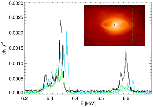
Figure 5.— Simulated IXO spectra of Cygnus A for three lines of sight (green/yellow: through the left cavity; black: Through the cluster center; cyan: Through the right cavity). The three most prominent peaks of the cyan spectrum show the approaching and receding cavity walls, as well as the cluster fore- and background emission. The offset relative to the cluster emission (black) is due to some rotation in the cluster and the jet inclination relative to the line of sight. The image inset shows the simulated image of the cluster.

The two spectra taken through the cavity centers show clear evidence for Doppler-shifted line emission from the front and back walls of the cavity and it is possible to simply read off the expansion velocity from the spectrum to be $614\,{\rm km\,s^{-1}}$ from the separation of the three right-most peaks of the cyan spectrum. These three peaks are all due to the resonance line of FeXXV from the rear wall (left peak at $6.341\,{\rm keV}$), the front wall (right peak at $6.367\,{\rm keV}$) and the fore– and background cluster emission (middle peak at $6.354\,{\rm keV}$). The expansion line–of–sight velocity in the simulation is $v_{\rm shell}\approx 650\,{\rm km\,s^{-1}}$.

More sophisticated model fitting would allow us to determine the emission measure distribution at different velocities, possibly allowing a deconvolution of the internal dynamics of the shell (which is not moving at uniform velocity). This could be used to, for example, determine the rate at which gas is flowing back along the shell as well as detecting the creating of high entropy gas around shells as direct evidence of heating and feedback.

Other obvious examples of using high-resolution X-ray spectroscopy in the context of galaxy clusters include detailed APEC model fits to determine the temperature and metallicity distribution of the cluster gas. Demonstrations of the power of this method are beyond the scope of this paper, but the XMM-Newton obervations of galaxy clusters that gave rise to the second cooling flow problem (ultimately leading to the current paradigm of AGN heating of clusters) provide evidence of the power of this method (Peterson et al., 2003) even at the lower resolution and throughput of XMM-Newton .

It is also possible to incorporate and test multi-phase models versus observations. This can be easily achieved by super-imposing multiple XIM simulations (one for each phase).

3.2. Limitations

Finally, we will briefly discuss some of the current limitations on the software that are not likely to be remedied or implemented in the near future.

3.2.1 Grid geometries

Based on the projection method, the code can only handle input data on regular grids that can be described by a single, rectungular three dimensional matrix. This excludes true AMR grids (though it allows for staggered grids) and, naturally, Lagrangian formulations from direct application. To use XIM with AMR or SPH output data, they will have to be re-gridded onto a regular grid. The same is true for non-cartesian grids. The examples shown above were all calculated with the AMR code FLASH and then re-gridded onto a regular cartesian grid.

3.2.2 Line–of–sight projections

Direct integration along the coordinate axes is computationally simpler and faster, which is the method employed by XIM . This implies that all input arrays have to be rotated prior to the spectral projection. As with regular projections through a rectangular volume for arbitrary line–of–sight vectors, missing values lead to the appearance of projection effects (e.g., the volume is rendered as a projected box. Currently, XIM does not allow for period boxes to be rendered without data loss. It is possible to clip the data, however, to avoid the appearance of projection artifacts from missing values.

3.2.3 Spectral models

As already described, XIM incorporates the APEC thermal plasma emission code for plasma in coronal equilibrium. The method used to interpolate spectra assumes that the spectral shape depends only on one parameter (the temperature or an equivalent variable that can be passed instead of temperature) and that the emissivity is proportional to the square of the density (or to some power of an equivalent variable that can be passed instead)

XIM allows user-defined spectral models as long as they can be written in such a way that they depend on two parameters (one that determines the spectral shape, such as temperature and one that affects the normalization through a powerlaw dependences). As long as this is the case, it is straight forward to incorporate other models. For example, synchrotron emission could be included by having the spectral shape (index and/or cutoff) determined by one parameter (which is passed as the variable t, but could in fact be the spectral age of the plasma) and the overall normalization is determined by the non-thermal pressure (which would be passed as the parameter n). Spectral shifts would be incorporated through the line–of–sight velocity v.

Clearly, this method is somewhat limiting in the way that spectral models can be formulated. For example, photo-ionized plasmas will be difficult to implement.

3.2.4 Imaging restrictions: Vignetting and off-axis

As already mentioned above, XIM assumes a uniform PSF across the field–of–view and neglects vignetting. For IXO , these extent of these effects is currently not well known. For Chandra , the best way to incorporate these effects is to use the MARX option to pipe the spectral cube through the telescope ray tracing software. This will produce the most realistic Chandra simulations.

4. Conclusions

We have presented a description of the public code XIM . The code produces virtual X-ray observation from hydro simulation of astrophysical plasmas. The code is best suited for the simulation of thermal emission, using the APEC model. XIM incorporates detailed telescope parameters and responses for Chandra and IXO . Examples of the application for XIM include multi-color imaging, detailed surface–brightness mapping (e.g., using unsharp–masking), high-resolution kinematic studies of the dynamics of galaxy clusters, groups, and supernova remnants, and multi-temperature, multi-phase high resolution spectroscopy of space plasmas. Current limitations include the restriction to regular, rectangular grids, spectral models that can be parameterized in a fashion equivalent to thermal emission, and restriction to on-axis imaging performance.

References

- Brueggen et al. (2009) Brueggen, M., Scannapieco, E., & Heinz, S. 2009, MNRAS, accepted
- Fabian et al. (2003) Fabian, A. C., Sanders, J. S., Crawford, C. S., Conselice, C. J., Gallagher, J. S., & Wyse, R. F. G. 2003, MNRAS, 344, L48
- Forman et al. (2007) Forman, W., Churazov, E., Markevitch, M., Nulsen, P., Vikhlinin, A., Begelman, M., Boringer, H., Eilek, J., Heinz, S., Kraft, R., & Owen, F. 2007, ApJ, 665, 1057
- Fryxell et al. (2000) Fryxell, B., Olson, K., Ricker, P., Timmes, F. X., Zingale, M., Lamb, D. Q., MacNeice, P., Rosner, R., Truran, J. W., & Tufo, H. 2000, ApJS, 131, 273
- Heinz et al. (2006) Heinz, S., Brüggen, M., Young, A., & Levesque, E. 2006, MNRAS Letters, 373, 65
- Morrison & McCammon (1983) Morrison, R. & McCammon, D. 1983, ApJ, 270, 119
- Peterson et al. (2003) Peterson, J. R., Kahn, S. M., Paerels, F. B. S., Kaastra, J. S., Tamura, T., Bleeker, J. A. M., Ferrigno, C., & Jernigan, J. G. 2003, ApJ, 590, 207
- Smith et al. (2001a) Smith, R. K., Brickhouse, N. S., Liedahl, D. A., & Raymond, J. C. 2001a, ApJ, 556, L91
- Smith et al. (2001b) Smith, R. K., Brickhouse, N. S., Liedahl, D. A., & Raymond, J. C. 2001b, in Astronomical Society of the Pacific Conference Series, Vol. 247, Spectroscopic Challenges of Photoionized Plasmas, ed. G. Ferland & D. W. Savin, 161
- Springel et al. (2001) Springel, V., White, M., & Hernquist, L. 2001, ApJ, 549, 681