Master Equation and Control of an Open Quantum System with Leakage

Abstract

Given a multilevel system coupled to a bath, we use a Feshbach $P,Q$ partitioning technique to derive an exact trace-nonpreserving master equation for a subspace $\mathcal{S}_{i}$ of the system. The resultant equation properly treats the leakage effect from $\mathcal{S}_{i}$ into the remainder of the system space. Focusing on a second-order approximation, we show that a one-dimensional master equation is sufficient to study problems of quantum state storage and is a good approximation, or exact, for several analytical models. It allows a natural definition of a leakage function and its control, and provides a general approach to study and control decoherence and leakage. Numerical calculations on an harmonic oscillator coupled to a room temperature harmonic bath show that the leakage can be suppressed by the pulse control technique without requiring ideal pulses.

Introduction.— Control of quantum dynamics is of great interest for “quantum technology industries”, such as quantum computing. The control of closed quantum systems is well established, and has been extensively studied in areas such as chemical physics Brumer02 ; Rice . Efforts to extend these studies to open systems, where the system interacts with an environment, are now underwayWuBrumer . Quantum information processing has already expended considerable effort on open systems. Hence, we anticipate that methods being developed in the latter area may well be useful in the former, and vice-versa Betal .

A fundamentally difficult problem in quantum information processing is that of decoherence, i.e., the loss of quantum information in a system due to its interaction with its environment (or “bath”) Nielsen00 ; Kempe01 . For multi-level systems, such as molecules, the interaction can also cause leakage (i.e. loss of population) from a system subspace of interest, denoted $\mathcal{S}_{i}$, into the system space outside of $\mathcal{S}_{i}$. Theoretical strategies for combating such deleterious environmental effects in the absence of natural decoherence free subspaces Kempe01 ; Zanardi97 , invoke the dynamical control of system-environment interactions by external fields Viola98 ; Agarwal99 ; Wu020 ; Lloyd00 ; Lidar05 ; Kurizki04 ; Alicki-etal .

The aim of dynamical control in open systems is to suppress effects of the environment in order to control system processes at will. For example, ideal Bang-Bang (BB) control of decoherence, decay and leakage Wu020 ; Lloyd00 utilizes idealized zero-width pulses and the Trotter formula to achieve this goal, although higher-order finite-pulse widths have been considered in model cases Lidar05 .

Proposals to control decoherence by realistic (non-ideal) pulses have often invoked Zwanzig’s projection operator techniques Kurizki04 ; Alicki-etal resulting in a differential master equation for the density operator of the system up to second order in the system bath coupling. This equation allows the tractable treatment of complicated quantum dynamical processes, eliminating the ideal zero width pulses and Trotter formula assumptions and allowing natural dynamical evolution and dynamical control on an equal footing. For example, Ref. Kurizki04 provides a unified way to suppress the decoherence of two level systems by arbitrary fields that control the system-bath interaction.

Below, we consider an $N$ dimensional system ($N$ can be infinite), spanned by the bases $\left\{\left|n\right\rangle\right\}$, coupled to a bath, and develop procedures to protect quantum information stored in a $d$-dimensional subspace $\mathcal{S}_{i}$ of the system. Specifically, we use a projection operator approach to obtain an exact trace-nonpreserving master equation for the dynamics of the system subspace $\mathcal{S}_{i}$. We then introduce a characteristic leakage function which is used to consider dynamics and control of this subspace to second order in the system-bath interaction.

Zwanzig’s Projection-Operator Approach.— The most general Hamiltonian of the $N$ dimensional system plus the bath is

$$H=H_{0}+H_{I}=H_{S}+H_{B}+H_{I},$$ (1)

where $H_{S}$ and $H_{B}$ are the system and bath Hamiltonians, respectively, and the system-bath interaction is $H_{I}=\sum_{\alpha}S_{\alpha}B_{\alpha}$, where $S_{\alpha}$ and $B_{\alpha}$ are Hermitian system and bath operators. During the dynamics, the information stored in the system subspace of interest $\mathcal{S}_{i}$ will distribute into the bath and leak into the system states outside of $\mathcal{S}_{i}$ if one does not protect the subspace. Therefore, in order to store the information in $\mathcal{S}_{i}$, we need to control the system through an interaction with an external field $H_{c}(t)$, protecting the information during the course of time $t$. The total system Hamiltonian including control is therefore $H_{S}(t)=H_{S}+H_{c}(t)$.

We first derive a closed master equation for $\mathcal{S}_{i}$. Since $\mathcal{S}_{i}$ opens both to bath and to other system states outside of $\mathcal{S}_{i}$, effects of leakage have to be considered in deriving a master equation. As usual, the derivation begins in the interaction representation with respect to $H_{0}$, in which the equation of motion is $\frac{\partial}{\partial t}\,\rho(t)=-i[H_{I}(t),\rho(t)]\equiv\mathcal{L}(t)\rho(t)~{}$. Here the system-bath interaction is $H_{I}(t)$ in the interaction representation and the Liouville superoperator $\mathcal{L}(t)$ is defined by this equation Breuer02 . The superprojection operation $\mathcal{P}$ that we seek defines the relevant part of the total density matrix Breuer02 $\mathcal{P}\rho(t)$ for our new open system, i.e. the subspace $\mathcal{S}_{i}$ of the entire system. Specifically, the superprojection operation comprises two commuting parts: a trace over the bath components, and a projecting out of the $\mathcal{S}_{i}$ subspace from the full $N$-dimensional space of the system. The associated superprojector $\mathcal{P}$ is therefore defined as

$$\mathcal{P}\rho=\mathbf{P}\text{ tr}_{B}\{\rho\}\mathbf{P}\otimes\rho_{B}\equiv\eta\otimes\rho_{B},$$

where $\mathbf{P}=\sum_{i=0}^{d-1}\left|i\right\rangle\left\langle i\right|$ denotes a projection onto $\mathcal{S}_{i}$ and $\eta$ is the relevant part of the total density matrix, which is projected from the total system density matrix $\rho_{S}=$ tr${}_{B}\rho$ as $\eta\equiv\mathbf{P}\rho_{S}\mathbf{P}$. The matrix $\rho_{B}$ is chosen as the initial state of the bath. The trace of the matrix $\eta$ is not necessarily one, but $\eta$ satisfies a closed equation as does $\rho_{S}$, and plays the same rule as $\rho_{S}$, but in $\mathcal{S}_{i}$. That is, an arbitrary system observable acting only on $\mathcal{S}_{i}$ obeys the relation $O=\mathbf{P}O\mathbf{P}$. The expectation value of the operator $O$ when the system+bath is in state $\rho$ is tr$\{\rho O\}=$tr$\{\mathbf{P}\rho_{S}\mathbf{P}O\}=$tr$\{\eta O\}$, which is the same as the expectation value of the operator $O$ in the state characterized only by $\eta$. This implies that the matrix $\eta$ provides a complete description of the physics in $\mathcal{S}_{i}$, in the same sense that $\rho_{S}$ completely describes the total open system.

Applying the superprojector to the equation of motion for $\rho$ gives a time-local master equation

$$\frac{\partial}{\partial t}\,\mathcal{P}\rho(t)=\mathcal{K}(t)\mathcal{P}\rho(t),$$ (2)

where $\mathcal{K}(t)$ is the time-convolutionless generator Breuer02 . Unlike the usual approach, our new system is a $d-$dimensional subspace of the $N$-dimensional space of the total system. Alternatively, Eq. (2) can be derived by applying the Feshbach projection operator approachShore ; Rice2 to the traditional trace-preserving master equation for $\rho_{S}$.

Equation (2) is exact and holds for almostBreuer02 all arbitrary systems and interactions, and for initial conditions $\rho(0)=\mathcal{P}\rho(0)$, i.e. where the quantum system is initially within $\mathcal{S}_{i}$. Since population can flow out of this subspace, the master equation is not trace-preserving. Unfortunately this equation is as difficult to solve as the original equation. Therefore, perturbation expansions are needed in order to apply the result to actual problems.

To second order in the coupling strength of the interaction, $\mathcal{K}(t)=\int_{0}^{t}ds\mathcal{PL}(t)\mathcal{L}(s)\mathcal{P}$. Introducing the explicit expressions for the projection operator and the Liouville superoperator, we can obtain the second-order $d\times d$ dimensional master equation in the interaction representation,

$$\frac{\partial}{\partial t}\,\eta(t)=-\lambda^{2}\int_{0}^{t}ds\mathbf{P}\text{ tr}_{B}[H_{I}(t),[H_{I}(s),\eta(t)\otimes\rho_{B}]\mathbf{P}.$$ (3)

Here $\lambda H_{I}$ replaces $H_{I}$, with the small parameter $\lambda$ introduced to characterize the order of perturbation expansion. For the single component interaction $H_{I}(t)=S(t)B(t)$, Eq. (3) can be considerably simplified.

One Dimensional Dynamics and the Principle of Control.— A primary example is the dynamics, control and protection of one normalized state $\left|\phi\right\rangle$, in the interaction representation, within the $d-$dimensional subspace $\mathcal{S}_{i}$. [Spontaneous emission, for example, is a case where $\left|\phi\right\rangle$ is an energy eigenstate]. In general $\left|\phi\right\rangle$ is a superposition of eigenstates, rather than a single eigenstate, and we can rearrange the bases of $\mathcal{S}_{i}$ so that $\left|\phi\right\rangle$ is one of the new orthonormal basis elements.

Suppose that the initial state $\eta(0)=\left|\phi\right\rangle\left\langle\phi\right|$. The subsystem evolves according to the closed equation (3) with $d=1$ and, at time $t$, $\eta(t)=b(t)\left|\phi\right\rangle\left\langle\phi\right|$, where, in general, $b(t)$ is written as

$$b(t)=\exp(-L(t)),$$ (4)

with $b(t)\leq 1$ or $L(t)\geq 0.$ Substituting $\eta(t)$ into the master equation (3) with $d=1$, gives an analytic expression second order in $\lambda$,

$$L(t)=\lambda^{2}\int_{0}^{t}dsC(s),$$ (5)

where

$$C(s)=\int_{0}^{s}ds^{\prime}\sum_{\alpha\beta}[\mathfrak{S}_{\alpha\beta}(s,s-s^{\prime})\Phi_{\alpha\beta}(s^{\prime})+h.c.],$$ (6)

and $\mathfrak{S}_{\alpha\beta}(s,s^{\prime})=\overline{\Delta S_{\alpha}(s)\Delta S_{\beta}(s^{\prime})}$ . Here $\Delta S_{\alpha}(t)=S_{\alpha}(t)-\overline{S_{\alpha}(t)}$ and $\overline{S_{\alpha}(t)}=\left\langle\phi\right|S_{\alpha}(t)\left|\phi\right\rangle$. $\Phi_{\alpha\beta}(t-s)=$tr${}_{B}[B_{\alpha}(t)B_{\beta}(s)\rho_{B}]$ is the bath correlation function for multi-term system-bath interactions. Note that $C(s)$ is a linear function of matrix elements $\Phi_{\alpha\beta}$. We term the time-dependent $L(t)$ a leakage function, by analogy with the decoherence function Breuer02 . It describes the leakage from $\mathcal{S}_{i}$ due to the bath and into the space outside of $\mathcal{S}_{i}$. Higher than second order effects in the leakage function are included in Eq.(2)

$L(t)$ is a functional of the initial state $\left|\phi\right\rangle$ and any added control $H_{c}$, the latter generally through incident external fields. Given a time $t$, the solution of the variational equation $\delta L(t)=0$ with respect to the state $\left|\phi\right\rangle$ in the absence of $H_{c}$ yields, to second order, a self protected state. Alternatively, solution to this variational equation with respect to the incident electromagnetic fields for fixed $\left|\phi\right\rangle$ provides optimal control fields, to second order, to protect $\left|\phi\right\rangle$ against decoherence. Later in this letter we address optimizations with respect to the control fields for realistic molecular systems. Optimizations with respect to $\left|\phi\right\rangle$ are currently under study.

As in all approximation techniques, the utility of the second order approximation [Eq. (3)] is examined by comparison with exact cases. We consider two examples.

Example I: Pure leakage. Consider a pure leakage case, where the system is a one-dimensional Harmonic oscillator in which there is no system-bath interaction. The system is described by $H_{S}=\omega a^{\dagger}a$ and is polarized by the interaction $H_{I}=\lambda(a^{\dagger}+a)\otimes I_{B}$, where $I_{B}$ is the unit operator of a bath and $a^{\dagger}(a)$ is a bosonic creation (annihilation) operator for the harmonic oscillator. For the case of the ground state $\left|\phi\right\rangle=\left|0\right\rangle$, the exact solution is $b_{\text{ex}}(t)=\left\langle 0\right|\rho_{S}(t)\left|0\right\rangle=\exp(-\frac{4\lambda^{2}}{\omega^{2}}\sin^{2}\frac{\omega t}{2})$. The second-order solution [Eqs. (4) and (5)] gives the same result. When $\left|\phi\right\rangle=\left|1\right\rangle,$ the exact analytical solution $b_{\text{ex}}(t)=(1-\frac{4\lambda^{2}}{\omega^{2}}\sin^{2}\frac{\omega t}{2})^{2}\exp(-\frac{4\lambda^{2}}{\omega^{2}}\sin^{2}\frac{\omega t}{2})$, while $b(t)=\exp(-\frac{12\lambda^{2}}{\omega^{2}}\sin^{2}\frac{\omega t}{2}).$ In the superposition case of $\left|\phi\right\rangle=\frac{1}{\sqrt{2}}(\left|0\right\rangle+\left|1\right\rangle),$ $b(t)=\exp(-\frac{4\lambda^{2}}{\omega^{2}}(\sin^{2}\frac{\omega t}{2}+\sin^{4}\frac{\omega t}{2}))$ and the exact solution $b_{\text{ex}}(t)=[1-\frac{4\lambda^{2}}{\omega^{2}}(1-\frac{\lambda^{2}}{\omega^{2}})\sin^{4}\frac{\omega t}{2}]\exp(-\frac{4\lambda^{2}}{\omega^{2}}\sin^{2}\frac{\omega t}{2}).$ Their second-order expansions are all the same and are essentially equal to one another for $\frac{\lambda^{2}}{\omega^{2}}<0.1$.

Example II: Spin-bath model within the rotating wave approximation. Here the system Hamiltonian reads $H_{0}=\epsilon\sigma^{z}+\omega a^{\dagger}a$ and $H_{I}=\lambda(\sigma^{+}a+\sigma^{-}a^{\dagger}),$ where $\sigma^{\pm}=(\sigma^{x}\pm i\sigma^{y})/2$. Let $\left|\phi\right\rangle=\left|0\right\rangle$ and let the bath be in the state $a^{\dagger}\left|V\right\rangle,$ where $\left|0\right\rangle$ is the spin-down state and $\left|V\right\rangle$ is the vacuum bath state. Solving the problem exactly gives $b_{\text{ex}}(t)=1-\sin^{2}(t\sqrt{(\frac{\epsilon-\omega}{2})^{2}+\lambda^{2}})\frac{\lambda^{2}}{\sqrt{(\frac{\epsilon-\omega}{2})^{2}+\lambda^{2}}}$. The second-order solution to the master equation is $b(t)=\exp(-\frac{16\lambda^{2}}{(\epsilon-\omega)^{2}}\sin^{2}\frac{(\epsilon-\omega)t}{2})$, which agrees with the exact result in second order. They can also be shown numerically to be in good agreement when $\frac{\lambda^{2}}{(\epsilon-\omega)^{2}}<0.1$.

Quantum Control: Within the framework outlined here, the goal of quantum control becomes: given a time $t$ of interest, we computationally seek the solution of the variational equation $\delta L(t)=0$ with respect to $H_{c}$, with the inclusion of any physical constraints of the control, The result is the control functional $H_{c}(s^{\prime}).$ Note that this approach does not just optimize $C(s)$ itself at time $s$, but rather includes the history of the time evolution of $C(s).$

Although idealized BB control provides a possible mathematical solution, of $L(t)=0$, it requires unrealistic (zero-width) pulses. Hence, our focus is to replace idealized control by an approximate variational or numerical solution that minimizes $L(t)$ under realistic pulse energy and pulse width constraints.

Harmonic Oscillator coupled to a harmonic bath.- As an application of this framework, consider as the system the harmonic approximation (frequency $\Omega)$ to a Morse oscillator Wang01 ; Paul04 for, e.g., molecular iodine, which allows us to employ a simplifying symmetry. The total Hamiltonian, where the bath has $\ell$ oscillators, is $H=\Omega a^{\dagger}a+\sum_{j=1}^{\ell}\omega_{j}a_{j}^{\dagger}a_{j}+\lambda SB,$ where $B=\sum\alpha(\omega_{j})(a_{j}+a_{j}^{\dagger})$. The interaction is separable with $S(t)=e^{-i\Omega t}a+e^{i\Omega t}a^{\dagger}$ and the bath correlation function is $\Phi(t)=\sum\alpha^{2}(\omega_{j})\{[1+n(\omega_{j})e^{-i\omega_{j}t}+n(\omega_{j})e^{i\omega_{j}t}\}$ where $n_{j}=1/[\exp(\beta\omega_{j})-1]$. At low energy, I₂ vibrational motion is harmonic, with $\Omega=213.7$cm^-1 and $\alpha(\omega_{j})=\sqrt{\frac{\omega_{j}\omega_{d}(1-e^{-5})}{40\pi\ell}}$ with $\omega_{j}=-\frac{\omega_{d}}{2}\ln(1-\frac{j(1-e^{-5})}{\ell})$ , where $\omega_{d}$ is the cut-off frequency at $j=\ell$.

As an example, consider a superposition of the eigenstates of the system harmonic oscillator as the state in need of protection in a bath at room temperature. Such states would be of interest, for example, in pump-dump coherent control scenariosBrumer02 ; Rice where this is the initially pumped state. In that case one would be interested in maintaining this state over time scales of $\approx 700$ fs, the system decoherence timePaul04 .

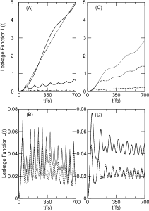
Figure 1: (A) (upper solid curve) $L(t)$ in units of $\lambda^{2}$ for an Harmonic oscillator, in the initial state, $\left|\phi\right\rangle=\frac{1}{\sqrt{2}}(\left|0\right\rangle+\left|1\right\rangle)$ coupled to a bath of 1000 harmonic oscillators at $T=$300K. Here $\omega_{d}=0.01(fs)^{-1}\approx 1.5\Omega$. The dashed curve shows the dominant part, as discussed in the text. The three lower solid curves show $L(t)$ with $\Delta=0$, $\phi_{0}=\pi$ and $\tau=\frac{\pi}{20\Omega},\frac{\pi}{10\Omega}$ and $\frac{\pi}{5\Omega}$, in the order from bottom to top. (B): $L(t)$ with $\tau=\frac{\pi}{10\Omega}$ and $\phi_{0}=\pi$, but different values of $\Delta$. Solid curve $\Delta=\tau/5;$ Dashed curve: $\Delta=\tau/2;$ Dotted curve: $\Delta=\tau.$ (C): $L(t)$ with $\tau=\frac{\pi}{10\Omega}$ and $\Delta=\frac{\tau}{2}$ but different pulse intensities, $\phi_{0}=\frac{\pi}{10},\frac{\pi}{5},\frac{\pi}{2}$ from top to bottom. (D): two lower curves, $L(t)$ with $\phi_{0}=\pi/100$, $\tau=\tau_{0}/100$ $(\tau_{0}=\frac{\phi_{0}}{10\Omega})$  and $\phi_{0}=\pi/10$ and $\tau=\tau_{0}/10$ all with $\Delta=\tau/2.$ They have the same value of $\Omega_{c}.$ The upper curves have the same values of $\phi_{0}$ and $\tau$ but different signs of $\phi_{0}$.

Figure 1A shows $L(t)$ for the parameters shown in the figure caption. In some cases, $\mathfrak{S}(s,s-s^{\prime})$ may be a function of $(s-s^{\prime})$ only, in which case $L(t)\propto t$, shown as the dashed line in Fig. 1A. This linear dependence on $t$ is similar to that of the usual decoherence function Breuer02 in the long time limit. However, at shorter times the dependence of $\mathfrak{S}(s,s-s^{\prime})$ on $s$ is seen to contribute non-negligibly, leading to oscillatory $L(t)$. Below we will numerically study the behavior of the leakage function in the short-time region to determine the extent to which leakage can be controlled.

Control.- Physically, the origin of the control is that the frequency of the system (here, an harmonic oscillator) is periodically, dynamically, Stark shifted by the alternating field. To this end we employ the realistic control Hamiltonian $H_{S}(t)=(\Omega+f(t))a^{\dagger}a$, which results from strong laser pulses acting on electrons that induce an additional time-dependent nuclear potential. We model the control function as a periodic rectangular interaction: $f(t)=0$ for regions other than $n\tau-\Delta<t<n\tau$, $n$ integer. Inside these regions $f(t)$ is defined so that $\phi_{0}=\int_{\tau-\Delta}^{\tau}f(t)dt$. That is, for nonzero $\Delta$, $f(t)=\phi_{0}/\Delta$ over the control interval, and for $\Delta=0$, $f(t)=\delta(t-n\tau)$. The functional form contains three main control parameters: the time interval $\tau$, the pulse width $\Delta$ and the interaction intensity $\phi_{0}$. For comparison with realistic pulses, we show $L(t)$ with ideal impulsive phase modulation ($\Delta=0$) in the three lower curves in Fig. 1 (A). Clearly, the shorter the control interval, the better the control.

Figure 1(B) shows $L(t)$ with fixed $\tau$ and $\phi_{0}$, but with different pulse widths $\Delta$. The results show that the quality of the control is only weakly dependent on the pulse width. For example, the control is excellent even if the width of the pulse is equal to the control interval $\tau$. In this case the control is equivalent to adding a constant frequency $\Omega_{c}=\phi_{0}/\tau$ to the harmonic oscillator frequency, i.e. shifting the system frequency by $\Delta/\tau=1$ means shifting the system frequency to ($\Omega+$ $\Omega_{c}$). If $(\Omega+\Omega_{c})>$ $\omega_{d}$ (the cut-off frequency of the bath), which is the case in this figure, the function $\mathfrak{S}(s,s-s^{\prime})$ oscillates faster than the rate of decay of the bath $\Phi(s).$ The integral, $C(s)$, of the product of the two functions generally oscillates around zero so that $L(t)$ is reduced at any time $t$. The way to achieve this goal (e.g., see Ref. Kurizki04 ) is to increase the interaction of the pulse $\phi_{0}$ or decrease the pulse width $\tau$ in order to increase $\Omega_{c}=\phi_{0}/\tau.$

The dependence on the intensity is also of interest, as shown in Fig. 1(C). The quality of control is seen to decrease with decreasing intensity.

Finally, we consider the effects due to the different signs of $\phi_{0}$. The two lower curves in Fig. 1(D) correspond to results for different $\phi_{0}$ (or $\tau$) but the same $\Omega_{c}=\phi_{0}/\tau$. The upper curves have the same values but different signs. They show similar suppression, implying that the quality of suppression depends primarily on $\Omega_{c}.$ Hence, the above discussions are also valid for the negative values of $\phi_{0}$ as shown in the two upper curves.

For the case of a diatomic molecule, we note that the AC Stark effect induced by an external laser field interacting with the electrons decreases (or increases) $\Omega$, an effect termed “bond softening (or hardening)”. Ab initio calculations Zavriyev90 show that, in the softening case, the frequency can be reduced by ten percent for H${}_{2}^{+}$ in a strong laser field. In the case of hardening, if the frequency can be enhanced by $p$ percent so that if $(1+p)\Omega>$ $\omega_{d}$, then leakage control will be effective. This is expected to be a considerable technical challenge.

Conclusion.- We have utilized an exact trace-nonpreserving master equation for dynamics of a system subspace, and introduced a leakage function that describes leakage from a subspace of interest. We used the second-order equation to analyze the quantum dynamics of the leakage function, especially for the generic case of a harmonic oscillator coupled to a bath of harmonic oscillators. The realistic pulses required to suppress leakage in the presence of the bath are given by the well studied finite-width pulses causing AC Stark shifts Kurizki04 ; Zavriyev90 . A remarkable result is that, in the one-dimensional case, one can define a leakage function that provides a complete description of quantum storage of a general superposition state $|\phi\rangle$. Since quantum storage is of great interest at present, the leakage function provides a most convenient tool for studying the control of quantum states in the short time regime relevant to quantum information processing and to coherent control.

Acknowledgement: We thank Professor Daniel Lidar for discussions with L.-A. Wu early in this work, and Goren Gordon and Noam Erez for comments and discussions. This work was supported by the NSERC Canada, a Varon Visiting Professorship to P.B. from the Weizmann Institute, the ISF and EC (MIDAS and SCALA Projects).

References

- (1) M. Shapiro and P. Brumer, Principles of the Quantum Control of Molecular Processes (Wiley-Interscience, New York, 2003).
- (2) S.A. Rice and M. Zhao, Optical Control of Molecular Dynamics (Wiley, New York, 2000)
- (3) E.g., L.-A. Wu, A. Bharioke and P. Brumer, J. Chem. Phys. 129, 041105 (2008).
- (4) P. Brumer, D. Lidar, H.-K. Lo and A. Steinberg, Quant. Info. Compu. 5, 273 (2005)
- (5) M. A. Nielsen and I. L. Chuang, Quantum Computation and Quantum Information, (Cambridge University Press, Cambridge, 2000).
- (6) J. Kempe, D. Bacon, D. A. Lidar and K. B. Whaley, Phys. Rev. A 63, 042307 (2001), and references therein.
- (7) P. Zanardi and M. Rasetti, Phys. Rev. Lett. 79, 3306 (1997).
- (8) L. Viola and S. Lloyd, Phys. Rev. A 58, 2733 (1998).
- (9) G. S. Agarwal, Phys. Rev. A 61, 013809 (1999).
- (10) L.-A. Wu, M. S. Byrd and D. A. Lidar, Phys. Rev. Lett. 89, 127901 (2002); L.-A. Wu and D. A. Lidar, Phys. Rev. Lett. 88, 207902 (2002).
- (11) L. Tian and S. Lloyd, Phys. Rev. A. 62, 05301 (2000).
- (12) K. Khodjasteh and D. A. Lidar, Phys. Rev. Lett. 95, 180501 (2005).
- (13) A. G. Kofman and G. Kurizki, Phys. Rev. Lett. 93 , 130406 (2004); G. Gordon, N. Erez, and G. Kurizki, J. Phys. B At. Mol. Opt. Phys. 40, S75 (2007)
- (14) R. Alicki, M. Horodecki, P. Horodecki and R. Horodecki, Phys. Rev. A. 65, 06210 (2002); R. Alicki, Chem. Phys. 322, 75 (2006).
- (15) H.-P. Breuer and F. Petruccione, The Theory of Open Quantum Systems (Oxford Univ. Press, Oxford, 2002).
- (16) See, e.g., B.W. Shore, The Theory of Coherent Atomic Excitation (John Wiley, N.J.,1990)
- (17) For a different approach to partitioning the system into relevant and less relevant components based upon coupling strengths using projection operators, see H. Tang, R. Kosloff and S.A. Rice J. Chem. Phys. 104, 5457 (1996).
- (18) H. Wang, M. Thoss, L. L. Sorge, R. Gelabert, X. Gimenez and W. H. Miller, J. Chem. Phys. 114, 2562 (2001).
- (19) Y. Elran and P. Brumer, J. Chem. Phys. 121, 2684 (2004).
- (20) A. Zavriyev, P. H. Bucksbaum, H. G. Muller and D. W. Schumacher, Phys. Rev. A 42, 5500 (1990); A. D. Bandrauk, ed., Molecules in Laser Fields ( Dekker, New York, 1994).