Monogamy Inequality and Residual Entanglement of Three Qubits under Decoherence

Abstract

Exploring an analytical expression for the convex roof of the pure state squared concurrence for rank 2 mixed states the entanglement of a system of three particles under decoherence is studied, using the monogamy inequality for mixed states and the residual entanglement obtained from it. The monogamy inequality is investigated both for the concurrence and the negativity in the case of local independent phase damping channel acting on generalized GHZ states of three particles and the local independent amplitude damping channel acting on generalized W state of three particles. It is shown that the bipartite entanglement between one qubit and the rest has a qualitative similar behavior to the entanglement between individual qubits, and that the residual entanglement in terms of the negativity cannot be a good entanglement measure for mixed states, since it can increase under local decoherence.

I Introduction

The behavior of entanglement in systems of many particles and the effects of decoherence on it is an important topic and far from being totally understood. If for one reason this is an issue in studying the transition from the microscopic to the classical world, it also has its practical implications since the advent of Quantum Information and Computation; a scalable quantum computer is likely to need entanglement at a many particle level.

A major obstacle in these studies is the concept of entanglement per si, as there is no established theory for multipartite entanglement (ME) and, even worse, no universal ME quantifier. One possibility is to analyse the entanglement between all possible bipartitions in the system (see Rigolin et al. (2006), for example). But even in this case there is no easy path, given that most of bipartite entanglement measures do not have an analytical expression for mixed states of systems with even small Hilbert space dimension. The Entanglement of Formation and its related quantity, the Concurrence, for example, are only exactly computable for $2\times 2$ systems (two qubits) (Wootters, 1998). An exception is the negativity, which can be obtained in any dimension (Vidal and Werner, 2002). However for Hilbert space dimension higher than $2\times 3$ it can underestimate the entanglement: it can be null when the state is entangled, defining what is called PPT entanglement or bound entanglement (two recent reviews on entanglement measures are (Plenio and Virmani, 2007; Horodecki et al., 2007) ).

Somehow related to this approach to multipartite entanglement and relevant to it is the property of monogamy: if two qubits are maximally entangled, neither of them can be entangled, in any way, with a third one (not even classically correlated${}^{\text{1}}$). But it is in the case where the two particles are only partially entangled that the monogamy property may be more relevant to multipartite entanglement. In particular, in the case of three qubits in a pure state Coffman, Kundu and Wootters (Coffman et al., 2000) obtained that $C_{A(BC)}^{2}\geq C_{AB}^{2}+C_{AC}^{2}$, with $C_{AB}$ ($C_{AC}$) being the concurrence of $A$ with $B$($C$), while $C_{A(BC)}$ is the concurrence between A and BC, with the last treated as a single system. This inequality limits A’s entanglement with B and C taken individually and do not allow both of them to increase indiscriminately, since all the quantities in the inequality varies from 0 to 1. Besides establishing this inequality Coffman, Kundu and Wootters also proposed to take the difference, $C_{A(BC)}^{2}-C_{AB}^{2}-C_{AC}^{2}$, as a tripartite entanglement measure, which they called residual entanglement, $\tau_{ABC}^{c}$. This monogamy inequality is also valid for the negativity and an analogous tripartite entanglement measure can be defined (Ou and Fan, 2007).

Even though for three particles the residual entanglement is well accepted as a tripartite entanglement measure, most of the studies of the decoherence of multipartite entanglement only focused on the bipartite part of this entanglement (Simon and Kempe, 2002; Dür and Briegel, 2004; Bandyopadhyay and Lidar, 2005; Ann and Jaeger, 2007; Montakhab and Asadian, 2008; López et al., 2008; Aolita et al., 2008) (see (Carvalho et al., 2004) and (Guhne et al., 2008) for an exception and different approach). That happens because in the case of mixed states despite the fact that the inequality and the residual entanglement can be established they involve a convex roof optimization of $C_{A(BC)}^{2}$ with no easy general solution.

Here I make use of an analytical expression for the convex roof of the pure state $C_{A(BC)}^{2}$ for rank two mixed states, obtained by Osborne (Osborne, 2005), to study the monogamy inequality and the residual entanglement under decoherence for the first time. Both are investigated in terms of the concurrence and the negativity for generalized GHZ and W states of three qubits. I also compare the behavior of the $N_{A(BC)}^{2}$ and its pure state convex roof extension.

II Monogamy and Multipartite Entanglement

One of the first investigations of the monogamy inequality and its relation to multipartite entanglement was the work of Coffman, Kundu and Wootters in 2000 (Coffman et al., 2000). There they first showed that for a pure state of three qubits

$$4\det\rho_{A}\geq C_{AB}^{2}+C_{AC}^{2},$$ (1)

with $\rho_{A}$ the reduced density matrix of the qubit $A$. To get the final inequality in terms of entanglement it is necessary to make use of two facts:

1. the concurrence of a pure state of two qubits, A and B, is given by $2\sqrt{\det\rho_{A}}$.

2. even though the state space of AB is four dimension only two of these dimensions are needed to express a pure state of ABC (this comes from the Schmidt decomposition of the state ABC in the bipartition A|BC).

Therefore A and BC can be treated as a pair of qubits in a pure state and $2\sqrt{\det\rho_{A}}$ taken as the concurrence between A and BC, obtaining the monogamy inequality

$$C_{A(BC)}^{2}\geq C_{AB}^{2}+C_{AC}^{2}.$$ (2)

This inequality allows one to define the residual entanglement as

$$\tau_{ABC}^{c}=C_{A(BC)}^{2}-C_{AB}^{2}-C_{AC}^{2}.$$ (3)

As shown in their work, the residual entanglement does not depend on which qubit is chosen as A (the focus) and can thus be considered, as remarked by the authors, as a collective property of the three qubits, that measures an essential three-qubit entanglement. The GHZ state has $\tau_{ABC}^{c}=C_{A(BC)}^{2}=1$, while a generalized W state, $\alpha|001\rangle+\beta|010\rangle+\gamma|100\rangle$, has $\tau^{c}{}_{ABC}=0$. In this way it is usually said that the W state only contains bipartite entanglement, while the GHZ state only contains genuine tripartite entanglement. Note however that both states can be considered as genuine tripartite entangled as none of them can be written in an separable way, whatever bipartition is used.

Before proceeding to the case of mixed states it is worth remarking some points which will be relevant. The concurrence of a pure state of two qubits is related to the linear entropy, $S_{L}$, of one of the sub-systems${}^{\text{2}}$

$$C_{AB}=2\sqrt{\det\rho_{A}}=\sqrt{S_{L}\left(\rho_{A}\right)}=\sqrt{2\left(1-\text{tr}\left[\rho_{A}^{2}\right]\right)}.$$

Another point that I should mention is that most of the difficulties in obtaining an entanglement measure for mixed states, comes from the fact that these are usually defined as convex roof extensions of a pure state measure. Suppose, for example, that we have a well defined measure of entanglement for pure states, $E\left(\psi\right)$. Then the entanglement of a mixed state $\rho$ is defined as

$$E\left(\rho\right)=\inf_{\left\{p_{i},\phi_{i}\right\}}\sum_{i}p_{i}E\left(\phi_{i}\right),$$

with the infimum taken over all possible decompositions of $\rho$ in a mixture of pure states, $\rho=\sum_{i}p_{i}|\phi_{i}\rangle\langle\phi_{i}|$. The concurrence of a mixed state of two qubits, for example, is the convex roof of the pure state concurrence, or equivalently, the convex roof of the square root of the linear entropy, and in the especial case of two qubits an analytical expression can be obtained.

That said, let me return to the monogamy inequality, but for mixed states. At first, when the three qubits are in mixed state $C_{A(BC)}$ is not directly defined as all the four dimensions of BC might be used. Nonetheless a convex roof extension of the squared concurrence, $\langle C_{A(BC)}^{2}\rangle^{min}=\inf_{\left\{p_{i},\phi_{i}\right\}}\sum_{i}p_{i}C_{A(BC)}^{2}\left(\phi_{i}\right)$, can be used to show that (Coffman et al., 2000)

$$\langle C_{A(BC)}^{2}\rangle^{min}\geq C_{AB}^{2}+C_{AC}^{2}.$$ (4)

From this inequality we can also define a residual entanglement for mixed states of three qubits:

$$\tau_{ABC}^{c}=\langle C_{A(BC)}^{2}\rangle^{min}-C_{AB}^{2}-C_{AC}^{2}.$$ (5)

However, in general, it will depend on which qubit was chosen as the focus. Thus for the case of mixed states it is necessary to use the average over the three possibles focus as the definition of residual entanglement, and that will be my procedure. From now on I will only use $C_{A(BC)}^{2}$ as the squared concurrence between A and BC, and when the state is mixed it is implicit that the convex roof extension was taken to obtain $C_{A(BC)}^{2}$.

The monogamy inequality can also be established for the negativity. As show by Ou and Fan in 2007 (Ou and Fan, 2007), for pure states of three qubits

$$N_{A(BC)}^{2}\geq N_{AB}^{2}+N_{AC}^{2}.$$ (6)

In the case of mixed states, despite $N_{A(BC)}^{2}$ being well definied without a convex roof procedure${}^{\text{3}}$, one has to use $\langle N_{A(BC)}^{2}\rangle^{min}$ to obtain,

$$\langle N_{A(BC)}^{2}\rangle^{min}\geq N_{AB}^{2}+N_{AC}^{2}.$$ (7)

Likewise the case of the concurrence Eq. 7 allows the definition of a residual entanglement in terms of the negativity:

$$\tau_{ABC}^{N}=\langle N_{A(BC)}^{2}\rangle^{min}-N_{AB}^{2}-N_{AC}^{2}.$$ (8)

Contrary to the case of the concurrence this residual entanglement depends on which qubit is chosen as $A$, even for pure states. Again, there is the possibility of taking the average over the three possibles choices for the focus as the tripartite entanglement measure and, from now on, that is what I mean by $\tau_{ABC}^{N}$. And it can be shown that this average is an entanglement monotone (Ou and Fan, 2007) for pure states. Since for pure states with Schmidt rank 2, which is our case, the negativity is equivalent to the concurrence, then $\langle N_{A(BC)}^{2}\rangle^{min}=\langle C_{A(BC)}^{2}\rangle^{min}$ and I refer to $\langle N_{A(BC)}^{2}\rangle^{min}$ as $C_{A(BC)}^{2}$. Contrary to the case of concurrence, the residual entanglement in terms of the negativity, $\tau_{ABC}^{N}$, is not null for the W state. Latter I will show that $\tau_{ABC}^{N}$ is not a good entanglement quantifier for mixed states, since it can increase under the action of local operations.

The difficultty of studying the residual entanglement for mixed states, those that originate from decoherence, is to obtain an analytical expression for $C_{A(BC)}^{2}$. Fortunately, in 2002, Osborne obtained such analytical expression for rank two mixed states (Osborne, 2005). Note that the convex roof of the squared concurrence, in general, is not equal to the square of the convex roof of the concurrence: $\langle C^{2}\rangle^{min}\neq\left(\langle C\rangle^{min}\right)^{2}$. In fact as the pure state squared concurrence is a convex function then $\langle C^{2}\rangle^{min}\geq\left(\langle C\rangle^{min}\right)^{2}$ (the same is also true for the negativity). In the case of two qubits the equality was also shown by Osborne. Here I use the expression obtained by Osborne to study the residual entanglement in terms of the negativity and concurrence of some states obtained after a decoherence channel has acted. I do not provide the details of how to obtain this convex roof neither its final expression, referring the reader to the original article.

It is important to remark that another possible definition for the residual entanglement is to use the convex roof extension of the pure state residual tangle. This is different from the one employed here, has the advantage of being independent of which qubit is chosen as A, and was analyzed for a mixture of GHZ and W states with interesting results in (Lohmayer et al., 2006).

For the sake of completeness let me remark some other points about the monogamy inequality, before moving to the decoherence models I use. It is pleasant in the sense that it seems to reveal an entanglement structure: the entanglement of A with BC can be manifested in the form of bipartite entanglement with B and C taken individually, plus an essential three-way entanglement envolving all the three qubits. Besides this, it can be generalized for a system of $N$ qubits (Osborne and Verstraete, 2006). Nonetheless, the inequality is not obeyed by all entanglement measures, being a negative example the Entanglement of Formation (Coffman et al., 2000), neither by higher dimensional systems (Ou, 2007). In any case, there are some attempts to explore this inequality and derivations from it to establish multipartite entanglement measures for system of more than three particles (Wong and Christensen, 2001; shui Yu and shan Song, 2005, 2006; Cai et al., 2006; Ou et al., 2007; Ou, 2007; Bai et al., 2007; Adesso and Illuminati, 2007), with some progress and some drawbacks. Nowadays, in my opinion, it is not totally clear the real power and relevance of these proposals.

III Decoherence Models

It would be desirable to investigate the three paradigmatic types of decoherence: depolarization, phase damping and amplitude damping. Of course, I also would like to apply these channels to general three (actually N) qubits states. But I have to restrict to the cases where the decohered state is rank 2, since this is the only case where an analytical expression for $C_{A(BC)}^{2}$ of mixed states is known. One possibility would be to use mixtures of generalized GHZ and W states, as they all have rank 2. The problem is that even these simple states, when suffer the influence of any of these three decoherence channels locally (each qubit is coupled to an independent channel) have their rank increased (note that a general mixture of three qubits can have rank $2^{3}$). Even in the case of a pure GHZ or W state, the only exception is the local phase damping channel for the generalized GHZ state and the local amplitude damping for the generalized W state, which take their rank 1, as they are pure states, and changes it to 2 (see Tab. I).

	GHZ	W
DEP	>2	>2
PD	2	>2
AD	>2	2

Table 1: Decoherence Models and the rank of the mixed state generated when these are applied to generalized GHZ and generalized W pure states. DEP stands for Depolarization, PD for phase damping, and AD for amplitude damping. Here every particle is acted localy by a independent channel. Only the two cases where the rank is 2 are studied, as this is the only situation where an analytical expression for $C_{A(BC)}^{2}$ is know

I study the tripartite and bipartite entanglement in the two exceptional cases mentioned above⁴ using the monogamy relation. Unfortunately, even though the GHZ and W states are paradigmatic tripartite entangled states, their distribution of entanglement is somehow trivial: the GHZ does not contain any bipartite entanglement between the individual parts, so that its tripartite entanglement is equal to the entanglement between A and BC. In contrast the W state only contains bipartite entanglement in the sense that the inequality is saturated and the residual entanglement is null (using the negativity the inequality is not saturated for the W state). Because the decoherence channels only act locally and in an independent way, they are not able to create entanglement between the individual parts. Thus, the only possibility of having a significant different behaviour for the tripartite entanglement is to have rather different decays for the differents bipartitions.

Decoherence and dissipation emerge when we couple the system of interest with another external system (usually called environment, reservoir, bath or even ancilla) and only analyse the dynamics of the system of interest, ignoring the degrees or freedom of the external system. Mathematically these degrees of freedom are traced out and we end up with the reduced density matrix of the system of interest. The dynamics of this open system, which is influenced by the reservoir, can then be non-unitary and set in decoherence and/or dissipation.

There are many formalisms to treat decoherence and dissipation in Quantum Mechanics. Here I will use the quantum operator formalism⁵, which describe the dynamics experienced by the system as a completely positive trace preserving (CPTP) linear map that acts on density operators: $\varepsilon\left(\rho\right)$. This map can include not only unitary evolutions, but also open ones and general measurements, besides other general operations. It turns out that any CPTP linear map can be written in an operator-sum representation: $\varepsilon\left(\rho\right)=\sum_{i}E_{i}\rho E_{i}^{\dagger}$ with $\sum_{i}E_{i}E_{i}^{\dagger}=I$, being this last equality (a completeness relation) that guarantees the trace preserving property. The $E_{i}$ are operators on the state space of the system of interest, usually called as Kraus operators, and can be obtained from the knowledge of the Hamiltonian governing the whole system (interest + environment).

The amplitude channel can represent a typical interaction of a qubit with a zero-temperature reservoir in its ground state $|0\rangle_{R}$. In this interaction there is a finite probability, $p$, that the upper state $|1\rangle$ of the qubit decays to $|0\rangle$ and creates one excitation in the reservoir, which finishes at $|1\rangle_{R}$. Of course there is a probability $1-p$ that nothing happens. This interaction can represented by the map

$$|0\rangle|0\rangle_{R} \to |0\rangle|0\rangle_{R}$$

$$|1\rangle|0\rangle_{R} \to \sqrt{1-p}|1\rangle|0\rangle_{R}+\sqrt{p}|0\rangle|1\rangle_{R},$$

and has the followings Kraus operators: $E_{1}=\left(|0\rangle\langle 0|+\sqrt{1-p}|1\rangle\langle 1|\right)$ and $E_{2}=\sqrt{p}|0\rangle\langle 1|$. The probability $p$ is related to the interaction time and under Markovian approximation $p=1-e^{-\Gamma t}$ with $\Gamma$ a constant which depends on characteristics of the environment and its coupling with the system.

The phase damping channel could also represent an interaction of the qubit with a reservoir. But, contrary to the amplitude damping, there is no loss of energy, but only information loss (in this sense the process is uniquely quantum). The eigenstates of the qubit do not change, but accumulate an unknown phase that destroys the relative phase between them (loss of information). It represents, for example, the elastic scattering between the qubit and the reservoir and is described by the following map

$$|0\rangle|0\rangle_{R} \to |0\rangle|0\rangle_{R}$$

$$|1\rangle|0\rangle_{R} \to \sqrt{1-p}|1\rangle|0\rangle_{R}+\sqrt{p}|1\rangle|1\rangle_{R}$$

Note that the eigenstates of the qubit are not changed, but become entangled with the reservoir, and this will cause the loss of coherence in the qubit when the reservoir is traced out. The Kraus operators for the phase damping are: $E_{1}=\sqrt{1-p}\left(|0\rangle\langle 0|+|1\rangle\langle 1|\right)$, $E_{2}=\sqrt{p}\left(|0\rangle\langle 0|\right)$ and $E_{3}=\sqrt{p}\left(|1\rangle\langle 1|\right)$. In the situation where the channel acts independently on each qubit of the system the formalism extends directly.

IV Results

First I present the behaviour of a generalized GHZ state under the action of three independent phase damping channels on each qubit. In Fig. 1 the behavior of the entanglement of A with BC given in terms of the negativity $N_{A(BC)}$ (dashed curve) and of the convex roof of the squared negativity $C_{A(BC)}^{2}$ (solid curve) can be seen as a function of $p$: the convex roof decays faster than the negativity. However it may be more fair to compare $C_{A(BC)}^{2}$ with the squared negativity $N_{A(BC)}^{2}$. This is not shown here, as the second becomes equal to the first (see footnote 3). Note that here the bipartite entanglement given by the convex roof is equal to the tripartite entanglement given by the residual entanglement: $\tau_{ABC}^{c}=\tau_{ABC}^{N}=C_{A(BC)}^{2}$. From the graphics on the right of Fig.1 it can also be checked that any generalized GHZ has less residual entanglement than the GHZ itself for any value of $p$ and that the residual entanglement always decrease with $p$

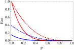
Figure 1: (color online) On the left $N_{A(BC)}$ (dashed) and $C_{A(BC)}^{2}$ (solid) for a state obtained when a phase damping channel acts locally and independently on each of the three qubits of an initial GHZ state (upper curves) and a generalized one, which without normalization is $0.2|000\rangle+|111\rangle$. On the right $C_{A(BC)}^{2}$ for a family of generalized GHZ states, $1|000\rangle+\beta|111\rangle$. For the two states used on the left and the ones on the right $C_{A(BC)}^{2}=N_{A(BC)}^{2}$.

The second possibility is to look at the action of the amplitude damping in a generalized W state. In this case $N_{A(BC)}^{2}\neq C_{A(BC)}^{2}$, but they have a qualitative similar behaviour. As an illustration, Fig. 2 shows both of them for the W state (upper curves in red) and a generalized one (lower curves in blue), which without normalization is $|001\rangle+5|010\rangle+10|100\rangle$. Note that the difference between the two measures increases with decoherence at the beginning and then goes to zero again. In fact if $N_{A(BC)}^{2}$ is equal to zero, then $C_{A(BC)}^{2}$ should also be, since there are no bound entangled states of rank 2 (Horodecki et al., 2003).

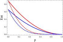
Figure 2: (color online) $C_{A(BC)}^{2}$ (solid) and $N_{A(BC)}^{2}$ (dashed) obtained when an amplitude damping channel acts locally and independently on each qubit of an initial W state (upper curves) and a generalized one, which without normalization is $|001\rangle+5|010\rangle+10|100\rangle$.

After viewing the difference between $C_{A(BC)}^{2}$ and $N_{A(BC)}^{2}$ I investigate the distribution of the bipartite entanglement, using the concurrence as the measure of entanglement between qubits. In Fig. 3 I show this distribution in terms of the concurrence for the W state (left) and a generalized one (right), which without normalization is $|001\rangle+2|010\rangle+3|100\rangle$. There the behavior of the entanglement between one qubit and the rest for differents focus, $C_{A(BC)}^{2}$, for example, under decoherence can be seen as solid curves. The entanglement between individual qubits is shown in dotted curves, while the residual entanglement is not show as it is null at the begginig and for any value of $p$. This indicates that the sum of the bipartite entanglement between the qubits decays at the same rate of the entanglement between one qubit and the rest. Fig. 4 is analogous but in terms of the negativity: we have $N_{AB}^{2}$ instead of $C_{AB}^{2}$. In this case the residual entanglement $\tau_{ABC}^{N}$ (dashed curve) may increase under the action of the local decoherence, indicating that this cannot be a good entanglement quantifier.

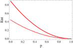
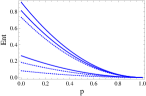
Figure 3: (color online) The distribution of entanglement in terms of the concurrence as a function of $p$, when an amplitude damping channel acts locally and independently on each qubit of an initial W state (left) and a generalized one (right), which without normalization is $|001\rangle+2|010\rangle+3|100\rangle$: $C_{A(BC)}^{2}$, $C_{B(AC)}^{2}$ and $C_{C(AB)}^{2}$ are ploted as solid lines from top to the bottom, respectively. $C_{AB}^{2}$, $C_{AC}^{2}$ and $C_{BC}^{2}$ are given by dotted lines from top to the bottom, respectively. The residual entanglement $\tau_{ABC}^{c}$, is null for any value of $p$.

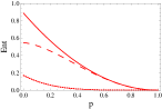
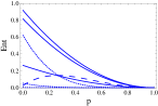
Figure 4: (color online) The distribution of entanglement in terms of the negativity as a function of $p$, when an amplitude damping channel acts locally and independently on each qubit of an initial W state (left) and a generalized one (right), which without normalization is $|001\rangle+2|010\rangle+3|100\rangle$: $C_{A(BC)}^{2}$, $C_{B(AC)}^{2}$ and $C_{C(AB)}^{2}$ are ploted as solid lines from top to the bottom, respectively. $N_{AB}^{2}$, $N_{AC}^{2}$ and $N_{BC}^{2}$ are given by dotted lines from top to the bottom, respectively. The residual entanglement $\tau_{ABC}^{N}$ is show in dashed. Note that it may increase, showing that it cannot be an entanglement monotone.

V Conclusions

In sum, I first investigated the behavior of the squared negativity and its pure state convex roof extension under some models of decoherence for the generalized GHZ and generalized W states. While they are equal for the generalized GHZ state, that is not true for the generalized W state. However in this last case they exhibit similar qualitative behavior decaying with the decoherence even tough their difference can increase.

I also studied how the distribution of entanglement behaves under these models of decoherence making use of the monogamy inequality for mixed states in terms of the concurrence and the negativity. For this aim I compared the behavior of the entanglement between one qubit and the other two treated as a single system with the one between individuals qubits. For the generalized W state I found out cases where the residual entanglement in terms of the negativity can increase under local decoherence even when all the bipartite entanglement is decaying, showing that it can not be a good entanglement measure.

In relation to the behaviour of multipartite entanglement under decoherence these results show no qualitative difference between the bipartite and multipartite entanglement for generalized GHZ and W states. However it would be interesting to be able to study these monogamy relations for states with richer entanglement structure than the GHZ and the W states. Would it be possible to happen that the bipartite entanglement between individuals qubits goes to zero while the multipartite one is still finite, and maybe only goes to zero asymptotically (sudden death of only bipartite entanglement)? We expect the rate of decay of both parts to be equal, since the tripartite entanglement should not increase under local operations. How about non-local environments?

These studies could also increase our understandig of multipartite entanglement per si. For know, we showed that the residual entanglement in terms of the negativity as used here can not be considered as a good entanglement measure. But, as mentioned before, one ca also define the residual entanglement for mixed states as the convex roof of the pure state residual entanglement (Lohmayer et al., 2006). And there are many other proposals of generalizations for higher Hilbert space dimensions and more than three particles ( (Wong and Christensen, 2001; shui Yu and shan Song, 2005, 2006; Cai et al., 2006; Ou et al., 2007; Ou, 2007; Bai et al., 2007; Adesso and Illuminati, 2007), for example). Therefore, it would be interesting to investigate the behavior of these others measures under decoherence.