Growth factor parametrization in curved space

Abstract

The growth rate of matter perturbation and the expansion rate of the Universe can be used to distinguish modified gravity and dark energy models in explaining cosmic acceleration. We explore here the inclusion of spatial curvature into the growth factor. We expand previous results using the approximation $\Omega_{m}^{\gamma}$ and then suggest a new form, $f_{a}=\Omega_{m}^{\gamma}+(\gamma-4/7)\Omega_{k}$, as an approximation for the growth factor when the curvature $\Omega_{k}$ is not negligible, and where the growth index $\gamma$ is usually model dependent. The expression recovers the standard results for the curved and flat $\Lambda$CDM and Dvali-Gabadadze-Porrati models. Using the best fit values of $\Omega_{m0}$ and $\Omega_{k0}$ to the expansion/distance measurements from Type Ia supernovae, baryon acoustic oscillation, WMAP5, and $H(z)$ data, we fit the growth index parameter to current growth factor data and obtain $\gamma_{\Lambda}\left(\Omega_{k}\not=0\right)=0.65^{+0.17}_{-0.15}$ and $\gamma_{DGP}\left(\Omega_{k}\not=0\right)=0.53^{+0.14}_{-0.12}$. For the $\Lambda$CDM model, the 1-$\sigma$ observational bounds are found consistent with theoretical value, unlike the case for the Dvali-Gabadadze-Porrati model. We also find that the current data we used is not enough to put significant constraints when the 3 parameters in $f_{a}$ are fit simultaneously. Importantly, we find that, in the presence of curvature, the analytical expression proposed for $f_{a}$ provides a better fit to the growth factor than other forms and should be useful for future high precision missions and studies.

I Introduction

The discovery of late time cosmic acceleration acc1 challenges our understanding of the standard models of gravity and particle physics. Within the framework of Friedmann-Robertson-Walker cosmology, a dark energy component with negative pressure is invoked to explain the observed accelerated expansion of the Universe. One simple candidate of dark energy which is consistent with current observations is the cosmological constant. By choosing a suitable equation of state $w=p/\rho$ for dark energy, we can recover the observed expansion rate $H(z)$ and the luminosity distance redshift relation $d_{L}(z)$. Many parametric and nonparametric model-independent methods were proposed to study the property of dark energy, see for example astier01 ; huterer ; par2 ; par3 ; lind ; alam ; jbp ; par4 ; par1 ; par5 ; gong04 ; gong05 ; gong06 ; gong08 ; Ishak2007 ; rev7 ; sahni and references therein.

The apparent acceleration of the Universe may be explained by the modification of gravitation, such as for example the Dvali-Gabadadze-Porrati (DGP) brane-world model dgp , in which gravity appears four dimensional at short distances but is modified at large distances. Recently, it was shown that the late cosmic acceleration of the Universe can also be realized in the Horava-Witten heterotic $M$ theory MTheory and string theory string on $S^{1}/Z_{2}$. It is remarkable that the acceleration is transient in all these models. To distinguish the effect of modified gravity from dark energy, we can use the growth rate of large scale in the Universe in addition to the distance data. While different models give the same late time accelerated expansion, the growth of matter perturbation they produce differs jetp . Recently, the use of the growth rate of matter perturbation in addition to the expansion history of the Universe to differentiate dark energy models and modified gravity attracted much attention, see, for example, an incomplete list huterer07 ; sereno ; knox ; ishak ; yun ; Aquavivaetal ; Danieletal ; polarski ; sapone ; balles ; gannouji ; berts ; laszlo ; kunz ; kiakotou ; porto ; wei ; ness and references therein. To the linear order of perturbation, at large scales, the matter density perturbation $\delta=\delta\rho_{m}/\rho_{m}$ satisfies the simple equation:

$$\ddot{\delta}+2H\dot{\delta}-4\pi G_{\rm eff}\,\rho_{m}\delta=0,$$ (1)

where $\rho_{m}$ is the matter energy density and $G_{\rm eff}$ denotes the effect of modified gravity. For example, $G_{\rm eff}/G=(4+2\omega)/(3+2\omega)$ for the Brans-Dicke theory boiss and $G_{\rm eff}/G=1+[3-6r_{c}H(1+\dot{H}/3H^{2})]^{-1}$ for the DGP model lue ; maartens , the dimensionless matter energy density $\Omega_{m}=8\pi G\rho_{m}/(3H^{2})$. In terms of the growth factor $f=d\ln\delta/d\ln a$, the matter density perturbation Eq. (1) becomes

$$f^{\prime}+f^{2}+\left(\frac{\dot{H}}{H^{2}}+2\right)f=\frac{3}{2}\frac{G_{eff}}{G}\Omega_{m},$$ (2)

where $f^{\prime}=df/d\ln a$. It is very interesting that the solution of the equation can be approximated as $f=\Omega_{m}^{\gamma}$ peebles ; fry ; lightman ; silveira ; wang ; gong08b and the growth index $\gamma$ can be obtained for some general models. The approximation was first proposed by Peebles for the matter dominated universe as $f(z=0)=\Omega^{0.6}_{0}$ peebles ; then a more accurate approximation, $f(z=0)=\Omega^{4/7}_{0}$, for the same model was derived in fry ; lightman . For a dynamical dark energy model with slowly varying $w$ and zero curvature, the approximation $f(z)=\Omega(z)^{\gamma}$ was given in silveira ; wang . For more general dynamical dark energy models in flat space, it was found that $\gamma=0.55+0.05[1+w(z=1)]$ with $w>-1$ and $\gamma=0.55+0.02[1+w(z=1)]$ with $w<-1$ linder05 ; linder07 . For the flat DGP model, $\gamma=11/16$ linder07 .

Fitting $f(z)=\Omega(z)^{\gamma}$ to several sets of the most recently observational data, lately one of us found that $\gamma=0.64^{+0.17}_{-0.15}$ for the $\Lambda$CDM model and $\gamma=0.55^{+0.14}_{-0.13}$ for the Dvali-Gabadadze-Porrati model gong08b . In this paper, we shall generalize such studies to the case where the space is not flat. In particular, in Sec. II we consider the dark energy model with constant $w$, while in Sec. III we discuss the DGP model. In Sec. IV, we apply the union compilation of type Ia supernovae (SNe) data union , the baryon acoustic oscillation (BAO) measurement from the Sloan Digital Sky Survey sdss6 , the shift parameter, the acoustic scale $l_{A}$ and the redshift $z_{*}$ of the last scattering surface measured from the Wilkinson Microwave Anisotropy Probe 5 yr data (WMAP5) wmap5 , and the Hubble parameter data $H(z)$ hz1 ; hz2 . We also use the growth factor data $f(z)$ porto ; ness ; guzzo ; colless ; tegmark ; ross ; angela ; mcdonald ; viel1 ; viel2 to find the constraint on the growth index $\gamma$. We also fit our simple analytical expression $f_{a}=\Omega_{m}^{\gamma}+(\gamma-4/7)\Omega_{k}$ to all the data sets by allowing the three parameters $\Omega_{m0}$, $\Omega_{k0}$ and $\gamma$ all to vary. We conclude the paper in Sec. V.

It should be noted that when the Universe is not flat, the approximation $f(z)=\Omega_{m}^{0.6}+\Omega_{\Lambda}/30$ was proposed in martel and $f(z=0)=\Omega^{0.6}_{m0}+\Omega_{\Lambda 0}(1+\Omega_{m0}/2)/70$ in lahav for the $\Lambda$CDM model. From these works one can see that the approximation for the growth factor may not be simply $\Omega_{m}^{\gamma}$ when the curvature is not zero, and that the growth index $\gamma$ can still be used as the signature of modified gravity and dark energy models.

II Dark Energy Models with Curvature

For the curved dark energy model with a constant equation of state $w$, we have

$$\frac{\dot{H}}{H^{2}}=\frac{1}{2}\Omega_{k}-\frac{3}{2}[1+w(1-\Omega_{m}-\Omega_{k})].$$ (3)

The energy conservation equation tells us that

$$\Omega_{m}^{\prime}=3w\Omega_{m}(1-\Omega_{m}-\Omega_{k})-\Omega_{m}\Omega_{k}.$$ (4)

Substituting Eqs. (3) and (4) into Eq. (2), we get

$$[3w\Omega_{m}(1-\Omega_{m}-\Omega_{k})-\Omega_{m}\Omega_{k}]\frac{df}{d\Omega_{m}}+f^{2}+\left[\frac{1}{2}+\frac{1}{2}\Omega_{k}-\frac{3}{2}w(1-\Omega_{m}-\Omega_{k})\right]f=\frac{3}{2}\Omega_{m}.$$ (5)

Plugging $f=\Omega_{m}^{\gamma}$ into Eq. (5), we get

$$[3w(1-\Omega_{m}-\Omega_{k})-\Omega_{k}]\Omega_{m}\ln\Omega_{m}\frac{d\gamma}{d\Omega_{m}}+\left(\gamma-\frac{1}{2}\right)[3w(1-\Omega_{m}-\Omega_{k})-\Omega_{k}]+\Omega_{m}^{\gamma}-\frac{3}{2}\Omega_{m}^{1-\gamma}+\frac{1}{2}=0.$$ (6)

At high redshift, both $1-\Omega_{m}$ and $\Omega_{k}$ are small quantities and they evolve differently. If we expand Eq. (6) around $\Omega_{m}=1$, then we also need to deal with $\Omega_{k}\sim\Omega_{m}\,a$. If $\Omega_{k}=0$, to the first order of $(1-\Omega_{m})$, we get wang ; Discrepancy

$$\gamma=\frac{3(1-w)}{5-6w}+\frac{3}{125}\frac{(1-w)(1-3w/2)}{(1-6w/5)^{2}(1-12w/5)}(1-\Omega_{m}).$$ (7)

If we take $\Omega_{k}$ as a constant, then to the lowest order, we get

$$(\gamma-1/2)(3w+1)\Omega_{k}=0,$$ (8)

so $\gamma=1/2$ which is not consistent with other results. Therefore, we cannot take $\Omega_{k}$ as a constant. If we think that $\Omega_{k}$ and $1-\Omega_{m}$ are independently small quantities, then to the first order of $1-\Omega_{m}$ and $\Omega_{k}$, we get

$$\gamma_{b}=\frac{3(w-1)(1-\Omega_{m})-(3w+1)\Omega_{k}}{(6w-5)(1-\Omega_{m})-2(3w+1)\Omega_{k}}.$$ (9)

If $\Omega_{k}=0$, Eq. (9) recovers the result given by Eq. (7) for the flat space. If there is no dark energy, $\Omega_{k}=1-\Omega_{m}$, then Eq. (9) tells us that $\gamma=4/7$ which is consistent with the results obtained in fry ; lightman . For the $\Lambda$CDM model, we get $\gamma=[6(1-\Omega_{m})-2\Omega_{k}]/[11(1-\Omega_{m})-4\Omega_{k}]$. Equation (9) is also consistent with Eq. (15) in Mortonsonetal giving a very similar expression when expanded in terms of $\Omega_{de}=1-\Omega_{m}-\Omega_{k}$ and $\Omega_{k}$. Although the result in Eq. (9) is consistent with other results, the expression for $\gamma$ is perhaps too complicated to be a constant; and we derive below a more practical expression for $\gamma$ to distinguish between different models. This means that the approximation $\Omega_{m}^{\gamma}$ needs to be modified so that we can get a simple number to distinguish different models. Let us recall the approximation used for the curved model with a cosmological constant. Martel used the approximation $f=\Omega_{m}^{0.6}+\Omega_{\Lambda}/30$ martel . In lahav , the approximation $f=\Omega_{m}^{0.6}+\Omega_{\Lambda}(1+\Omega_{m}/2)/70$ was used. Following these ideas, we propose the approximation $f_{a}=\Omega_{m}^{\gamma}+\beta\Omega_{k}$. Now $\Omega_{m}$ and $\Omega_{k}$ are independent variables, so

$$f_{a}^{\prime}=\beta\Omega_{k}+\left(\beta\frac{\Omega_{k}}{\Omega_{m}}+\gamma\Omega_{m}^{\gamma-1}\right)\Omega_{m}^{\prime}+(\Omega_{m}^{\gamma}+\Omega_{m}^{\gamma-1}\Omega_{m}^{\prime})\Omega_{k}\ln\Omega_{m}\frac{\partial\gamma}{\partial\Omega_{k}}+\Omega_{m}^{\gamma}\Omega_{m}^{\prime}\ln\Omega_{m}\frac{\partial\gamma}{\partial\Omega_{m}}$$ (10)

Substituting the expression of $f_{a}$, Eqs. (4) and (10) into Eq. (2), expanding all quantities around $\Omega_{m}=1$ and $\Omega_{k}=0$, and then keeping terms linear in $1-\Omega_{m}-\Omega_{k}$ and $\Omega_{k}$, we finally find that

$$\gamma=\frac{3(1-w)}{5-6w},\quad\beta=\gamma-\frac{4}{7}.$$ (11)

Therefore, the approximation becomes

$$f_{a}=\Omega_{m}^{\gamma}+(\gamma-4/7)\Omega_{k},\quad\gamma=\frac{3(1-w)}{5-6w}.$$ (12)

For this approximation, we have only one constant $\gamma$ and this growth index can be used as the fingerprint of the model. When $\Omega_{k}=0$, the approximation (12) recovers the familiar result. For the $\Lambda$CDM model, the approximation is $f_{a}=\Omega_{m}^{6/11}-2\Omega_{k}/77$. This result is consistent with Eq. (15) in Mortonsonetal for $\gamma$ when the latter is used into their function $f(a)=\Omega_{m}(a)^{\gamma}$ and expanded around $\Omega_{k}=0$.

In order to see how well the approximation $f_{a}$ fits the growth factor $f$, we need to solve Eq. (2) numerically with the expression of $\Omega_{m}$ and $\Omega_{k}$. The dimensionless matter density is

$$\Omega_{m}=\frac{\Omega_{m0}}{\Omega_{m0}+\Omega_{k0}(1+z)^{-1}+(1-\Omega_{m0}-\Omega_{k0})(1+z)^{3w}},$$ (13)

and the dimensionless curvature density is

$$\Omega_{k}=\frac{\Omega_{k0}(1+z)^{-1}}{\Omega_{m0}+\Omega_{k0}(1+z)^{-1}+(1-\Omega_{m0}-\Omega_{k0})(1+z)^{3w}}.$$ (14)

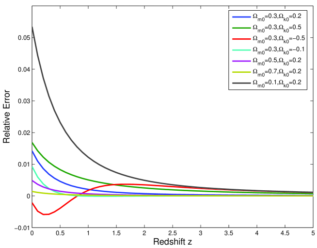
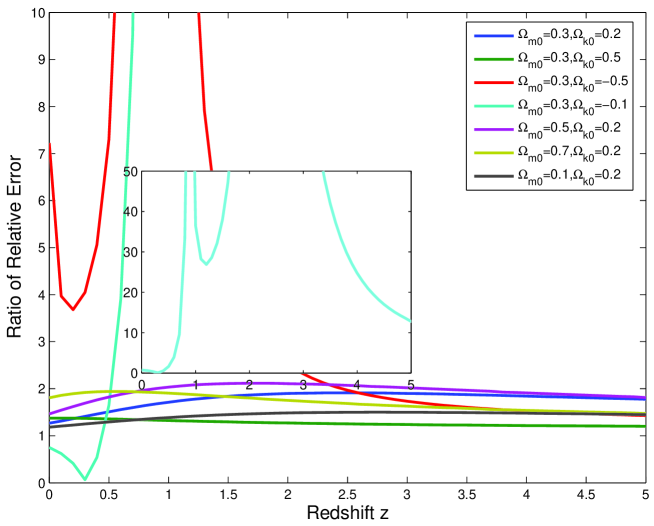
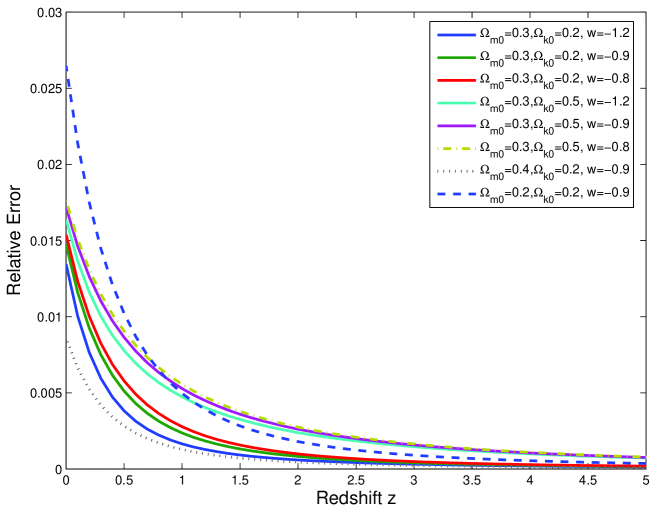
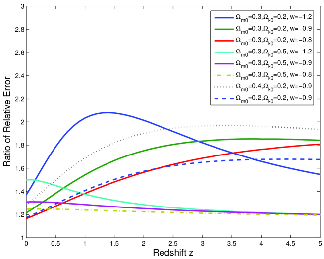
By using the above Eqs. (13) and (14), we solve Eq. (2) numerically to get the growth factor $f$ for different values of $\Omega_{m0}$, $\Omega_{k0}$ and $w$. Then we compare the approximation $f_{a}$ with $f$ by plotting the relative error $(f_{a}-f)/f$ for the $\Lambda$CDM model in Fig. 1. From there we see that the error of the approximation is a few percent, so $f_{a}$ approximates $f$ very well. We also compare the approximation $\Omega_{m}^{\gamma_{b}}$ with $\gamma_{b}$ given by Eq. (9) with the approximation $f_{a}$ by plotting the absolute value of the ratio $|(\Omega_{m}^{\gamma_{b}}-f)/(f_{a}-f)|$ in Fig.2, from which we see that $f_{a}$ approximates $f$ better. For the dark energy model with constant $w$, the accuracy of the approximation $f_{a}$ is shown in Fig. 3 and the comparison between the approximation of $f_{a}$ and $f_{b}$ is shown in Fig. 4 for some typical values of $\Omega_{m0}$, $\Omega_{k0}$ and $w$. The approximation $f_{a}$ is not only a better approximation, but also has a simpler expression for the growth index $\gamma$. Therefore, we should use Eq. (12) to approximate the growth factor.

Figure 1: The relative difference between the growth factor $f$ and the approximation $f_{a}$ with $\gamma=6/11$ in Eq. (12) for the $\Lambda$CDM model.

Figure 2: The ratio $|(\Omega_{m}^{\gamma_{b}}-f)/(f_{a}-f)|$ of the two different approximations of the growth factor for the $\Lambda$CDM model. Since the case with $\Omega_{m0}=0.3$ and $\Omega_{k0}=-0.1$ was cut off in the plot, we show it explicitly in the inset.

Figure 3: The relative difference between the growth factor $f$ and the approximation $f_{a}$ in Eq. (12) for the dark energy model with constant $w$.

Figure 4: The ratio $|(f_{a}-f)/(\Omega_{m}^{\gamma_{b}}-f)|$ of the two different approximations of the growth factor for the dark energy model with constant $w$.

III DGP models with curvature

For the DGP model, we have

$$\frac{G_{\rm eff}}{G}=\frac{4\Omega_{m}^{2}-4(1-\Omega_{k})^{2}+2\sqrt{1-\Omega_{k}}(3-4\Omega_{k}+2\Omega_{m}\Omega_{k}+\Omega_{k}^{2})}{3\Omega_{m}^{2}-3(1-\Omega_{k})^{2}+2\sqrt{1-\Omega_{k}}(3-4\Omega_{k}+2\Omega_{m}\Omega_{k}+\Omega_{k}^{2})}.$$ (15)

The Friedmann equation gives

$$\frac{\dot{H}}{H^{2}}=-\Omega_{k}-\frac{3\Omega_{m}(1-\Omega_{k})}{1+\Omega_{m}-\Omega_{k}}.$$ (16)

The energy conservation equation tells us that

$$\Omega_{m}^{\prime}=-\Omega_{m}\left(3-2\Omega_{k}-\frac{6\Omega_{m}(1-\Omega_{k})}{1+\Omega_{m}-\Omega_{k}}\right).$$ (17)

As discussed in the previous section, we consider the approximation $f_{a}=\Omega_{m}^{\gamma}+\beta\Omega_{k}$. Substituting the expression of $f_{a}$, Eqs. (17) and (10) into Eq. (2), expanding all quantities around $\Omega_{m}=1$ and $\Omega_{k}=0$, and then keeping terms linear in $1-\Omega_{m}-\Omega_{k}$ and $\Omega_{k}$, we obtain

$$\left[2+\frac{7}{2}(\beta-\gamma)\right]\Omega_{k}+\left[-4\gamma+\frac{11}{4}\right](1-\Omega_{m}-\Omega_{k})=0.$$ (18)

Therefore, the approximation of the growth factor for the DGP model is

$$f_{a}=\Omega_{m}^{11/16}+\left(\frac{11}{16}-\frac{4}{7}\right)\Omega_{k}.$$ (19)

On the other hand, if we approximate the growth factor $f$ by $\Omega_{m}^{\gamma_{b}}$, then set $\beta=0$ in Eq. (18), finally we find

$$\gamma_{b}=\frac{11(1-\Omega_{m})-3\Omega_{k}}{16(1-\Omega_{m})-2\Omega_{k}}.$$ (20)

In the DGP model, the dimensionless matter energy density is given by

$$\Omega_{m}=\frac{\Omega_{m0}(1+z)^{3}}{\Omega_{k0}(1+z)^{2}+[\Omega_{r0}+\sqrt{\Omega_{m0}(1+z)^{3}+\Omega_{r0}^{2}}\,]^{2}},$$ (21)

where $\Omega_{r0}=(1-\Omega_{m0}-\Omega_{k0})/2\sqrt{1-\Omega_{k0}}$. The dimensionless curvature energy density is

$$\Omega_{k}=\frac{\Omega_{k0}(1+z)^{2}}{\Omega_{k0}(1+z)^{2}+[\Omega_{r0}+\sqrt{\Omega_{m0}(1+z)^{3}+\Omega_{r0}^{2}}\,]^{2}}.$$ (22)

Combining Eqs. (2), (15), (16), (21) and (22), we get the evolution of the growth factor $f$, and the result is then compared with the approximation $f_{a}$. In Fig. 5, we show the accuracy of the approximation by plotting $(f_{a}-f)/f$.

Figure 5: The relative difference between the growth factor $f$ and $f_{a}$ with $\gamma=11/16$ for the DGP model.

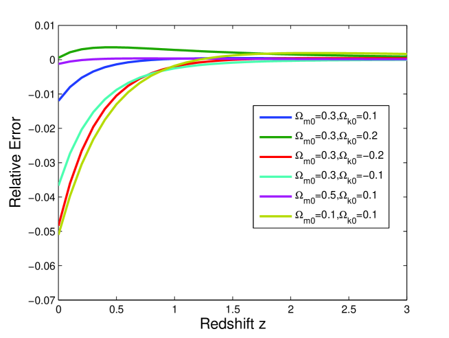
From Fig. 5, we see that the error is under 10%. We also checked the accuracy of the approximation $\Omega_{m}^{\gamma_{b}}$ and find that the approximation $f_{a}$ is usually better for the model we are interested in.

IV Observational Constraints

Now we use the observational data to fit the dark energy model with constant $w$ and the DGP model. The parameters in the models are determined by minimizing $\chi^{2}=\chi^{2}_{sn}+\chi^{2}_{bao}+\chi^{2}_{cmb}+\chi^{2}_{h}$. For the Type Ia SNe data, we use the reduced union compilation of 307 Type Ia SNe union . The union compilation has 57 nearby Type Ia SNe and 250 high-$z$ Type Ia SNe. It includes the Supernova Legacy Survey astier and the ESSENCE Survey riess ; essence , the older observed SNe data, and the extended data set of distant SNe observed with the Hubble space telescope. To fit the Type Ia SNe data, we define

$$\chi^{2}_{sn}=\sum_{i=1}^{307}\frac{[\mu_{obs}(z_{i})-\mu(z_{i})]^{2}}{\sigma^{2}_{i}},$$ (23)

where the extinction-corrected distance modulus $\mu(z)=5\log_{10}[d_{L}(z)/{\rm Mpc}]+25$, $\mu_{obs}$ is the observed distance modulus, $\sigma_{i}$ is the total uncertainty in the SNe data, and the luminosity distance is

$$d_{L}(z)=\frac{1+z}{H_{0}\sqrt{|\Omega_{k}|}}{\rm sinn}\left[\sqrt{|\Omega_{k}|}\int_{0}^{z}\frac{dz^{\prime}}{E(z^{\prime})}\right],$$ (24)

where

$${\rm sinn}(\sqrt{|\Omega_{k}|}x)=\begin{cases}\sin(\sqrt{|\Omega_{k}|}x),&{\rm if}\ \Omega_{k}<0,\\ \sqrt{|\Omega_{k}|}x,&{\rm if}\ \Omega_{k}=0,\\ \sinh(\sqrt{|\Omega_{k}|}x)&{\rm if}\ \Omega_{k}>0,\end{cases}$$ (25)

and the dimensionless Hubble parameter $E(z)=H(z)/H_{0}=[\Omega_{0}(1+z)^{3}+(1-\Omega_{0})(1+z)^{3(1+w)}]^{1/2}$ for the dark energy model with constant $w$ and $E(z)=[\Omega_{0}(1+z)^{3}+(1-\Omega_{0})^{2}/4]^{1/2}+(1-\Omega_{0})/2$ for the DGP model.

To use the BAO measurement from the Sloan Digital Sky Survey data, we define sdss6

$$\chi^{2}_{bao}=\left(\frac{r_{z}(z_{d})/D_{V}(z=0.2)-0.198}{0.0058}\right)^{2}+\left(\frac{r_{z}(z_{d})/D_{V}(z=0.35)-0.1094}{0.0033}\right)^{2},$$ (26)

where the effective distance is

$$D_{V}(z)=\left[\frac{d_{L}^{2}(z)}{(1+z)^{2}}\frac{z}{H(z)}\right]^{1/3}.$$ (27)

The redshift $z_{d}$ is fitted with the formulas hu98

$$z_{d}=\frac{1291(\Omega_{m}h^{2})^{0.251}}{1+0.659(\Omega_{m}h^{2})^{0.828}}[1+b_{1}(\Omega_{b}h^{2})^{b_{2}}],$$ (28)

$$b_{1}=0.313(\Omega_{m}h^{2})^{-0.419}[1+0.607(\Omega_{m}h^{2})^{0.674}],\quad b_{2}=0.238(\Omega_{m}h^{2})^{0.223},$$ (29)

and the comoving sound horizon is

$$r_{s}(z)=\int_{0}^{\infty}\frac{dz^{\prime}}{c_{s}(z^{\prime})E(z^{\prime})},$$ (30)

where the sound speed $c_{s}(z)=1/\sqrt{3[1+\bar{R_{b}}/(1+z)}]$, $\bar{R_{b}}=315000\Omega_{b}h^{2}(T_{cmb}/2.7{\rm K})^{-4}$.

To implement the WMAP5 data, we need to add three fitting parameters $R$, $l_{a}$ and $z_{*}$, so $\chi^{2}_{cmb}=\Delta x_{i}{\rm Cov}^{-1}(x_{i},x_{j})\Delta x_{j}$, where $x_{i}=(R,\ l_{a},\ z_{*})$ denotes the three parameters for the WMAP5 data, $\Delta x_{i}=x_{i}-x_{i}^{obs}$ and Cov$(x_{i},x_{j})$ is the covariance matrix for the three parameters wmap5 . The acoustic scale $l_{A}$ is

$$l_{A}=\frac{\pi d_{L}(z_{*})}{(1+z_{*})r_{s}(z_{*})},$$ (31)

where the redshift $z_{*}$ is given by hu96

$$z_{*}=1048[1+0.00124(\Omega_{b}h^{2})^{-0.738}][1+g_{1}(\Omega_{m}h^{2})^{g_{2}}]=1090.04\pm 0.93,$$ (32)

$$g_{1}=\frac{0.0783(\Omega_{b}h^{2})^{-0.238}}{1+39.5(\Omega_{b}h^{2})^{0.763}},\quad g_{2}=\frac{0.560}{1+21.1(\Omega_{b}h^{2})^{1.81}}.$$ (33)

The shift parameter

$$R=\frac{\sqrt{\Omega_{m}}}{\sqrt{|\Omega_{k}|}}{\rm sinn}\left(\sqrt{|\Omega_{k}|}\int_{0}^{z_{*}}\frac{dz}{E(z)}\right)=1.710\pm 0.019.$$ (34)

Simon, Verde, and Jimenez obtained the Hubble parameter $H(z)$ at nine different redshifts from the differential ages of passively evolving galaxies hz1 . Recently, the authors in hz2 obtained $H(z=0.24)=83.2\pm 2.1$ and $H(z=0.43)=90.3\pm 2.5$ by taking the BAO scale as a standard ruler in the radial direction. To use these 11 $H(z)$ data, we define

$$\chi^{2}_{h}=\sum_{i=1}^{11}\frac{[H_{obs}(z_{i})-H(z_{i})]^{2}}{\sigma_{hi}^{2}},$$ (35)

where $\sigma_{hi}$ is the $1\sigma$ uncertainty in the $H(z)$ data. We also add the prior $H_{0}=72\pm 8$ km/s/Mpc given by Freedman et al. freedman . The likelihood for the parameters in the model and the nuisance parameters $\Omega_{b}h^{2}$ and $H_{0}$ is computed using a Monte Carlo Markov Chain (MCMC). The MCMC method randomly chooses values for the above parameters, evaluates $\chi^{2}$, and determines whether to accept or reject the set of parameters using the Metropolis-Hastings algorithm. The set of parameters that is accepted to the chain forms a new starting point for the next process, and the process is repeated for a sufficient number of steps until the required convergence is reached. Our MCMC code is based on the publicly available package COSMOMC cosmomc .

Figure 6: The $1\sigma$ and $2\sigma$ contours of $\Omega$ and $w$ by fitting the dark energy model with constant $w$ to the combined data. The point with $+$ denotes the flat $\Lambda$CDM point $\Omega_{k}=0$ and $w=-1$.

Figure 7: The $1\sigma$ and $2\sigma$ contours of $\Omega_{m}$ and $\Omega_{k}$ for the $\Lambda$CDM model.

Figure 8: The $1\sigma$ and $2\sigma$ contours of $\Omega_{m}$ and $\Omega_{k}$ for the DGP model.

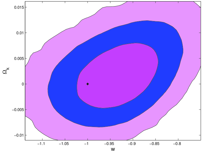
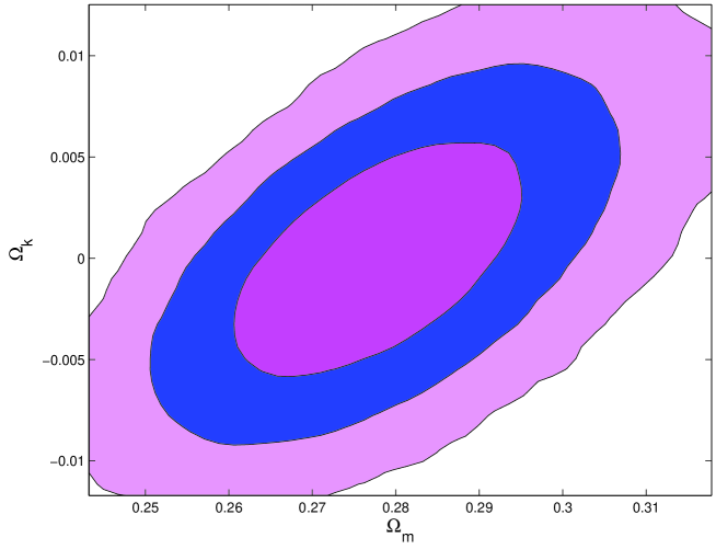
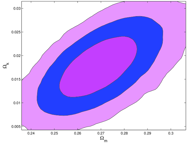
By fitting the dark energy model with constant $w$ to the combined data (except the growth data that we use next), we get $\chi^{2}=332.6$, $\Omega_{m0}=0.276^{+0.028}_{-0.026}$, $\Omega_{k0}=0.002\pm 0.010$ and $w=-0.93^{+0.14}_{-0.15}$. The $1\sigma$, $2\sigma$ and $3\sigma$ contours of $\Omega_{k0}$ and $w$ are shown in Fig. 6. By fitting the $\Lambda$CDM model to the combined data, we get $\chi^{2}=333.9$, $\Omega_{m0}=0.277^{+0.025}_{-0.023}$ and $\Omega_{k0}=0.0002\pm 0.0081$. The $1\sigma$, $2\sigma$ and $3\sigma$ contours of $\Omega_{m0}$ and $\Omega_{k0}$ are shown in Fig. 7. By fitting the DGP model to the combined data, we get $\chi^{2}=345.7$, $\Omega_{m0}=0.268^{+0.024}_{-0.022}$ and $\Omega_{k0}=0.018\pm 0.009$. The $1\sigma$, $2\sigma$ and $3\sigma$ contours of $\Omega_{k0}$ and $w$ are shown in Fig. 8.

Next, if we use constraints on $\Omega_{m0}$ and $\Omega_{k0}$ from previous step and fit $\Omega_{m}^{\gamma}+(\gamma-4/7)\Omega_{k}$ to the growth factor data $f(z)$ alone from porto ; ness ; guzzo ; colless ; tegmark ; ross ; angela ; mcdonald ; viel1 ; viel2 , we can get a constraint on the growth index $\gamma$. For the curved $\Lambda$CDM model with the best fit value $\Omega_{m0}=0.277$ and $\Omega_{k0}=0.0002$, we find that $\chi^{2}=4.54$ and $\gamma_{\Lambda}=0.65^{+0.17}_{-0.15}$. The theoretical value $\gamma_{\infty}=6/11=0.55$ is consistent with the observation at the $1\sigma$ level. For the DGP model with the best fit value $\Omega_{m0}=0.268$ and $\Omega_{k0}=0.018$, we find $\chi^{2}=5.79$ and $\gamma_{DGP}=0.53^{+0.14}_{-0.12}$ which is not consistent with the theoretical value $\gamma_{\infty}=11/16=0.6875$ at the $1\sigma$ level.

We also fit $\Omega_{m}^{\gamma}+(\gamma-4/7)\Omega_{k}$ to the combined Type Ia, the BAO, the CMB, the Hubble parameter $H(z)$, and the growth factor $f(z)$ data, and allowing for the three parameters to vary. We obtain the following constraints on the parameters $\Omega_{m0}$, $\Omega_{k0}$ and $\gamma$. For the curved $\Lambda$CDM model, we find that $\chi^{2}=338.4$, $\Omega_{m0}=0.276^{+0.03}_{-0.024}(1\sigma)^{+0.041}_{-0.033}(2\sigma)$, $\Omega_{k0}=-0.0002^{+0.0095}_{-0.0086}(1\sigma)^{+0.0132}_{-0.0118}(2\sigma)$, and $\gamma=0.64^{+0.48}_{-0.32}(1\sigma)^{+0.73}_{-0.43}(2\sigma)$. For the DGP model, we find that $\chi^{2}=351.47$, $\Omega_{m0}=0.268^{+0.028}_{-0.024}(1\sigma)^{+0.039}_{-0.033}(2\sigma)$, $\Omega_{k0}=0.017^{+0.011}_{-0.009}(1\sigma)^{+0.015}_{-0.013}(2\sigma)$, and $\gamma=0.52^{+0.40}_{-0.27}(1\sigma)^{+0.61}_{-0.35}(2\sigma)$. Proceeding in this second way shows that current data that we used is not enough in order to put conclusive constraints on $\gamma$ and the underlying theory of gravity; however, this is likely to change with future data from future high precision missions such as PLANCK, JDEM, LSST, and others.

V Discussions

We find that the simple analytical expression $f_{a}=\Omega_{m}^{\gamma}+(\gamma-4/7)\Omega_{k}$ can be used to approximate very well the growth factor $f$ when the curvature is not zero and this is the main result of the paper. The curvature parameter is included, as shown above, into the function $f_{a}$ which is found to provide a better fit to the growth factor than $\Omega_{m}^{\gamma}$ (with curvature included in $\gamma$) when compared to the growth factor evaluated numerically from the differential equation (this is shown in Figs 3-5). We also find that, with $f_{a}$ as given above, the asymptotic value of $\gamma$ is the same as that in flat space and it provides distinctive information about a dark energy model versus a modification of gravity. For example, $\gamma\approx 0.55$ for the $\Lambda$CDM model and $\gamma=0.6875$ for the DGP model.

We explored then some constraints on $\gamma$ using the form of $f_{a}$ above and current data from Type Ia SNe, BAO, WMAP5, $H(z)$ data, and growth factor data. Unlike previous analyses which used the shift parameter for the WMAP5 data and the $A$ parameter for the BAO data gong08b , here we used the shift parameter $R$, the acoustic scale $l_{A}$, the redshift $z_{*}$ and their covariance matrix for the WMAP5 data wmap5 , and the parameter $r_{s}(z_{d})/D_{V}(z)$ at two different redshifts for the BAO data.

First, we fit the models to the combined Type Ia SNe, BAO, WMAP5, and $H(z)$ data and obtained $\Omega_{m0}=0.277^{+0.025}_{-0.023}$, $\Omega_{k0}=0.0002\pm 0.0081$ and $\chi^{2}=333.9$ for the curved $\Lambda$CDM model, and $\Omega_{m0}=0.268^{+0.024}_{-0.022}$, $\Omega_{k0}=0.018\pm 0.009$ and $\chi^{2}=345.7$ for the DGP model. The DGP model is found strongly disfavored by the data, a result consistent with other analysis song ; song05 ; roy06 ; gong ; zhu ; gong08b . Comparing with the WMAP5 result wmap5 , we see that the error bar becomes a little bigger with the addition of the $H(z)$ data. The reason is due to the larger uncertainties in the $H(z)$ data. Now, using the best fit values for $\Omega_{m0}$ and $\Omega_{k0}$ from the previous step and the growth data of $f(z)$, we obtained constraints on the growth index $\gamma$. For the curved $\Lambda$CDM model, we find that $\gamma_{\Lambda}=0.65^{+0.17}_{-0.15}$, which is consistent with the theoretical value 0.55. This result is also consistent with those in ness ; porto ; gong08b . For the DGP model, we find that $\gamma_{DGP}=0.53^{+0.14}_{-0.12}$. The theoretical value $\gamma=0.6875$ lies outside the $1\sigma$ bounds thus again disfavoring the DGP model.

Next, we fit $f_{a}$ to all the data sets by allowing the three parameters $\Omega_{m0}$, $\Omega_{k0}$ and $\gamma$ to vary. For the curved $\Lambda$CDM model, we find that $\chi^{2}=338.4$, $\Omega_{m0}=0.276^{+0.03}_{-0.024}(1\sigma)^{+0.041}_{-0.033}(2\sigma)$, $\Omega_{k0}=-0.0002^{+0.0095}_{-0.0086}(1\sigma)^{+0.0132}_{-0.0118}(2\sigma)$, and $\gamma=0.64^{+0.48}_{-0.32}(1\sigma)^{+0.73}_{-0.43}(2\sigma)$. For the curved DGP model, we find that $\chi^{2}=351.47$, $\Omega_{m0}=0.268^{+0.028}_{-0.024}(1\sigma)^{+0.039}_{-0.033}(2\sigma)$, $\Omega_{k0}=0.017^{+0.011}_{-0.009}(1\sigma)^{+0.015}_{-0.013}(2\sigma)$, and $\gamma=0.52^{+0.40}_{-0.27}(1\sigma)^{+0.61}_{-0.35}(2\sigma)$. Thus, the current data is still not sufficient for us to obtain conclusive constraints, when we fit all these three parameters simultaneously. But this is likely to be improved substantially with future high precision missions.

Finally, the inclusion of the curvature in future analyses of cosmological data in order to constrain the origin of cosmic acceleration was recently discussed and stressed in the literature, e.g. wmap5 ; virey ; gong08 . This includes the question of distinguishing dark energy from modified gravity using the growth data in the presence of spatial curvature. We find here that the analytical expression $f_{a}=\Omega_{m}^{\gamma}+(\gamma-4/7)\Omega_{k}$ approximates very well the growth factor $f$ when curvature is added and should be useful for such future analyses.