Pseudo–magnetorotational instability in a Taylor-Dean flow between electrically connected cylinders

Abstract

We consider a Taylor-Dean-type flow of an electrically conducting liquid in an annulus between two infinitely long perfectly conducting cylinders subject to a generally helical magnetic field. The cylinders are electrically connected through a remote, perfectly conducting endcap, which allows a radial electric current to pass through the liquid. The radial current interacting with the axial component of magnetic field gives rise to the azimuthal electromagnetic force, which destabilizes the base flow by making its angular momentum decrease radially outwards. This instability, which we refer to as the pseudo–magnetorotational instability (MRI), looks like an MRI although its mechanism is basically centrifugal. In a helical magnetic field, the radial current interacting with the azimuthal component of the field gives rise to an axial electromagnetic force, which drives a longitudinal circulation. First, this circulation advects the Taylor vortices generated by the centrifugal instability, which results in a traveling wave as in the helical MRI (HMRI). However, the direction of travel of this wave is opposite to that of the true HMRI. Second, at sufficiently strong differential rotation, the longitudinal flow becomes hydrodynamically unstable itself. For electrically connected cylinders in a helical magnetic field, hydrodynamic instability is possible at any sufficiently strong differential rotation. In this case, there is no hydrodynamic stability limit defined in the terms of the critical ratio of rotation rates of inner and outer cylinders that would allow one to distinguish a hydrodynamic instability from the HMRI. These effects can critically interfere with experimental as well as numerical determination of MRI.

I Introduction

The magnetorotational instability (MRI) can account for the formation of stars and entire galaxies in the accretion disks. For an object to form, the matter circling around it has to slow down by transferring its angular momentum outwards. The observed accretion rates suggest the angular momentum transfer in the astrophysical disks to be turbulent while the velocity distribution in them seems to be hydrodynamically stable. A possible solution to this problem was suggested by Balbus and Hawley Balbus-Hawley-1991 ; Balbus-Hawley-1998 , who pointed out that a Keplerian velocity distribution in accretion disk can be destabilized by a magnetic field in the process known as the MRI Velikhov-1959 ; Chandrasekhar-1960 . This proposition has triggered a number of experimental studies trying to reproduce MRI in laboratory Sisan-etal ; Nature-2006 . The main technical difficulty to such experiments is the magnetic Reynolds number Rm that is required to be $\sim 10$ at least. For a typical liquid metal with the magnetic Prandtl number $\textrm{Pm}\sim 10^{-5}-10^{-6},$ this corresponds to a hydrodynamic Reynolds number $\textrm{Re}=\textrm{Rm}/\textrm{Pm}\sim 10^{6}-10^{7}$ Goodman-Ji-2002 . Thus, the base flow on which the MRI is to be observed may be turbulent at such Reynolds numbers independently of MRI as in the experiment of Sisan et al. Sisan-etal . A possible solution to this problem was proposed by Hollerbach and Rüdiger Hollerbach-Ruediger-2005 , who suggested that MRI can take place in the Taylor-Couette (TC) flow at $\textrm{Re}\sim 10^{3}$ when the imposed magnetic field is helical rather than purely axial as in the classical case. Theoretical prediction of this new type of helical MRI (HMRI) was soon succeeded by a claim of its experimental observation by Stefani et al. Rued-apjl ; Stefani-etal ; Stefani-NJP . Subsequently, these experimental observations have been questioned by Liu et al. Liu-etal2006 who find no such instability in their inviscid theoretical analysis of finite length cylinders with insulating endcaps. In a more realistic numerical simulation, Liu et al. Liu-etal2007 confirm the experimental results, though note that there is no MRI at the experimental parameters when ideal TC boundary conditions are used. Szklarski Szklarski showed later that the ideal TC requires a slightly different parameters for the HMRI to set in. Despite the numerical evidence, Liu et al. Liu-etal2007 ; Liu2008 suspected the observed phenomenon to be a transient growth rather than a self-sustained instability. This paper shows that the observation of a self-sustained instability which looks like an MRI does not necessarily mean that the latter is MRI.

Recently, we found that HMRI can be self-sustained and thus experimentally observable in a system of sufficiently large axial extension because there is not only convective but also absolute HMRI threshold Priede-Gerbeth2008 . However, the comparison with the experimental results Rued-apjl ; Stefani-etal ; Stefani-NJP revealed that HMRI has been observed slightly beyond the range of its absolute instability, where it is expected to be self-sustained according to the ideal TC flow model. This discrepancy with the experimental observations is probably due to the deviation of the real base flow from the ideal TC flow used in the theoretical analysis. Such a deviation, however, poses a major problem for the interpretation of experimental results, especially for the identification of HMRI. Namely, the Rayleigh line defining the hydrodynamic stability limit of the ideal TC flow is used as a reference point to discriminate between a magnetically modified Taylor vortex flow and HMRI. The latter two are hardly distinguishable by the oscillation frequency, which varies weakly as the Rayleigh line is crossed. The main problem is the hydrodynamic stability limit of the real base flow, i.e., its actual Rayleigh line, which may differ from that of the ideal TC flow. Therefore the latter cannot be used for the interpretation of experimental results. This ambiguity is not resolved by the direct numerical simulation of the problem either even if there is a perfect agreement with the experiment. It is because the notion of MRI is based on the ideal TC flow with a fixed hydrodynamic stability limit, which is affected neither by the end effects nor by the magnetic field. Unfortunately, this is the case neither for experiments nor for numerical simulations. First, there is an Ekman pumping at the endcaps, which can spread up to significant but nevertheless limited distances into the base flow provided that the latter is hydrodynamically stable. The Ekman circulation can be reduced by using several independently rotating rings for the endcaps Nature-2006 or by splitting the latter into two rings of a certain size attached to the inner and outer cylinders, respectively Szklarski . Another important effect pointed out by Szklarski and Rüdiger Szklarski-Ruediger2007 , which can significantly affect the base flow, is related with the Hartmann layers forming at the endcaps in axial magnetic field.

In this paper, we show that there may be additional effects in the presence of a magnetic field when well conducting inner and outer cylinders are electrically connected through an endcap as in the original PROMISE experiment Rued-apjl ; Stefani-etal ; Stefani-NJP . The endcap acting in parallel with the Hartmann layer allows a radial current to close through the liquid between the cylinders. The interaction of radial current with axial magnetic field gives rise to an azimuthal electromagnetic force, which reduces the velocity difference between the endcap and the liquid above it. Depending on the strength of the magnetic field, this electromagnetic force can render the profile of azimuthal base flow centrifugally unstable. As a result, in axial magnetic field, the instability can extend significantly beyond the Rayleigh line similarly to the classical MRI. Moreover, in helical magnetic field, the interaction of radial current with the azimuthal component of magnetic field gives rise to an axial electromagnetic force, which drives a longitudinal flow. First, this longitudinal flow going upwards along the inner cylinder, where the azimuthal base flow is centrifugally destabilized, advects Taylor vortices that results in a traveling wave as in the HMRI. However, the direction in which these Taylor vortices are advected is opposite to the direction of travel of true HMRI wave. Second, for sufficiently large differential rotation, longitudinal flow may become linearly unstable at any rotation rate ratio.

The paper is organized as follows. In Sec. II we formulate the problem in the inductionless approximation. The base flow for electrically connected cylinders is derived in Sec. III. Section IV introduces the linear stability problem. Numerical results for axial and helical magnetic fields are presented in Secs. V.1 and V.2, respectively. The paper is concluded with a summary in Sec. VI.

II Problem formulation

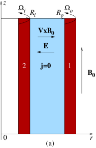
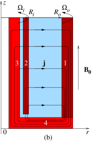
Figure 1: (a) An ideal electrically uncoupled system and (b) a real system with the inner and outer cylinders electrically connected via the endcap and inner vessel wall; (1) outer cylinder, (2) inner cylinder, (3) inner wall, (4) endcap.

Consider an incompressible fluid of kinematic viscosity $\nu$ and electrical conductivity $\sigma$ filling the annulus between two long, concentric cylinders with inner radius $R_{i}$ and outer radius $R_{o}$ rotating with angular velocities $\Omega_{i}$ and $\Omega_{o}.$ The flow is subject to a generally helical, steady external magnetic field $\mbox{\boldmath$\mathrm{B}$}_{0}=B_{\phi}\mbox{\boldmath$\mathrm{e}$}_{\phi}+B_{z}\mbox{\boldmath$\mathrm{e}$}_{z}$ with axial and azimuthal components $B_{z}=B_{0}$ and $B_{\phi}=\beta B_{0}R_{i}/r$ in cylindrical coordinates $(r,\phi,z),$ where $\beta$ is a dimensionless parameter characterizing the geometrical helicity of the field. The fluid is supposed to be poorly conducting so that the induced magnetic field is negligible with respect to the imposed one. This corresponds to the so-called inductionless approximation, which holds for the HMRI characterized by small magnetic Reynolds number $\textrm{Rm}=\mu_{0}\sigma v_{0}L\ll 1,$ where $\mu_{0}$ is the permeability of vacuum, $v_{0}$ and $L$ are the characteristic velocity and length scale Priede-etal-2007 . The velocity of fluid flow $\mathrm{v}$ is governed by the Navier-Stokes equation with electromagnetic body force

$$\frac{\partial\mbox{\boldmath$\mathrm{v}$}}{\partial t}+(\mbox{\boldmath$\mathrm{v}$}\cdot\mbox{\boldmath$\mathrm{\nabla}$})\mbox{\boldmath$\mathrm{v}$}=-\frac{1}{\rho}\mbox{\boldmath$\mathrm{\nabla}$}p+\nu\mbox{\boldmath$\mathrm{\nabla}$}^{2}\mbox{\boldmath$\mathrm{v}$}+\frac{1}{\rho}\mbox{\boldmath$\mathrm{j}$}\times\mbox{\boldmath$\mathrm{B}$}_{0},$$ (1)

where the induced current follows from Ohm’s law for a moving medium

$$\mbox{\boldmath$\mathrm{j}$}=\sigma\left(\mbox{\boldmath$\mathrm{E}$}+\mbox{\boldmath$\mathrm{v}$}\times\mbox{\boldmath$\mathrm{B}$}_{0}\right).$$ (2)

In addition, we assume that the characteristic time of velocity variation is much longer than the magnetic diffusion time, $\tau_{0}\gg\tau_{m}=\mu_{0}\sigma L^{2},$ that leads to the quasi-stationary approximation, according to which $\mbox{\boldmath$\mathrm{\nabla}$}\times\mbox{\boldmath$\mathrm{E}$}=0$ and $\mbox{\boldmath$\mathrm{E}$}=-\mbox{\boldmath$\mathrm{\nabla}$}\Phi,$ where $\Phi$ is the electrostatic potential. Mass and charge conservation require $\mbox{\boldmath$\mathrm{\nabla}$}\cdot\mbox{\boldmath$\mathrm{v}$}=\mbox{\boldmath$\mathrm{\nabla}$}\cdot\mbox{\boldmath$\mathrm{j}$}=0.$

III Base state

An ideal, axially unbounded system shown in Fig. 1(a) admits a translationally invariant base state with purely azimuthal velocity distribution $\mbox{\boldmath$\mathrm{v}$}_{0}(r)=\mbox{\boldmath$\mathrm{e}$}_{\phi}v_{0}(r).$ Such a flow in axial magnetic field induces a radial electric field, which gives rise only to the potential difference between the inner and outer cylinder but no radial current is induced because of the charge conservation. Thus, in an ideal system, the magnetic field affects the stability of the base flow without altering the latter, which is the main premise underlying MRI. In reality both cylinders may not be completely electrically decoupled from each other. For example, in an axially bounded system such a coupling may be provided by an electrically conducting endcap serving as a closing circuit between the inner and outer cylinders. This corresponds to the principal setup of the PROMISE experiment illustrated in Fig. 1(b). The liquid metal in the narrow gap separating the inner cylinder $(2)$ from the endcap $(4)$ and the inner wall $(3)$, which both form a solid well-conducting vessel together with the outer cylinder, provides a sliding contact. This allows a radial electric current to pass through the liquid between the outer and inner cylinder and then to close either directly through the endcap or via the inner wall as sketched in Fig. 1(b). Note that this setup is analogous to the homopolar generator also known as the Faraday disk.

In the following, an axially uniform radial current $\mbox{\boldmath$\mathrm{j}$}_{0}=\mbox{\boldmath$\mathrm{e}$}_{r}j_{0}(r)$ is supposed to pass through the liquid and close through a remote endcap. Note that this current is generated by the differential rotation of cylinders in axial magnetic field rather than applied externally as it is planned in the so-called Kurchatov MRI experiment Velikhov-2006 ; Khalzov-2006 . Our main assumption is that the system is sufficiently extended so that an axially uniform base state can develop sufficiently far away from the ends as in the classical TC setup. Thus, we neglect any direct effect of the endcap on the base flow, which is affected only by an axially uniform radial current passing through the liquid. The charge conservation yields $j_{0}(r)=J_{0}/r,$ where $J_{0}$ is a constant that will be determined later by specifying the connection between the cylinders. First, the interaction of radial current with axial magnetic field gives rise to the azimuthal electromagnetic force, which affects the profile of azimuthal velocity. The latter is governed by the $\phi$ component of Eq. (1)

$$\frac{1}{r^{2}}\frac{d}{dr}\left[r^{3}\frac{d}{dr}\left(\frac{v_{0}}{r}\right)\right]=\frac{J_{0}B_{0}}{\nu\rho}\frac{1}{r},$$

whose solution can be written as $v_{0}(r)=\bar{v}_{0}(r)-J_{0}B_{0}/(2\nu\rho)\tilde{v}_{0}(r),$ where $\bar{v}_{0}(r)$ and $\tilde{v}_{0}(r)$ are the profiles of the classical Couette and electromagnetically driven Dean Chandrasekhar-1961 flows,

$$\bar{v}_{0}(r)=r\frac{R_{o}^{2}\Omega_{o}-R_{i}^{2}\Omega_{i}}{R_{o}^{2}-R_{i}^{2}}+\frac{1}{r}\frac{\Omega_{o}-\Omega_{i}}{R_{o}^{-2}-R_{i}^{-2}},$$

$$\tilde{v}_{0}(r)=r\frac{R_{o}^{2}\ln R_{o}-R_{i}^{2}\ln R_{i}}{R_{o}^{2}-R_{i}^{2}}+\frac{1}{r}\frac{\ln R_{o}-\ln R_{i}}{R_{o}^{-2}-R_{i}^{-2}}-r\ln r.$$

Linear stability of such a Taylor-Dean (TD) flow in purely axial magnetic field has been considered by Szklarski and Rüdiger Szklarski-Ruediger2007 . In contrast to us, they regard the Dean component of the flow to be independent of the Couette one, but ignore that the current driving the former is induced by the latter, i.e., the differential rotation of the cylinders.

Second, in a helical magnetic field, radial current interacting also with the azimuthal component of magnetic drives a longitudinal flow $w_{0}(z)$ governed by the $z$ component of Eq. (1),

$$\frac{1}{r}\frac{d}{dr}\left(r\frac{dw_{0}}{dr}\right)=\frac{1}{\nu\rho}\left(\frac{\partial p_{0}}{\partial z}-\frac{J_{0}B_{0}\beta_{i}}{r^{2}}\right).$$

The solution can be presented as

$$w_{0}(r)=-\frac{P_{0}}{4\rho\nu}\tilde{w}_{0,1}(r)-\frac{J_{0}B_{0}\beta_{i}}{2\rho\nu}\tilde{w}_{0,2}(r),$$

where $\beta_{i}=\beta R_{i}$ and $\tilde{w}_{0,1}(r)$ and $\tilde{w}_{0,2}(r)$ are the parts of flow driven by the pressure gradient and by electromagnetic force

$$\tilde{w}_{0,1}(r)=\frac{R_{o}^{2}/\ln R_{o}-R_{i}^{2}/\ln R_{i}}{1/\ln R_{o}-1/\ln R_{i}}+\frac{R_{o}^{2}-R_{i}^{2}}{\ln R_{o}-\ln R_{i}}\ln r-r^{2},\\ \tilde{w}_{0,2}(r)=\ln R_{o}\ln R_{i}-\ln\left(R_{o}R_{i}\right)\ln r+\ln^{2}r.$$

The axial pressure gradient $P_{0}=\partial p_{0}/\partial z,$ which is constant for a longitudinally uniform flow, is related to the electromagnetically-driven part of the flow by the flow rate conservation $\int_{R_{i}}^{R_{o}}w_{0}(r)rdr=0$ yielding $P_{0}=-2J_{0}B_{0}\beta_{i}K_{0},$ where

$$K_{0}=\int_{R_{i}}^{R_{o}}\tilde{w}_{0,2}(r)rdr/\int_{R_{i}}^{R_{o}}\tilde{w}_{0,1}(r)rdr$$

results in a simple but long analytic expression which is skipped here. Eventually, we obtain $w_{0}(r)=J_{0}B_{0}\beta_{i}/(2\rho\nu)\tilde{w}_{0}(r),$ where $\tilde{w}_{0}(r)=K_{0}\tilde{w}_{0,1}(r)-\tilde{w}_{0,2}(r)$ depends on the geometry only. In order to determine the last unknown quantity $J_{0},$ we need to specify how the inner and outer cylinders are connected to each other by the endcap. In the following, we focus on the experimental configuration shown in Fig. 1(b), where the outer cylinder $(1)$ forms a solid body together with the endcap $(4)$ and inner wall $(3),$ while the inner cylinder $(2)$ is separated from the endcap and the inner wall by a relatively thin gap filled with the liquid metal, which serves as a sliding contact. First, we integrate Ohm’s law [Eq. (2)] over the liquid gap giving us the radial voltage drop between the inner and outer cylinders

$$\Phi_{o}-\Phi_{i}=B_{o}\int_{R_{i}}^{R_{o}}\bar{v}_{0}(r)dr-J_{0}\left(\frac{1}{\sigma}\ln\frac{R_{0}}{R_{i}}+\frac{B_{0}^{2}}{2\nu\rho}\mathcal{I}\right),$$ (3)

where $\mathcal{I}=\int_{R_{i}}^{R_{o}}\left[\tilde{v}_{0}(r)+\beta_{i}^{2}\tilde{w}_{0}(r)/r\right]dr$ represents another long analytic expression. Second, since there is no axial voltage drop along perfectly conducting cylinders, the same radial voltage drop can be found alternatively by integrating Ohm’s law radially from $R_{i}$ to $R_{o}$ over the endcap, which is also assumed to be perfectly conducting,

$$\Phi_{o}-\Phi_{i}=\frac{1}{2}B_{o}\Omega_{o}\left(R_{o}^{2}-R_{i}^{2}\right)+J_{0}\mathcal{R},$$ (4)

where $\mathcal{R}$ is a phenomenological parameter introduced to account for effective linear resistance of the sliding liquid-metal contact between the inner cylinder and the endcap. Substituting this into Eq. (3) we obtain

$$J_{0} = B_{0}\left(\Omega_{o}-\Omega_{i}\right)\left(\frac{\ln R_{o}-\ln R_{i}}{R_{o}^{-2}-R_{i}^{-2}}+\frac{R_{i}^{2}}{2}\right)$$ (5)

$$\times\left(\mathcal{R}+\frac{1}{\sigma}\ln\frac{R_{o}}{R_{i}}+\frac{B_{0}^{2}}{2\nu\rho}\mathcal{I}\right)^{-1},$$

which is the last quantity defining the base state.

Now it remains to estimate the resistance $\mathcal{R}$ introduced in Eq. (4) for the setup shown in Fig. 1(b) that is described in detail in Refs. Stefani-etal and Stefani-NJP . As seen, there are two parallel paths for the current to connect between the inner cylinder $(2)$ and the endcap $(4)$. First, the current can connect directly over the vertical gap of $\approx 10$ mm width between the inner cylinder and the endcap. Second, the current can connect over the annular gap of $4$ mm width between the inner cylinder $(2)$ and the inner wall $(3)$ and then pass along the latter towards the endcap $(4)$. Because of a much larger contact area, the effective resistance of the second path is obviously much smaller than that of the first one, which thus may be neglected in this parallel connection. On the other hand, the gap width of the second path is by an order of magnitude smaller than the $40$ mm width of whole liquid layer between the inner and outer cylinders. Thus, the resistance of the second path may be neglected with respect to that of the whole liquid layer, which is connected in series with the latter. In the following, we assume $\mathcal{R}=0$ that supposes a negligible contact resistance between the inner and outer cylinders, which appears to be a good approximation to this PROMISE setup. The limit of $\mathcal{R}\rightarrow\infty$ corresponds to the classical case of electrically decoupled cylinders. Note that in Eq. (5) $\mathcal{R}$ stands next to the electromagnetic term $\sim B_{0}^{2}$ implying that even a finite $\mathcal{R}$ may become negligible in sufficiently strong magnetic field. In addition, note that the actual PROMISE setup is considerably more complex than this simple model. In particular, we assume that the sidewalls are perfectly conducting with respect to the liquid metal, whereas the conductivity of Copper sidewalls is only 13 times higher than that of the GaInSn eutectic alloy used in the experiment. Although our model is relatively rough, it can still highlight some principal effects overlooked by more elaborate numerical models.

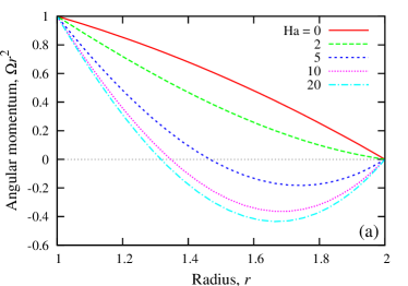
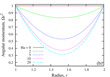
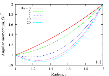
Figure 2: Angular momentum profiles for (a) $\mu=0,$ (b) $\mu=0.25,$ (c) $\mu=0.5$ and various Hartmann numbers for cylinders with $\lambda=2$ in axial magnetic field $(\beta=0)$ with no contact resistance $(\bar{\mathcal{R}}=0).$

IV Perturbed state

We consider a perturbed state

$$\left\{\begin{array}[]{c}\mbox{\boldmath$\mathrm{v}$},p\\ \mbox{\boldmath$\mathrm{j}$},\Phi\end{array}\right\}(\mbox{\boldmath$\mathrm{r}$},t)=\left\{\begin{array}[]{c}\mbox{\boldmath$\mathrm{v}$}_{0},p_{0}\\ \mbox{\boldmath$\mathrm{j}$}_{0},\Phi_{0}\end{array}\right\}(r)+\left\{\begin{array}[]{c}\mbox{\boldmath$\mathrm{v}$}_{1},p_{1}\\ \mbox{\boldmath$\mathrm{j}$}_{1},\Phi_{1}\end{array}\right\}(\mbox{\boldmath$\mathrm{r}$},t)$$

where $\mbox{\boldmath$\mathrm{v}$}_{1},$ $p_{1},$ $\mbox{\boldmath$\mathrm{j}$}_{1},$ and $\Phi_{1}$ present small-amplitude perturbations for which Eqs. (1) and (2) after linearization take the form

$$\frac{\partial\mbox{\boldmath$\mathrm{v}$}_{1}}{\partial t} + (\mbox{\boldmath$\mathrm{v}$}_{1}\cdot\mbox{\boldmath$\mathrm{\nabla}$})\mbox{\boldmath$\mathrm{v}$}_{0}+(\mbox{\boldmath$\mathrm{v}$}_{0}\cdot\mbox{\boldmath$\mathrm{\nabla}$})\mbox{\boldmath$\mathrm{v}$}_{1}$$ (6)

$$= -\frac{1}{\rho}\mbox{\boldmath$\mathrm{\nabla}$}p_{1}+\nu\mbox{\boldmath$\mathrm{\nabla}$}^{2}\mbox{\boldmath$\mathrm{v}$}_{1}+\frac{1}{\rho}\mbox{\boldmath$\mathrm{j}$}_{1}\times\mbox{\boldmath$\mathrm{B}$}_{0},$$

$$\mbox{\boldmath$\mathrm{j}$}_{1} = \sigma\left(-\mbox{\boldmath$\mathrm{\nabla}$}\Phi_{1}+\mbox{\boldmath$\mathrm{v}$}_{1}\times\mbox{\boldmath$\mathrm{B}$}_{0}\right).$$ (7)

In this paper, we focus on axisymmetric perturbations, which are typically more unstable than nonaxisymmetric ones for TC flow Rued-ANN , however this is not always the case for the conventional TD flow Chen-1993 . Analysis of nonaxisymmetric perturbations for an electromagnetically driven TD flow is outside the scope of this paper. In the axisymmetric case, the solenoidity constraints are satisfied by meridional stream functions for fluid flow and electric current as

$$\mbox{\boldmath$\mathrm{v}$}=v\mbox{\boldmath$\mathrm{e}$}_{\phi}+\mbox{\boldmath$\mathrm{\nabla}$}\times(\psi\mbox{\boldmath$\mathrm{e}$}_{\phi}),\qquad\mbox{\boldmath$\mathrm{j}$}=j\mbox{\boldmath$\mathrm{e}$}_{\phi}+\mbox{\boldmath$\mathrm{\nabla}$}\times(h\mbox{\boldmath$\mathrm{e}$}_{\phi}).$$

Note that $h$ is the azimuthal component of the induced magnetic field, which is used subsequently instead of $\Phi$ for the description of the induced current. Thus, we effectively retain the azimuthal component of the induction equation to describe meridional components of the induced current, while the azimuthal current is related explicitly to the radial velocity. In addition, for numerical purposes, we introduce also the vorticity $\mbox{\boldmath$\mathrm{\omega}$}=\mbox{\boldmath$\mathrm{\nabla}$}\times\mbox{\boldmath$\mathrm{v}$}=\omega\mbox{\boldmath$\mathrm{e}$}_{\phi}+\mbox{\boldmath$\mathrm{\nabla}$}\times(v\mbox{\boldmath$\mathrm{e}$}_{\phi})$ as an auxiliary variable. The perturbation is sought in the normal-mode form

$$\left\{v_{1},\omega_{1,}\psi_{1},h_{1}\right\}(\mbox{\boldmath$\mathrm{r}$},t)=\left\{\hat{v},\hat{\omega},\hat{\psi},\hat{h}\right\}(r)e^{\gamma t+ikz},$$

where $\gamma$ is, in general, a complex growth rate and $k$ is the axial wave number. Henceforth, we proceed to dimensionless variables by using $R_{i},$ $R_{i}^{2}/\nu,$ $R_{i}\Omega_{i},$ $B_{0},$ and $\sigma B_{0}R_{i}\Omega_{i}$ as the length, time, velocity, magnetic field, and current scales, respectively. The nondimensionalized governing equations are

$$\gamma\hat{v} = D_{k}\hat{v}-\textrm{Re}ik\left(w_{0}\hat{v}-r^{-1}\left(rv_{0}\right)^{\prime}\hat{\psi}\right)+\textrm{Ha}^{2}ik\hat{h},$$ (8)

$$\gamma\hat{\omega} = D_{k}\hat{\omega}-\textrm{Re}ik\left(w_{0}\hat{\omega}+r\left(r^{-1}w_{0}^{\prime}\right)^{\prime}\hat{\psi}-2r^{-1}v_{0}\hat{v}\right)$$ (9)

$$-\textrm{Ha}^{2}ik\left(ik\hat{\psi}+2\beta r^{-2}\hat{h}\right),$$

$$0 = D_{k}\hat{\psi}+\hat{\omega},$$ (10)

$$0 = D_{k}\hat{h}+ik\left(\hat{v}-2\beta r^{-2}\hat{\psi}\right),$$ (11)

where $D_{k}f\equiv r^{-1}\left(rf^{\prime}\right)^{\prime}-(r^{-2}+k^{2})f$ and the prime stands for $d/dr;$ $\textrm{Re}=R_{i}^{2}\Omega_{i}/\nu$ and $\textrm{Ha}=R_{i}B_{0}\sqrt{\sigma/(\rho\nu)}$ are the Reynolds and Hartmann numbers, respectively. Boundary conditions for the flow perturbation and the electric stream function on the perfectly conducting inner and outer cylinders at $r=1$ and $r=\lambda,$ respectively, are $\hat{v}=\hat{\psi}=\hat{\psi}^{\prime}=(r\hat{h})^{\prime}=0.$

The governing Eqs. (8)–(11) for perturbation amplitudes were solved in the same way as in Refs. Priede-etal-2007 and Priede-Gerbeth2008 by using a spectral collocation method on a Chebyshev-Lobatto grid with a typical number of internal points $N=32,$ which ensured the accuracy of about five digits.

The dimensionless azimuthal and axial velocity components of the base flow

$$v_{0}(r) = \bar{v}_{0}(r)+\frac{1}{2}\textrm{Ha}^{2}\bar{J}_{0}\tilde{v}_{0}(r),$$ (12)

$$w_{0}(r) = \frac{1}{2}\textrm{Ha}^{2}\bar{J}_{0}\beta\tilde{w}_{0}(r),$$ (13)

follow straightforwardly from the corresponding dimensional counterparts when $R_{i}$ and $\Omega_{i}$ are replaced by $1,$ $R_{o}$ and $\Omega_{o}$ by $\lambda=R_{o}/R_{i}$ and $\mu=\Omega_{o}/\Omega_{i},$ respectively, and $\beta_{i}$ by $\beta;$ the dimensionless counterpart of $J_{0}$ is

$$\bar{J}_{0} = \frac{J_{0}}{\sigma B_{0}\Omega_{i}R_{i}^{2}}=\left(\mu-1\right)\left(\frac{\ln\lambda}{\lambda^{-2}-1}+\frac{1}{2}\right)$$ (14)

$$\times\left(\bar{\mathcal{R}}+\ln\lambda+\frac{1}{2}\textrm{Ha}^{2}\bar{\mathcal{I}}\right)^{-1},$$

where $\bar{\mathcal{R}}=\mathcal{R}\sigma$ and $\bar{\mathcal{I}}=\mathcal{I}/R_{i}^{2}$ are the dimensionless counterparts of $\mathcal{R}$ and $\mathcal{I},$ respectively. As seen from Eqs. (12)– (14), for $\textrm{Ha}\gg 1$ velocity profiles tend to asymptotic solutions which, as noted above, depend neither on the contact resistance $\bar{\mathcal{R}}$ nor on the magnetic field strength

$$v_{0}(r) \approx \bar{v}_{0}(r)+\tilde{J}_{0}\tilde{v}_{0}(r),$$ (15)

$$w_{0}(r) \approx \tilde{J}_{0}\beta\tilde{w}_{0}(r),$$ (16)

where $\tilde{J}_{0}=\left(\mu-1\right)\left(\frac{\ln\lambda}{\lambda^{-2}-1}+\frac{1}{2}\right)/\bar{\mathcal{I}}.$

V Numerical results

V.1 Axial magnetic field

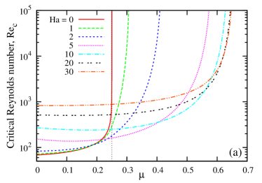
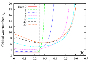
Figure 3: (a) Critical Reynolds number $Re_{c}$ and (b) wave number $k_{c}$ versus $\mu$ at various Hartmann numbers for cylinders with $\lambda=2$ and no contact resistance $(\bar{\mathcal{R}}=0)$ in purely axial magnetic field.

We start with an axial magnetic field $(\beta=0),$ for which the base flow is purely azimuthal. The profiles of angular momentum $rv_{0}(r)$ are shown in Fig. 2 for several cylinder rotation rate ratios $\mu$ and various Hartmann numbers. For $\mu=0,$ shown in Fig. 2(a), which corresponds only to the inner cylinder rotating, the profile without the magnetic field is centrifugally unstable with the angular momentum decreasing radially outward. In this case, the magnetic field slows down the overall rotation rate of the liquid making the angular momentum decrease faster at the inner cylinder that may result even in the reversal of the sense of liquid rotation at the outer cylinder when the magnetic field is sufficiently strong. This effect is due to the magnetic field trying to eliminate the differential rotation between the liquid and the endcap, which is attached to the outer cylinder and thus rotates with a lower angular velocity than the liquid above it as long as $\mu<1.$ A similar effect can also be observed in Fig. 2(b) for $\mu=0.25,$ which without the magnetic field corresponds to a marginally stable state with a constant angular momentum distribution. In this case, the magnetic field again retards the liquid rotation so rending the distribution of angular momentum centrifugally unstable at the inner cylinder and stable at the outer one. For $\mu=0.5$ shown in Fig. 2(c), the profile without magnetic field is centrifugally stable with the angular momentum increasing radially outward. However, a strong enough magnetic field changes the distribution of the angular momentum at the inner cylinder from radially increasing to decreasing one so rending the profile centrifugally unstable.

This is confirmed by the critical Reynolds number plotted against $\mu$ for various Hartmann numbers in Fig. 3(a) with the corresponding critical wave numbers shown in Fig. 3(b). As seen in Fig. 3(a), without magnetic field $(\textrm{Ha}=0),$ the critical Reynolds number tends to infinity as $\mu$ approaches the Rayleigh line $\mu_{c}=\lambda^{-2}=0.25$ defined by $d\left(r^{2}\Omega\right)/dr=0,$ at which the profile of angular momentum becomes centrifugally stable. As the magnetic field is increased, the instability starts to extend beyond the Rayleigh line reaching $\mu\approx 0.65$ at sufficiently large Hartmann numbers. Although this extension of the instability beyond the Rayleigh line may look like an MRI, it has a principally different physical mechanism. Namely, in the MRI, the magnetic field destabilizes the flow without altering it, whereas here the magnetic field does alter the base flow by rendering it centrifugally unstable as discussed above. Moreover, the standard MRI in axial magnetic field is not captured by the inductionless approximation $(\textrm{Pm}=0)$ used here Herron-Goodman-2006 . Thus, in axial magnetic field, this centrifugal instability occurring beyond the Rayleigh line can easily be distinguished from the true MRI.

V.2 Helical magnetic field

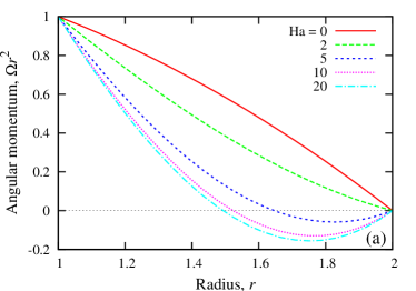
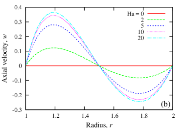
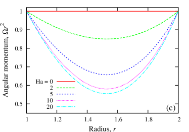
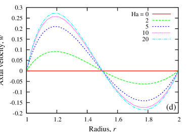
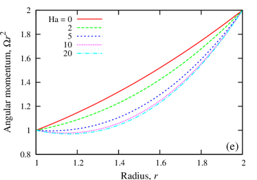
Figure 4: [(a), (c), and (e)] Radial profiles of angular momentum and [(b), (d), and (f)] axial velocity for [(a) and (b)] $\mu=0$ , [(c) and (b)] $\mu=0.25,$ [(e) and (f)] $\mu=0.5$ and various Hartmann numbers for cylinders with $\lambda=2$ and no contact resistance $(\bar{\mathcal{R}}=0)$ in helical magnetic field with $\beta=6.$

As seen in Fig. 4, in a helical magnetic field, the base flow besides the azimuthal component has also an axial one, which is driven by the interaction of radial current with the azimuthal component of magnetic field. In the configuration with the endcap attached to a slower-rotating outer wall, the induced electric current is flowing radially outward, as discussed above and, thus, the resulting axial electromagnetic force is directed upward. Because both the current and azimuthal magnetic field decrease radially outward as $\sim 1/r,$ the resulting electromagnetic force is stronger at the inner wall, where it drives the liquid upward as seen in Figs. 4(b), 4(d), and 4(f). Since the annular gap is supposed to be closed at both ends, the constant axial pressure gradient arising in the response to the electromagnetic force drives a return flow along the outer cylinder, which compensates for the upward one along the inner cylinder. This axial flow in the azimuthal magnetic field, in turn, induces an additional electrostatic potential, which contributes to that induced by the azimuthal flow in the axial field as described by Eq. (3). The total potential difference induced by the flow between the inner and outer cylinders balances that induced by the rotation of bottom in the axial magnetic field, which is given by Eq. (4). The potential balance determines the magnitude of the induced radial current defined by Eq. (5), which, in turn, interacts with the magnetic field and disturbs the flow. Thus, the perturbation of the azimuthal flow is weaker in helical magnetic field than it is in a purely axial one because a part of the potential difference is compensated by the axial flow [see Figs. 2, 4(a), 4(c), and 4(e)].

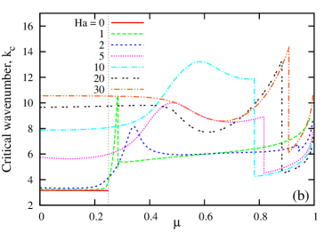
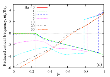
Figure 5: (a) Critical Reynolds number $Re_{c},$ (b) wave number $k_{c}$ and (c) the rescaled frequency $\omega_{c}/Re_{c}$ versus $\mu$ at various Hartmann numbers for cylinders with $\lambda=2$ and no contact resistance $(\bar{\mathcal{R}}=0)$ in helical magnetic field with $\beta=6.$

The instability characteristics in a helical magnetic field plotted in Fig. 5 differ considerably from those in axial magnetic field shown in Fig. 3. In contrast to the axial magnetic field, now the most unstable mode of instability is oscillatory, i.e., a traveling wave as for the HMRI. However, it is important to note that the phase velocity of this wave, which is determined by the sign of the frequency shown in Fig. 5(c), is directed upward oppositely to that of true HMRI. The reversed phase velocity is due to the longitudinal flow, which is absent for the ideal HMRI with electrically decoupled cylinders. As seen in Figs. 4(a), 4(c), and 4(e), the radial current interacting with the axial component of the magnetic field causes the angular momentum to decrease radially outward at the inner cylinder that renders the flow centrifugally unstable. Furthermore, the Taylor vortices arising at the inner cylinder are advected by the longitudinal flow upward. The advection in this case obviously dominates over the direct electromagnetic effect of helical magnetic field, which would drive the true HMRI wave in the opposite direction.

Moreover, in a helical magnetic field in contrast to purely axial one, the instability is seen to extend much farther beyond the Rayleigh line up to the limit of solid-body rotation defined by $\mu=1$ and even beyond it, which is not considered here. The instability in helical magnetic field differs significantly from that in purely axial field. As seen in Fig. 5, for $\textrm{Ha}=1,$ shortly after the Rayleigh line, the most unstable mode switches from the initial Taylor vortices branch to another one, which is obviously associated with the axial flow. For larger Hartmann numbers, this transition proceeds smoothly with the critical wave number developing a maximum at certain $\mu$ when $\textrm{Ha}\lesssim 10.$ Beyond the Rayleigh line, the critical Reynolds number first decreases with the Hartmann number up to $\textrm{Ha}\approx 10$ and then starts to grow for larger Ha again. For larger $\mu,$ the most unstable mode jumps to another branch with a considerably smaller critical wave number and positive frequency, which corresponds to the opposite direction of the phase velocity now coinciding with that of the true HMRI. Note that such jumps of the critical mode are characteristic also for the conventional TD flow DiPrima-1959 ; Hughes-Reid-1964 .

VI Summary and conclusions

We have considered linear stability of a TD-type flow of an electrically conducting liquid in the annulus between two infinitely long perfectly conducting and differentially rotating cylinders in the presence of a generally helical magnetic field. The cylinders were supposed to be electrically connected through a remote endcap. We showed that this electrical connection can render the base flow hydrodynamically unstable. First, the azimuthal base flow in an axial magnetic field gives rise to a radial emf. If the cylinders are electrically decoupled, no current can close between them, and, consequently, the emf results in the radial charge redistribution, which gives rise to the electrostatic potential whose gradient compensates the original emf. If there is no current, there is no electromagnetic force and no effect of the magnetic field on the base flow either. This corresponds to the ideal TC flow, which is used as a reference for the definition of MRI, where the magnetic field is expected to destabilize the base flow by affecting only its disturbances but not the base flow itself.

This is no longer the case when the cylinders are electrically connected, and a radial current can close between them. The interaction of radial current with the axial component of the magnetic field gives rise to the azimuthal electromagnetic force, which tries eliminate the velocity difference between the endcap and the liquid above it. Depending on the strength of magnetic field and the effective contact resistance between the inner and outer cylinder, this electromagnetic force can modify the profile of azimuthal base flow so that it becomes centrifugally unstable. As a result, the magnetic field makes the instability extend significantly beyond its apparent Rayleigh line so resembling MRI in the case of an unperturbed TC flow. Furthermore, in a helical magnetic field, the interaction of radial current with the azimuthal component of magnetic field gives rise to an axial electromagnetic force, which drives a longitudinal flow. First, this longitudinal flow going upward along the inner cylinder, where the azimuthal base flow is destabilized by the magnetic field, advects Taylor vortices, so giving rise to a traveling wave as in helical MRI. However, the direction of the most unstable traveling wave of this centrifugal instability is opposite to that of the true MRI. Second, for sufficiently large differential rotation, the longitudinal flow becomes hydrodynamically unstable itself. For electrically connected cylinders in helical magnetic field, hydrodynamic instability is possible at any sufficiently large differential rotation. In this case, there is no pure hydrodynamic stability limit defined in the terms of the critical ratio of rotation rates of inner and outer cylinders that would allow one to discriminate between magnetically modified hydrodynamic instability and the HMRI.

From the experimental point of view, a crucial test for the pseudo–MRI would be the extension of the Taylor vortex flow beyond the Rayleigh line in purely axial magnetic field at $\textrm{Rm}\lesssim 1.$ The PROMISE experiment reports only one such apparently successful test in which, however, the time-averaged flow and thus stationary Taylor vortices, if any, are removed Rued-apjl . Traveling wave appears as soon as the azimuthal component of the field is switched on. As to the helical magnetic field, the experiment Stefani-NJP seems to find the right direction of the phase velocity in agreement with the ideal HMRI model rather than that of the pseudo–MRI considered in this paper. But this does not necessarily mean that the real base flow in the experiment is any closer to the ideal TC one. Note that the nonaxisymmetric $m=1$ instability mode unexpectedly observed in the PROMISE experiment is characteristic for certain regimes of the conventional TD flow Chen-1993 .

Although the current circulation through the liquid metal has been eliminated in a modified PROMISE experimentStefani-etal2009a by insulating the inner cylinder, the base flow still remains strongly affected by the Ekman pumping due to the endcaps which makes it more complex than the one used in this study. In the new PROMISE-2 setup Stefani-etal2009b ; Stefani-etal2009c , the Ekman pumping has been significantly reduced by using split rings for the endcap, which is insulating now, and thus prevents the current circulation through it. Although the instabilities appear much sharper in the new setup than in the previous one, the actual hydrodynamic stability limit, if any, of the base flow and so the nature of the observed instabilities is still unclear. In particular, as shown by Szklarski and Rüdiger Szklarski-Ruediger2007 , the base flow may significantly be affected by the magnetic field also when the endcaps are insulating provided that $\textrm{Ha}\gtrsim 10.$

In conclusion, it is not appropriate to use the Rayleigh line of the ideal TC flow as a criterion to determine the MRI in a significantly different flow. More elaborate numerical analysis may be necessary for this purpose.

- (1) S. A. Balbus and J. F. Hawley, Astrophys. J. 376, 214 (1991);
- (2) S. A. Balbus and J. F. Hawley, Rev. Mod. Phys. 70, 1 (1998).
- (3) E. P. Velikhov, Sov. Phys. JETP 36, 995 (1959).
- (4) S. Chandrasekhar, Proc. Nat. Acad. Sci. 46, 253 (1960); Hydrodynamic and Hydromagnetic Stability, (Oxford University, London, 1961), Sec. 81.
- (5) D. R. Sisan, N. Mujica, W. A. Tillotson, Y.-M. Huang, W. Dorland, A. B. Hassam, T. M. Antonsen, and D. P. Lathrop, Phys. Rev. Lett. 93, 114502 (2004).
- (6) H. Ji, M. Burin, E. Schartman, and J. Goodman, Nature 444, 343 (2006).
- (7) J. Goodman and H. Ji, J. Fluid. Mech. 462, 365 (2002).
- (8) R. Hollerbach and G. Rüdiger, Phys. Rev. Lett. 95, 124501 (2005).
- (9) G. Rüdiger, R. Hollerbach, F. Stefani, Th. Gundrum, G. Gerbeth, and R. Rosner, Astrophys. J. 649, L145 (2006).
- (10) F. Stefani, Th. Gundrum, G. Gerbeth, G. Rüdiger, M. Schultz, J. Szklarski, and R. Hollerbach, Phys. Rev. Lett 97, 184502 (2006).
- (11) F. Stefani, Th. Gundrum, G. Gerbeth, G. Rüdiger, J. Szklarski, and R. Hollerbach, New J. Phys. 9, 295 (2007).
- (12) W. Liu, J. Goodman, I. Herron, and H. Ji, Phys. Rev. E 74, 056302 (2006).
- (13) W. Liu, J. Goodman, and H. Ji, Phys. Rev. E 76, 016310 (2007).
- (14) J. Szklarski, Astron. Nachr. 328, 499 (2007).
- (15) W. Liu, Phys. Rev. E 77, 056314 (2008).
- (16) J. Priede and G. Gerbeth, Phys. Rev. E 79, 046310 (2009); e-print arXiv:0810.0386.
- (17) J. Szklarski and G. Rüdiger, Rev. E 76, 066308 (2007).
- (18) J. Priede, I. Grants, and G. Gerbeth, Phys. Rev. E 75, 047303 (2007).
- (19) E. P. Velikhov, A. A. Ivanov, S. V. Zakharov, V. S. Zakharov, A. O. Livadny, and K. S. Serebrennikov, Phys. Lett. A 358, 216 (2006).
- (20) I. V. Khalzov, V. I. Ilgisonis, A. I. Smolyakov, and E. P. Velikhov, Phys. Fluids 18, 124107 (2006).
- (21) S. Chandrasekhar, Hydrodynamic and Hydromagnetic Stability, (Oxford University, London, 1961), Sec. 76.
- (22) G. Rüdiger, R. Hollerbach, M. Schultz, and D. A. Shalybkov, Astron. Nachr. 326, 409 (2005).
- (23) F. Chen, Phys. Rev. E 48, 1036 (1993).
- (24) I. Herron and J. Goodman, Z. Angew. Math. Phys. 57, 615 (2006).
- (25) R. C. DiPrima, J. Fluid Mech. 6, 462 (1959).
- (26) T. H. Hughes and W. H. Reid, Z. Angew. Math. Phys. 15, 573 (1964).
- (27) F. Stefani, G. Gerbeth, Th. Gundrum, J. Szklarski, G. Rüdiger, and R. Hollerbach, Astron. Nachr. 329, 652 (2008);
- (28) F. Stefani, G. Gerbeth, Th. Gundrum, J. Szklarski, G. Rüdiger, and R. Hollerbach, e-print arXiv:0812.3790.
- (29) F. Stefani, G. Gerbeth, Th. Gundrum, R. Hollerbach, J. Priede, G. Rüdiger, and J. Szklarski, e-print arXiv:0904.1027.