Flavour Violation in Anomaly Mediated Supersymmetry Breaking

Abstract:

We study squark flavour violation in the anomaly mediated supersymmetry broken (AMSB) minimal supersymmetric standard model. Analytical expressions for the three-generational squark mass matrices are derived. We show that the anomaly-induced soft breaking terms have a decreasing amount of squark flavour violation when running from the GUT to the weak scale. Taking into account inter-generational squark mixing, we work out non-trivial constraints from $B\rightarrow X_{s}\gamma$ and $B_{s}\to\mu\mu$, which complement each other, as well as $B\to\tau\nu$ decays. We further identify a region of parameter space where the anomalous magnetic moment of the muon and the $B\rightarrow X_{s}\gamma$ branching ratio are simultaneously accommodated. Since anomaly mediation is of the minimal flavour-violating type, the generic flavour predictions for this class of models apply, including a CKM-induced (and hence small) $B_{s}-\bar{B}_{s}$-mixing phase.

1 Introduction

Increasing precision in the calculation of sparticle effects is an important part of theoretical preparation for the LHC. Much of this work has concentrated on the mSUGRA scenario, where it is assumed that the unification of gauge couplings at high energies is accompanied by a corresponding unification in both the soft supersymmetry-breaking $\phi^{*}\phi$ scalar masses and the gaugino masses: and also that the cubic scalar $\phi^{3}$ interactions are of the same form as the Yukawa couplings and related to them by a common constant of proportionality, the $A$ parameter.

Anomaly mediation (AMSB) [1]–​[16] as the main source of supersymmetry breaking is an attractive alternative to the mSUGRA paradigm. In AMSB, the $\phi^{*}\phi$ masses, $\phi^{3}$ couplings and gaugino masses are all determined by the appropriate power of the gravitino mass multiplied by perturbatively calculable functions of the dimensionless couplings of the underlying supersymmetric theory. Moreover these functions are renormalisation group (RG) invariant, and the AMSB predictions are thus ultraviolet insensitive [8]. Unfortunately the theory in its simplest form leads to tachyonic sleptons and thus fails to accommodate the usual electroweak vacuum state. There are many different successful approaches which fix this problem, however.

There have been a number of studies of the sparticle spectrum in the AMSB context but these have generally been carried out in the approximation whereby third-generation Yukawa couplings only are retained. In this paper we consider flavour physics in the AMSB context; aspects of this were considered in Ref. [5] for the $b\to s\gamma$ process, but there has been considerable progress both on the experimental and theoretical side since then. We will also show how AMSB satisfies the requirements of the principle of Minimal Flavour Violation (MFV) [17]–​[20]. Moreover, we will show that specific to AMSB there is a natural suppression of flavour changing neutral current (FCNC) effects related to the size of the top quark Yukawa coupling at the electroweak scale.

We consider in some detail the critical calculation of the $B\rightarrow X_{s}\gamma$ branching ratio, taking into account inter-generational squark mixing. We show that for positive Higgs mass term $\mu$ the dependence of ${\rm BR}(B\rightarrow X_{s}\gamma)$ on $\tan\beta$, the ratio of the two Higgs vacuum expectation values, is positively dramatic, because the charged Higgs mass has a minimum for large $\tan\beta$ in the class of AMSB models we are treating. As a result, for $\mu>0$, $B\rightarrow X_{s}\gamma$ constrains $\tan\beta$ to be relatively low; we nevertheless show that within AMSB models it is possible for the supersymmetric contribution to account for the current discrepancy between theory and experiment for the muon anomalous magnetic moment. We further analyse leptonic $B_{s}\to\mu\mu$ and $B\to\tau\nu$ decays within AMSB. For $B_{s}\to\mu\mu$ we take into account the full flavour structure of the squark sector and include both chargino and gluino contributions. Despite AMSB being MFV, the gluino contributions induced by inter-generational down-squark mixing turn out to be significant. We show that current data on the leptonic modes are beginning to probe the $\mu<0$ branch. Once higher statistics become available these decays could provide decisive constraints on the parameter space.

The plan of the paper is as follows: In Section 2 we review AMSB and squark flavour violation in minimal supersymmetric models. We present in Section 3 analytical results for the AMSB soft terms with full generational structure, showing thereby how AMSB fulfils the MFV principle. We also assess the effect on the squark mass spectrum of a number of solutions to the tachyonic slepton problem. In Section 4 we give numerical estimates for the size of the flavour-mixing entries of the squark mass matrices. We further evaluate the constraints from the $B\to X_{s}\gamma$ decay, work out implications for leptonic $B$-decay observables in AMSB and comment on the anomalous magnetic moment of the muon. In Section 5 we conclude. In Appendix A we provide details on the numerical computation of the squark flavour-mixing parameters.

2 Generalities

We review AMSB in Section 2.1 and general squark flavour violation within the MSSM in Section 2.2.

2.1 Anomaly mediated supersymmetry breaking

For completeness and to establish notation, let us recapitulate some standard results for the general case. We take an ${\cal N}=1$ supersymmetric gauge theory with gauge group $\Pi_{\alpha}G_{\alpha}$ and with superpotential

$$W(\Phi)={\textstyle{\frac{1}{6}}}Y^{ijk}\Phi_{i}\Phi_{j}\Phi_{k}+{\textstyle{\frac{1}{2}}}\mu^{ij}\Phi_{i}\Phi_{j}.$$ (1)

We also include the soft supersymmetry-breaking terms

$${\cal{L}}_{\rm soft}=-(m^{2})^{j}{}_{i}\phi^{i}\phi_{j}-\left({\textstyle{\frac{1}{6}}}h^{ijk}\phi_{i}\phi_{j}\phi_{k}+{\textstyle{\frac{1}{2}}}b^{ij}\phi_{i}\phi_{j}+{\textstyle{\frac{1}{2}}}M_{\alpha}\lambda_{\alpha}\lambda_{\alpha}+{\rm h.c.}\right),$$ (2)

where we denote by $\phi$ the scalar component of the superfield $\Phi$ and $\phi^{i}=(\phi_{i})^{*}$. Here $M_{\alpha}$ are the gaugino masses and $h$, $b$ and $m^{2}$ are the standard soft supersymmetry-breaking scalar terms.

The following set of results for soft supersymmetry-breaking terms are characteristic of AMSB and are RG invariant [4]:

$$M_{\alpha} = m_{3/2}\beta_{g_{\alpha}}/g_{{\alpha}},$$ (3a)

$$h^{ijk} = -m_{3/2}\beta^{ijk}_{Y},$$ (3b)

$$(m^{2})^{i}{}_{j} = \frac{1}{2}m_{3/2}^{2}\mu\frac{d}{d\mu}\gamma^{i}{}_{j},$$ (3c)

$$b^{ij} = \kappa m_{3/2}\mu^{ij}-m_{3/2}\beta_{\mu}^{ij}.$$ (3d)

where $\gamma^{i}{}_{j}$ is the chiral superfield anomalous dimension matrix, and $\beta_{g_{\alpha}}$, $\beta_{Y}$ are the $\beta$-functions for the gauge and Yukawa couplings, respectively. $\beta_{Y}$ is given by

$$\beta^{ijk}_{Y}=\gamma^{i}{}_{l}Y^{ljk}+\gamma^{j}{}_{l}Y^{ilk}+\gamma^{k}{}_{l}Y^{ijl},$$ (4)

and $\beta_{\mu}$ by a similar expression. At one loop we have

$$16\pi^{2}\beta_{g_{\alpha}}^{(1)} = g_{\alpha}^{3}\left[T(R_{\alpha})-3C(G_{\alpha})\right],$$ (5a)

$$16\pi^{2}\gamma^{(1)i}{}_{j} = {\textstyle{\frac{1}{2}}}Y^{ikl}Y_{jkl}-2\sum_{\alpha}g_{\alpha}^{2}[C(R_{\alpha})]^{i}{}_{j}.$$ (5b)

Here $R_{\alpha}$ is the group representation for $G_{\alpha}$ acting on the chiral fields, $C(R_{\alpha})$ the corresponding quadratic Casimir and $T(R_{\alpha})=(r_{\alpha})^{-1}{\rm Tr}[C(R_{\alpha})]$ , $r_{\alpha}$ being the dimension of $G_{\alpha}$. For the adjoint representation, $C(R_{\alpha})=C(G_{\alpha})I_{\alpha}$, where $I_{\alpha}$ is the $r_{\alpha}\times r_{\alpha}$ unit matrix. Obviously if the gauge group has an abelian factor, $G_{1}$ say, with hypercharge matrix ${\cal Y}^{i}{}_{j}={\cal Y}_{i}\delta^{i}{}_{j}$, then $T(R_{1})={\rm Tr}[{\cal Y}^{2}]$, $\left[C(R_{1})\right]^{i}{}_{j}=({\cal Y}^{2})^{i}{}_{j}$ and $C(G_{1})=0$.

As we indicated in the introduction, Eq. (3c) is unrealistic for the sleptons; most phenomenology has been done by replacing it (at the GUT scale) with

$$({\overline{m}}^{2})^{i}{}_{j}=\frac{1}{2}m_{3/2}^{2}\mu\frac{d}{d\mu}\gamma^{i}{}_{j}+m_{0}^{2}\delta^{i}{}_{j},$$ (6)

that is, by introducing a common scalar mass for the chiral super multiplets. We will call this model mAMSB in what follows. There have been a number of alternative approaches to the problem; for a discussion see in particular Ref. [2], and for the phenomenology of deflected anomaly mediation see Ref. [6].

One approach, first explored in detail in Ref. [7], and subsequently by a number of authors [8]–​[13], is to replace Eq. (3c) with

$$({\overline{m}}^{2})^{i}{}_{j}=\frac{1}{2}m_{3/2}^{2}\mu\frac{d}{d\mu}\gamma^{i}{}_{j}+\xi{\cal Y}_{i}\delta^{i}{}_{j},$$ (7)

where $\xi$ is a constant (with dimensions of $\hbox{mass}^{2}$) and ${\cal Y}_{i}$ are charges corresponding to a $U(1)$ symmetry of the theory. The $\xi{\cal Y}$ term corresponds in form to a Fayet-Iliopoulos (FI) $D$-term. This alternative has the advantage that it does not require us to postulate an independent source of supersymmetry breaking characterised by $m_{0}^{2}$; the new term in Eq. (7) can be derived in a natural way via the spontaneous breaking of a $U(1)$ symmetry at high energies [14, 15].

For a discussion of how Eq. (7) affects the RG invariance of the AMSB expressions see Ref. [16]. The outcome is that if we work at a specific renormalisation scale (such as $M_{{\scriptscriptstyle\rm SUSY}}$) throughout, then we may use Eq. (7), with a specific value of $\xi$, as long as the $U(1)$ represented by the charges ${\cal Y}$ has no mixed anomalies with the SM gauge group.

An example of a way to provide a viable solution to this slepton problem but retain Eq. (3c) unaltered is to introduce $R$-parity violating leptonic interactions, which provide positive sleptonic $(\hbox{mass})^{2}$ contributions [21].

Most applications of AMSB to the minimal supersymmetric standard model (MSSM) and variants have employed Eq. (3a), (3b) and Eq. (6) or (7), and determined the Higgs $B$ parameter (along with the $\mu$ term) by the minimisation of the scalar potential. This reflects the fact that the form of the $B$-term is more model dependent than the other soft breaking terms; for a recent discussion see Ref. [15]. In fact Eq. (3d) (with the arbitrary parameter $\kappa$) is the most general form consistent with RG invariance of the AMSB form of soft supersymmetry breaking.

The MSSM (with right-handed neutrino superfields $\bar{\nu}$) admits two independent, generation-blind and anomaly-free $U(1)$ symmetries, one of which is of course $U(1)_{Y}$; it is convenient for our purposes to parameterise them with the lepton doublet and singlet charges. The possible charge assignments are shown in Table 1; we will call the additional symmetry $U(1)^{\prime}$ in what follows. Note that in the effective theory below the scale of the right-handed neutrino mass $U(1)^{\prime}$ has no mixed anomalies with the SM gauge group.

$Q$	${\bar{U}}$	${\bar{D}}$	$H_{1}$	$H_{2}$	${\bar{\nu}}$
$-\frac{1}{3}L$	$-e-\frac{2}{3}L$	$e+\frac{4}{3}L$	$-e-L$	$e+L$	$-2L-e$

Table 1: Anomaly-free $U(1)^{\prime}$ charges for arbitrary lepton doublet and singlet charges $L$ and $e$ respectively. $U(1)_{Y}$ corresponds to $L=-1/2$ and $e=1$. $\bar{\nu}$ is a SM gauge singlet.

$Q,{\bar{U}}$	${\bar{D}}$	$\bar{\nu}$	$H_{1}$	$H_{2}$	$N$
$e$	$L$	$2e-L$	$-2e$	$-e-L$	$L+3e$

Table 2: Anomaly-free $U(1)_{SU(5)}$ charges for arbitrary lepton doublet and singlet charges ($L$ and $e$ respectively) compatible with $SU(5)\times U(1)$. $N$, $\bar{\nu}$ are SM gauge singlets.

Alternatively, by introducing an additional SM gauge singlet $N$ per generation, appropriately charged under the $U(1)$ symmetry, and completing the two Higgs multiplets to a $5$ and a ${\overline{5}}$ (per generation) we can have a charge assignment that is compatible with grand unification to $SU(5)\times U(1)$ (see Table 2). When we assess this possibility we will assume that only one pair of Higgs doublets (and no Higgs triplets) survive in the effective field theory below unification. So this case differs from the $U(1)^{\prime}$ case in that the $U(1)_{SU(5)}$ is anomalous in the low-energy theory; this will affect the discussion of the RG invariance of the soft terms in what follows.

2.2 Flavour structure of the MSSM Lagrangian

The quark chiral superfields of the MSSM have the following $G_{SM}=SU(3)_{c}\times SU(2)_{L}\times U(1)_{Y}$ quantum numbers in the SLHA2 [22] conventions, which we adopt:

$$Q:\,(3,2,{\textstyle{\frac{1}{6}}}),\quad{\bar{U}}:\,({\bar{3}},1,-{\textstyle{\frac{2}{3}}}),\quad{\bar{D}}:({\bar{3}},1,{\textstyle{\frac{1}{3}}}),$$ (8)

and the superpotential of the MSSM is written as

$$W_{Q} = \epsilon_{ab}\left[Q_{i}^{b}\,(Y_{D})_{ij}\,H_{1}^{a}\,{\bar{D}}_{j}+L_{i}^{b}\,(Y_{E})_{ij}\,H_{1}^{a}\,{\bar{E}}_{j}+Q_{i}^{a}\,(Y_{U})_{ij}\,H_{2}^{b}\,{\bar{U}}_{j}-\mu H_{1}^{a}H_{2}^{b}\right].$$ (9)

Throughout this section, we denote $SU(2)_{L}$ fundamental representation indices by $a,b=1,2$ and the generation indices by $i,j=1,2,3$. $\epsilon_{ab}=\epsilon^{ab}$ is the totally antisymmetric tensor, with $\epsilon_{12}=1$. The $SU(3)$ colour indices are suppressed. All MSSM running parameters are in the $\rm{\overline{DR}}$ scheme [23]. We now tabulate the notation of the relevant soft supersymmetry (SUSY) breaking parameters. The squark trilinear scalar interaction potential is

$$V_{3}=\epsilon_{ab}\left[\tilde{Q}_{i_{L}}^{b}\,(T_{D})_{ij}\,\tilde{d}^{*}_{jR}\,H_{1}^{a}+\tilde{Q}_{i_{L}}^{a}\,(T_{U})_{ij}\,\tilde{u}^{*}_{jR}\,H_{2}^{b}\right]+{\rm h.c.},$$ (10)

where fields with a tilde are the scalar components of the superfield with the identical capital letter. Note that the electric charges of ${\tilde{u}}_{R}$, ${\tilde{d}}_{R}$ are +2/3 and -1/3 respectively. The squark bilinear SUSY-breaking terms are contained in the potential

$$V_{2}={\tilde{Q}^{*}}_{iLa}\,(m_{\tilde{Q}}^{2})_{ij}\,\tilde{Q}_{jL}^{a}+\tilde{u}_{iR}\,(m_{\tilde{u}}^{2})_{ij}\,{\tilde{u}^{*}}_{jR}+\tilde{d}_{iR}\,(m_{\tilde{d}}^{2})_{ij}\,{\tilde{d}^{*}}_{jR}.$$ (11)

Eqs. (9)–(11) are in the basis of flavour eigenstates. To discuss flavour violation we need to work in the so-called super-CKM basis, where the quark mass matrices are diagonal and the squarks are rotated parallel to their fermionic partners. We choose the following convention for the Yukawa couplings and for the CKM matrix $V$:

$$Y_{U}=V^{T}\mbox{diag}(\lambda_{u},\lambda_{c},\lambda_{t}),\qquad Y_{D}=\mbox{diag}(\lambda_{d},\lambda_{s},\lambda_{b}),$$ (12)

where $\lambda_{q}$ denote the Yukawa couplings of the quarks in the mass eigenstate basis. Under this convention the down-type $SU(2)_{L}$-doublet squarks and the singlets are already in the super-CKM basis, while the up-type doublets need to be rotated. We define the $6\times 6$ mass matrices for the up-type and down-type squarks as

$${\cal L}^{\rm mass}_{\tilde{q}}~{}=~{}-\Phi_{u}^{\dagger}\,{\cal M}_{\tilde{u}}^{2}\,\Phi_{u}-\Phi_{d}^{\dagger}\,{\cal M}_{\tilde{d}}^{2}\,\Phi_{d}~{},$$ (13)

where $\Phi_{u}=(\tilde{u}_{L},\tilde{c}_{L},\tilde{t}_{L},\tilde{u}_{R},\tilde{c}_{R},\tilde{t}_{R})^{T}$ and $\Phi_{d}=(\tilde{d}_{L},\tilde{s}_{L},\tilde{b}_{L},\tilde{d}_{R},\tilde{s}_{R},\tilde{b}_{R})^{T}$. The mass matrices read

$${\cal M}_{\tilde{u}}^{2} = \left(\begin{array}[]{cc}m^{2}_{\tilde{U}_{L}}+m^{2}_{u}+D_{u\,LL}{}{}{}&\frac{v_{2}}{\sqrt{2}}\,{\widehat{T}}_{U}^{\dagger}-\mu\,m_{u}\,\cot\beta\\ \\ \frac{v_{2}}{\sqrt{2}}\,{\widehat{T}}_{U}-\mu^{*}\,m_{u}\,\cot\beta{}{}{}&{{m}^{2}_{\tilde{u}}}^{T}+m^{2}_{u}+D_{u\,RR}\\ \end{array}\right)\,\,,$$ (17)

$${\cal M}_{\tilde{d}}^{2} = \left(\begin{array}[]{cc}m^{2}_{\tilde{D}_{L}}+m^{2}_{d}+D_{d\,LL}{}{}{}&\frac{v_{1}}{\sqrt{2}}\,{T}_{D}^{*}-\mu\,m_{d}\,\tan\beta\\ \\ \frac{v_{1}}{\sqrt{2}}\,{T}_{D}^{T}-\mu^{*}\,m_{d}\,\tan\beta{}{}{}&{m^{2}_{\tilde{d}}}^{T}+m^{2}_{d}+D_{d\,RR}\\ \end{array}\right)\,\,.$$ (21)

In the equations above, $v_{1}$ and $v_{2}$ are the vacuum expectation values (VEVs) of the two Higgs doublets (with $\tan\beta\equiv v_{2}/v_{1}$ and $v\equiv\sqrt{v_{1}^{2}+v_{2}^{2}}\approx 246$ GeV), the matrices $m_{q}$ (with $q=u,d$) are the diagonal quark masses and $D_{q\,LL,RR}$ are flavour-diagonal D-term contributions. Furthermore, $m^{2}_{\tilde{D}_{L}}\equiv{m_{\tilde{Q}}^{2}}$, and we introduced the $3\times 3$ matrices

$$m^{2}_{\tilde{U}_{L}}\equiv V\,{m}_{\tilde{Q}}^{2}\,V^{\dagger}\,,~{}~{}~{}{\widehat{T}_{U}}\equiv T_{U}^{T}\,V^{\dagger}\,,$$ (22)

accounting for the rotation of the up-type doublets to the super-CKM basis.

3 AMSB Squark Flavour

We derive and analyse the exact one-loop AMSB squark soft terms with the full three-generational structure in Section 3.1. We then go on to show how the soft terms are in MFV form in Section 3.2. In Section 3.3 we discuss the implications of various solutions to the tachyonic slepton mass problem for the squark sector.

3.1 Fully flavoured squark mass boundary conditions

The one-loop anomalous dimensions for the quark and Higgs chiral superfields are easily derived from Eq. (5b) and are given by

$$(16\pi^{2})\gamma_{Q}^{T} = Y_{U}Y_{U}^{\dagger}+Y_{D}Y_{D}^{\dagger}-\left({\textstyle{\frac{1}{30}}}g_{1}^{2}+{\textstyle{\frac{3}{2}}}g_{2}^{2}+{\textstyle{\frac{8}{3}}}g_{3}^{2}\right).\mathbf{1}\,,$$ (23a)

$$(16\pi^{2})\gamma_{U} = 2Y_{U}^{\dagger}Y_{U}-\left({\textstyle{\frac{8}{15}}}g_{1}^{2}+{\textstyle{\frac{8}{3}}}g_{3}^{2}\right).\mathbf{1}\,,$$ (23b)

$$(16\pi^{2})\gamma_{D} = 2Y_{D}^{\dagger}Y_{D}-\left({\textstyle{\frac{2}{15}}}g_{1}^{2}+{\textstyle{\frac{8}{3}}}g_{3}^{2}\right).\mathbf{1}\,,$$ (23c)

$$(16\pi^{2})\gamma_{H_{2}} = 3{\rm Tr}\left(Y_{U}^{\dagger}Y_{U}\right)-{\textstyle{\frac{3}{10}}}g_{1}^{2}-{\textstyle{\frac{3}{2}}}g_{2}^{2}\,,$$ (23d)

$$(16\pi^{2})\gamma_{H_{1}} = 3{\rm Tr}\left(Y_{D}^{\dagger}Y_{D}\right)+{\rm Tr}\left(Y_{E}^{\dagger}Y_{E}\right)-{\textstyle{\frac{3}{10}}}g_{1}^{2}-{\textstyle{\frac{3}{2}}}g_{2}^{2}\,,$$ (23e)

where $\mathbf{1}$ is the identity matrix in flavour space. The quark Yukawa $\beta$ functions are

$$\beta_{Y_{U}}=Y_{U}\gamma_{U}+(\gamma_{Q}^{T}+\gamma_{H_{2}})Y_{U},\quad\beta_{Y_{D}}=Y_{D}\gamma_{D}+(\gamma_{Q}^{T}+\gamma_{H_{1}})Y_{D},\\$$ (24)

from which expressions we obtain using Eq. (3c) the following leading-order results:

$$\frac{(16\pi^{2})^{2}(m_{\tilde{Q}}^{2})^{T}}{m_{3/2}^{2}} = \left(-{\textstyle{\frac{11}{50}}}g_{1}^{4}-{\textstyle{\frac{3}{2}}}g_{2}^{4}+8g_{3}^{4}\right).\mathbf{1}+(Y_{U}Y_{U}^{\dagger})\left(3\mbox{Tr}(Y_{U}Y_{U}^{\dagger})-{\textstyle{\frac{13}{15}}}g_{1}^{2}-3g_{2}^{2}-{\textstyle{\frac{16}{3}}}g_{3}^{2}\right)$$ (25a)

$$+ (Y_{D}Y_{D}^{\dagger})\left(3\mbox{Tr}(Y_{D}Y_{D}^{\dagger})+\mbox{Tr}(Y_{E}Y_{E}^{\dagger})-{\textstyle{\frac{7}{15}}}g_{1}^{2}-3g_{2}^{2}-{\textstyle{\frac{16}{3}}}g_{3}^{2}\right)$$

$$+ Y_{U}Y_{U}^{\dagger}Y_{D}Y_{D}^{\dagger}+Y_{D}Y_{D}^{\dagger}Y_{U}Y_{U}^{\dagger}+3(Y_{U}Y_{U}^{\dagger})^{2}+3(Y_{D}Y_{D}^{\dagger})^{2},$$

$$\frac{(16\pi^{2})^{2}m_{\tilde{u}}^{2}}{m_{3/2}^{2}} = \left(-{\textstyle{\frac{88}{25}}}g_{1}^{4}+8g_{3}^{4}\right).\mathbf{1}+(Y_{U}^{\dagger}Y_{U})\left(6\mbox{Tr}(Y_{U}Y_{U}^{\dagger})-{\textstyle{\frac{26}{15}}}g_{1}^{2}-6g_{2}^{2}-{\textstyle{\frac{32}{3}}}g_{3}^{2}\right)$$ (25b)

$$+ 2Y_{U}^{\dagger}Y_{D}Y_{D}^{\dagger}Y_{U}+6(Y_{U}^{\dagger}Y_{U})^{2},$$

$$\frac{(16\pi^{2})^{2}m_{\tilde{d}}^{2}}{m_{3/2}^{2}} = \left(-{\textstyle{\frac{22}{25}}}g_{1}^{4}+8g_{3}^{4}\right).\mathbf{1}$$ (25c)

$$+ (Y_{D}^{\dagger}Y_{D})\left(6\mbox{Tr}(Y_{D}Y_{D}^{\dagger})+2\mbox{Tr}(Y_{E}Y_{E}^{\dagger})-{\textstyle{\frac{14}{15}}}g_{1}^{2}-6g_{2}^{2}-{\textstyle{\frac{32}{3}}}g_{3}^{2}\right)$$

$$+ 2Y_{D}^{\dagger}Y_{U}Y_{U}^{\dagger}Y_{D}+6(Y_{D}^{\dagger}Y_{D})^{2},$$

$$\frac{16\pi^{2}T_{U}}{m_{3/2}} = -\left[\left(3\mbox{Tr}(Y_{U}Y_{U}^{\dagger})-{\textstyle{\frac{13}{15}}}g_{1}^{2}-3g_{2}^{2}-{\textstyle{\frac{16}{3}}}g_{3}^{2}\right).\mathbf{1}+3Y_{U}Y_{U}^{\dagger}+Y_{D}Y_{D}^{\dagger}\right]Y_{U},$$ (25d)

$$\frac{16\pi^{2}T_{D}}{m_{3/2}} = -\left[\left(3\mbox{Tr}(Y_{D}Y_{D}^{\dagger})+\mbox{Tr}(Y_{E}Y_{E}^{\dagger})-{\textstyle{\frac{7}{15}}}g_{1}^{2}-3g_{2}^{2}-{\textstyle{\frac{16}{3}}}g_{3}^{2}\right).\mathbf{1}\right.$$ (25e)

$$+ \left.Y_{U}Y_{U}^{\dagger}+3Y_{D}Y_{D}^{\dagger}\right]Y_{D}.$$

The results agree in the dominant third-family flavour-conserving limit with the expressions in Ref. [3]. Note the presence in Eq. (25a) of a $Y_{U}Y_{U}^{\dagger}$ term. As remarked, for instance, in Ref. [19], such a term can lead to sizeable contributions to FCNC phenomena, if its coefficient is of ${\cal O}(1)$. We will see presently, however, that squark flavour mixing in AMSB is in fact naturally suppressed in the low-$\tan\beta$ region.

From the exact one-loop formulae for the squark soft terms in Eqs. (25a)–(25e) we can derive relations displaying the flavour structure and suppression from the CKM matrix elements $V_{ij}$ explicitly. In the approximation that we retain only the third-generation Yukawa couplings we find

$$\left(m_{\tilde{Q}}^{2}\right)_{ij} = \frac{m_{3/2}^{2}}{(16\pi^{2})^{2}}\left[\delta_{ij}\left(-{\textstyle{\frac{11}{50}}}g_{1}^{4}-{\textstyle{\frac{3}{2}}}g_{2}^{4}+8g_{3}^{4}\right)+V_{ti}^{*}V_{tj}\lambda_{t}^{2}(\hat{\beta}_{\lambda_{t}}-\lambda_{b}^{2})\right.$$ (26)

$$+ \left.\delta_{i3}\delta_{j3}\lambda_{b}^{2}(\hat{\beta}_{\lambda_{b}}-\lambda_{t}^{2})+\lambda_{t}^{2}\lambda_{b}^{2}(\delta_{j3}V_{ti}^{*}V_{tb}+\delta_{i3}V_{tj}V_{tb}^{*})\right],$$

$$\left(m_{\tilde{u}}^{2}\right)_{ij} = \frac{m_{3/2}^{2}}{(16\pi^{2})^{2}}\left[\delta_{ij}\left(-{\textstyle{\frac{88}{25}}}g_{1}^{4}+8g_{3}^{4}\right)+2\,\delta_{i3}\delta_{j3}\lambda_{t}^{2}\left(\hat{\beta}_{\lambda_{t}}-\lambda_{b}^{2}(1-|V_{tb}|^{2})\right)\right],$$ (27)

$$\left(m_{\tilde{d}}^{2}\right)_{ij} = \frac{m_{3/2}^{2}}{(16\pi^{2})^{2}}\left[\delta_{ij}\left(-{\textstyle{\frac{22}{25}}}g_{1}^{4}+8g_{3}^{4}\right)+2\,\delta_{i3}\delta_{j3}\lambda_{b}^{2}\left(\hat{\beta}_{\lambda_{b}}-\lambda_{t}^{2}(1-|V_{tb}|^{2})\right)\right]\,,$$ (28)

$$\left(T_{U}\right)_{ij} = -\delta_{j3}\frac{m_{3/2}}{16\pi^{2}}\lambda_{t}\left[V_{ti}(\hat{\beta}_{\lambda_{t}}-\lambda_{b}^{2})+\lambda_{b}^{2}\delta_{i3}V_{tb}\right],$$ (29)

$$\left(T_{D}\right)_{ij} = -\delta_{j3}\frac{m_{3/2}}{16\pi^{2}}\lambda_{b}\left[\delta_{i3}(\hat{\beta}_{\lambda_{b}}-\lambda_{t}^{2})+\lambda_{t}^{2}V_{ti}V_{tb}^{*}\right].$$ (30)

Here, $\hat{\beta}_{\lambda_{t}}$ and $\hat{\beta}_{\lambda_{b}}$ are defined through the beta functions of the top, $\hat{\beta}_{\lambda_{t}}\equiv 16\pi^{2}\beta_{\lambda_{t}}/\lambda_{t}$, and bottom, $\hat{\beta}_{\lambda_{b}}\equiv 16\pi^{2}\beta_{\lambda_{b}}/\lambda_{b}$, Yukawa couplings, respectively, with one-loop expression in our approximation given as

$$\hat{\beta}_{\lambda_{t}} = 6\lambda_{t}^{2}+\lambda_{b}^{2}-C_{t}\,,$$ (31)

$$\hat{\beta}_{\lambda_{b}} = 6\lambda_{b}^{2}+\lambda_{\tau}^{2}+\lambda_{t}^{2}-C_{b}\,,$$ (32)

where

$$C_{t} = {\textstyle{\frac{13}{15}}}g_{1}^{2}+3g_{2}^{2}+{\textstyle{\frac{16}{3}}}g_{3}^{2}\,,$$ (33a)

$$C_{b} = {\textstyle{\frac{7}{15}}}g_{1}^{2}+3g_{2}^{2}+{\textstyle{\frac{16}{3}}}g_{3}^{2}\,.$$ (33b)

Note that $\hat{\beta}_{\lambda_{t}},\hat{\beta}_{\lambda_{b}}<0$ in the physical region. Incidentally, we remark that, when the renormalisation scale approaches $M_{{\scriptscriptstyle\rm GUT}}$, $(m_{\tilde{u}}^{2})_{33}$ turns negative as $\hat{\beta}_{\lambda_{t}}$ in Eq. (27) becomes more strongly negative.

Finally, performing the rotation of the up-type squark doublets to the super-CKM basis we find

$$\left(m_{\tilde{U}_{L}}^{2}\right)_{ij} = \frac{m_{3/2}^{2}}{(16\pi^{2})^{2}}\left[\delta_{ij}\left(-{\textstyle{\frac{11}{50}}}g_{1}^{4}-{\textstyle{\frac{3}{2}}}g_{2}^{4}+8g_{3}^{4}\right)+\delta_{i3}\delta_{j3}\lambda_{t}^{2}(\hat{\beta}_{\lambda_{t}}-\lambda_{b}^{2})\right.$$ (34)

$$+ \left.V_{ib}V_{jb}^{*}\lambda_{b}^{2}(\hat{\beta}_{\lambda_{b}}-\lambda_{t}^{2})+\lambda_{t}^{2}\lambda_{b}^{2}(\delta_{i3}V_{jb}^{*}V_{tb}+\delta_{j3}V_{ib}V_{tb}^{*})\right],$$

$$\left(\widehat{T}_{U}\right)_{ij} = -\delta_{i3}\frac{m_{3/2}}{16\pi^{2}}\lambda_{t}\left[\delta_{j3}(\hat{\beta}_{\lambda_{t}}-\lambda_{b}^{2})+\lambda_{b}^{2}V_{jb}^{*}V_{tb}\right]~{}.$$ (35)

It is apparent from Eqs. (26)–(30) and Eqs. (34)–(35) that inter-generational squark mixing is suppressed by the off-diagonal entries of the CKM matrix, and that 1–3 mixing is smaller by one power of the Cabibbo angle with respect to 2–3 mixing.

Of particular interest is the low- to moderate-$\tan\beta$ region, i.e. $\lambda_{b}\ll\lambda_{t}$. We see at once that, in that case, all flavour violation in Eqs. (26)–(35) would be proportional to $\hat{\beta}_{\lambda_{t}}$. It is thus a remarkable feature specific to the AMSB soft terms that squark flavour violation vanishes (at least for values of $\tan\beta$ where we may neglect $\lambda_{b}$) as $\hat{\beta}_{\lambda_{t}}\to 0$, to the extent that Eqs. (26)–(35) remain a good approximation at $M_{{\scriptscriptstyle\rm SUSY}}$ (as we shall discuss, whether or not this is true depends on our resolution of the tachyonic slepton problem). Moreover, the value of $\tan\beta$ for which $\hat{\beta}_{\lambda_{t}}$ vanishes is close to the infrared quasi-fixed point (IRQFP) for $\lambda_{t}$. If we neglect the electroweak gauge couplings, the IRQFP [24] can be easily determined in the one-loop approximation; it corresponds to

$$\frac{\lambda_{t}^{2}(m_{t})}{g_{3}^{2}(m_{t})}=\frac{7}{18}\left(1-\left(\frac{g_{3}^{2}(M_{X})}{g_{3}^{2}(m_{t})}\right)^{\frac{7}{9}}\right)^{-1},$$ (36)

$M_{X}$ being the scale of a Landau pole in $\lambda_{t}$. For $M_{X}\sim 10^{16}$ GeV, of the order of the gauge unification scale, and including electroweak corrections, we find that the IRQFP occurs at $\lambda_{t}(m_{t})\approx 1.1$, while $\hat{\beta}_{\lambda_{t}}$ vanishes for $\lambda_{t}(m_{t})\approx 1.2$. Through $m_{t}=\lambda_{t}\,v\,\sin\beta/\sqrt{2}$, we could predict $\tan\beta$ by inserting the empirically measured top mass. However, the resulting value of $\tan\beta$ is very sensitive to higher-order corrections, therefore we refrain from doing so here. We instead estimate that for $1.0\lower 2.0pt\hbox{$\,\buildrel{\scriptstyle<}\over{\scriptstyle\sim}\,$}\lambda_{t}(M_{Z})\lower 2.0pt\hbox{$\,\buildrel{\scriptstyle<}\over{\scriptstyle\sim}\,$}1.2$ we are somewhere in the region $1<\tan\beta<10$.

So we conclude that, at small to moderate $\tan\beta$, flavour mixing in AMSB is quite naturally suppressed, and resides in the mass matrix for the down-type squarks.

The MFV flavour mixing implies that the first- and second-generation squarks are highly degenerate. Moreover, again specialising to low $\tan\beta$, we see that the down squarks obey a $3+2+1$ pattern, with three degenerate $SU(2)$-singlet squarks, two degenerate doublet squarks and one $SU(2)$-doublet sbottom. The down-squark left-right mixing vanishes in this approximation ($\lambda_{b}\to 0$). The up-squark spectrum in AMSB is of the type $2+2+1+1$: it contains the first-two-generation singlet and doublet squarks, and two stops with left-right admixture.

The dominant third-family approximation in Eqs. (26)–(35) is accurate to the per-mill level except in two cases: $(m_{{\tilde{U}}_{L}}^{2})_{12}$ and $(m_{{\tilde{D}}_{L}}^{2})_{12}$. Of these, the former is off by a few tens of percent, due to a significant contribution which, albeit suppressed by $(\lambda_{s}/\lambda_{b})^{2}$, is enhanced by four inverse powers of the Cabibbo angle with respect to the contributions in Eq. (34):

$$\left(\Delta m_{{\tilde{U}}_{L}}^{2}\right)_{12}=\frac{m_{3/2}^{2}}{(16\pi^{2})^{2}}\,V_{us}V_{cs}^{*}\,\lambda_{s}^{2}\,\left(6\lambda_{s}^{2}+3\lambda_{b}^{2}+\lambda_{\tau}^{2}-C_{b}\right).$$ (37)

On the other hand, $(m^{2}_{{\tilde{D}}_{L}})_{12}$ is accurate at the few-percent level.

3.2 AMSB and Minimal Flavour Violation

The usual notion of MFV is that the source of all flavour violation stems from the Yukawa matrices. This principle can be implemented to hold if the Lagrangian satisfies a global SU(3)⁵ flavour symmetry [17], under which the Yukawa matrices act as spurions and transform non-trivially. Consequently, if we assume $R$-parity conservation, the MSSM soft scalar masses such as, e.g., the squark masses, can be written in powers of Yukawa matrices as [18]

$$({m}_{\tilde{Q}}^{2})^{T} = z^{q}_{1}\,\mathbf{1}+z^{q}_{2}\,{Y}_{U}{Y}_{U}^{\dagger}+z^{q}_{3}\,{Y}_{D}{Y}_{D}^{\dagger}+z^{q}_{4}\,({Y}_{U}{Y}_{U}^{\dagger})^{2}+z^{q}_{5}\,({Y}_{D}{Y}_{D}^{\dagger})^{2}$$

$$+ (z^{q}_{6}\,{Y}_{D}{Y}_{D}^{\dagger}{Y}_{U}{Y}_{U}^{\dagger}+{\rm h.c})+\ldots\,\,,$$

$${m}_{\tilde{u}}^{2} = z^{u}_{1}\,\mathbf{1}+z^{u}_{2}\,{Y}_{U}^{\dagger}{Y}_{U}+z^{u}_{3}\,Y_{U}^{\dagger}{Y}_{D}{Y}_{D}^{\dagger}Y_{U}+z^{u}_{4}\,({Y}_{U}^{\dagger}{Y}_{U})^{2}+\ldots\,\,,$$ (39)

$${m}_{\tilde{d}}^{2} = z^{d}_{1}\,\mathbf{1}+z^{d}_{2}\,{Y}_{D}^{\dagger}{Y}_{D}+z^{d}_{3}\,Y_{D}^{\dagger}{Y}_{U}{Y}_{U}^{\dagger}Y_{D}+z^{d}_{4}\,({Y}_{D}^{\dagger}{Y}_{D})^{2}+\ldots\,\,,$$ (40)

where the ellipsis stands for terms involving higher powers of the Yukawa matrices.

By the use of Cayley-Hamilton identities, it has been shown in Ref. [20] that the expansion in Eq. (3.2) terminates after a finite number of terms. It is further argued that, by appropriately fine-tuning the coefficients $z_{i}$, any $3\times 3$ hermitian matrix can be cast in the form of Eq. (3.2). This means that all the MSSM parameter space could be considered as MFV if one takes the spurion definition [18] at face value. Therefore, the decompositions Eqs. (3.2)–(40) themselves are not restrictive unless we impose additional constraints, such as controlled departure from flavour blindness,

$$\frac{|z_{i}^{x}|}{|z_{1}^{x}|}\lesssim{\cal{O}}(1)\qquad\forall i\geq 2\,,~{}~{}{x=u,d,q}\,,$$ (41)

suppressing large hierarchies among the coefficients.

From the one-loop results for the AMSB squark masses Eqs. (25a)–(25c) one can infer the MFV expansion parameters:

$$z_{1}^{q} = \frac{m_{3/2}^{2}}{(16\pi^{2})^{2}}\left(-{\textstyle{\frac{11}{50}}}g_{1}^{4}-{\textstyle{\frac{3}{2}}}g_{2}^{4}+8g_{3}^{4}\right),$$ (42)

$$z_{2}^{q} = \frac{m_{3/2}^{2}}{(16\pi^{2})^{2}}\left(3\mbox{Tr}(Y_{U}Y_{U}^{\dagger})-{\textstyle{\frac{13}{15}}}g_{1}^{2}-3g_{2}^{2}-{\textstyle{\frac{16}{3}}}g_{3}^{2}\right),$$ (43)

$$z_{3}^{q} = \frac{m_{3/2}^{2}}{(16\pi^{2})^{2}}\left(3\mbox{Tr}(Y_{D}Y_{D}^{\dagger})+\mbox{Tr}(Y_{E}Y_{E}^{\dagger})-{\textstyle{\frac{7}{15}}}g_{1}^{2}-3g_{2}^{2}-{\textstyle{\frac{16}{3}}}g_{3}^{2}\right),$$ (44)

$$z_{4,5}^{q} = 3z_{6}^{q}=3\frac{m_{3/2}^{2}}{(16\pi^{2})^{2}},$$ (45)

$$z_{1}^{u} = \frac{m_{3/2}^{2}}{(16\pi^{2})^{2}}\left(-{\textstyle{\frac{88}{25}}}g_{1}^{4}+8g_{3}^{4}\right),\qquad z_{1}^{d}=\frac{m_{3/2}^{2}}{(16\pi^{2})^{2}}\left(-{\textstyle{\frac{22}{25}}}g_{1}^{4}+8g_{3}^{4}\right),$$ (46)

$$z_{2}^{u} = 2z_{2}^{q},\qquad z_{2}^{d}=2z_{3}^{q},$$ (47)

$$z_{4}^{u} = 3z_{3}^{u}=6\frac{m_{3/2}^{2}}{(16\pi^{2})^{2}},\qquad z_{4}^{d}=3z_{3}^{d}=6\frac{m_{3/2}^{2}}{(16\pi^{2})^{2}},$$ (48)

where all other $z_{i}^{u,d,q}$ vanish. Note that $z_{2}^{u,d,q}$ and $z_{3}^{q}$ are negative, and that all of the $z_{i}^{u,d,q}$ are real. Thus non-CKM CP-violating phases do not exist in this sector in AMSB. One potential source for non-CKM CP-violating phases in AMSB models is a phase associated with the Higgs $\mu$ and $B$ terms [5]; another is the right-handed neutrino Yukawa matrix.

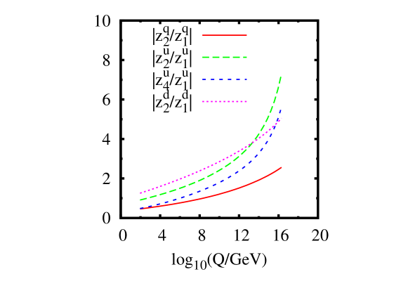
Figure 1: Selected MFV ratios $|z_{i}^{u,d,q}/z_{1}^{u,d,q}|$ in pure AMSB for $\tan\beta=10$ as a function of the renormalisation scale $Q$.

In Fig. 1 we plot some such selected ratios $|z_{i}^{u,d,q}/z_{1}^{u,d,q}|$ as a function of the renormalisation scale $Q$, which varies between $M_{Z}$ and $M_{{\scriptscriptstyle\rm GUT}}$. We see an increase with the scale in all the ratios, driven by the decrease of the flavour-blind contributions proportional to $z_{1}^{u,d,q}$ towards the GUT scale. The suppression of flavour violation with decreasing scale in the MSSM with general squark mixing has also been observed in Refs. [25, 19].

The observed behaviour of the flavour coefficients $z_{i}^{u,d,q}$ in AMSB is different from other common MFV MSSM models. While AMSB is nowhere flavour blind (except for, at small $\tan\beta$, in the limit ${\hat{\beta}}_{\lambda_{t}}\rightarrow 0$), both gauge mediation and (by construction) mSUGRA have flavour-diagonal sfermion masses at a certain high scale. In the latter models, the $z^{u,d,q}_{i>1}$ parameters are induced by renormalisation group evolution [26], and the ratios $|z_{i>1}^{u,d,q}/z_{1}^{u,d,q}|$ increase towards the weak scale. However, due to the automatic suppression by loop factors (times logs) and the enhancement of the $z_{1}^{u,d,q}$ terms by the gaugino contributions, the ratios $|z_{i>1}^{u,d,q}/z_{1}^{u,d,q}|$ remain small, in agreement with Eq. (41).

3.3 Solutions to the tachyonic slepton problem

An example of a scenario which fixes the tachyonic slepton problem without disturbing Eqs. (25a)–(25e) is provided by Ref. [21], where the MSSM is augmented by the addition to the superpotential of (non MFV) $R$-parity violating couplings of the form $\lambda_{ijk}L_{i}L_{j}\bar{E}_{k}$. These Yukawa couplings provide positive contributions to the slepton squared masses which can be sufficiently large, while leaving Eqs. (25a)–(25e) unaffected at the scale of the SUSY-breaking terms, $M_{{\scriptscriptstyle\rm SUSY}}$. Other solutions to the tachyonic slepton problem in which only the boundary conditions on the slepton masses themselves are modified will generally affect the squark masses as well, modifying their renormalisation group evolution below the scale at which the additional slepton masses are switched on. However, the slepton masses enter the one-loop $\beta$-functions for $m_{\tilde{Q}}^{2}$, $m_{\tilde{u}}^{2}$ and $m_{\tilde{d}}^{2}$ only via their contribution to the $U(1)_{Y}$ Fayet-Iliopoulos (FI) $S$-term [26] and consequently would have at most a small effect on the running for these quantities.

On the other hand if we adopt the popular mAMSB solution of Eq. (6) we must replace

$$m_{\tilde{Q}}^{2}\to m_{\tilde{Q}}^{2}+m_{0}^{2}\,\mathbf{1},\qquad m_{\tilde{u}}^{2}\to m_{\tilde{u}}^{2}+m_{0}^{2}\,\mathbf{1},\qquad m_{\tilde{d}}^{2}\to m_{\tilde{d}}^{2}+m_{0}^{2}\,\mathbf{1}$$ (49)

in Eqs. (25a)–(25c) and apply the theoretical boundary condition at the gauge unification scale $M_{{\scriptscriptstyle\rm GUT}}$. The MSSM renormalisation group equations, which deviate from the pure AMSB trajectory, must then be run down to the SUSY scale $M_{{\scriptscriptstyle\rm SUSY}}$ in order to determine the mass spectrum. Note that even a flavour-universal shift to the squark masses, such as the one in Eq. (49), affects the flavour-mixing mass parameters via the running between $M_{{\scriptscriptstyle\rm GUT}}$ and $M_{{\scriptscriptstyle\rm SUSY}}$. For instance, the beta function for $(m^{2}_{\tilde{Q}_{L}})_{ij}$ (where $i\neq j$) contains a piece [26] $(\beta_{m^{2}_{{\tilde{Q}}_{L}}})_{ij}=\sum_{l}(m^{2}_{{\tilde{Q}}_{L}})_{ii}V_{il}^{\dagger}({\hat{Y}}_{U})_{ll}^{2}V_{lj}+\ldots$, where ${\hat{Y}}_{U}$ is the diagonalised up-quark Yukawa matrix. Thus, a change to the flavour-universal piece of the squark mass matrix $(m^{2}_{{\tilde{Q}}_{L}})_{ii}$ induces a change in $(m^{2}_{{\tilde{Q}}_{L}})_{ij}$.

With the $U(1)$-based solution of Eq. (7) we should really distinguish the two alternatives we consider. With the $U(1)^{\prime}$ model (Table 1) we have

$$m_{\tilde{Q}}^{2}\to m_{\tilde{Q}}^{2}-\xi\,\frac{L}{3}.\mathbf{1},\ \ m_{\tilde{u}}^{2}\to m_{\tilde{u}}^{2}-\xi\left(e+\frac{2}{3}L\right).\mathbf{1},\ \ m_{\tilde{d}}^{2}\to m_{\tilde{d}}^{2}+\xi\left(e+\frac{4}{3}L\right).\mathbf{1}\,.$$ (50)

In this case the non-FI contributions to the masses retain RG invariance, in the sense that applying Eq. (50) at $M_{{\scriptscriptstyle\rm GUT}}$ with a given $(\xi e,\xi L)$ pair corresponds to the same physics as applying the same equation at $M_{{\scriptscriptstyle\rm SUSY}}$ with a different pair. For example, with $m_{3/2}=40~{}\hbox{TeV}$ and $\tan\beta=10$, and fixing for simplicity $\xi=1$ TeV² at both scales, the choice $(e,L)=(0.25,0)$ at $M_{{\scriptscriptstyle\rm GUT}}$ corresponds to $(e,L)\approx(0.06,0.09)$ at $M_{{\scriptscriptstyle\rm SUSY}}$. The reason this does not correspond simply to a renormalisation of $\xi$ is that, as well as such a renormalisation, a FI term associated with $U(1)_{Y}$ is generated when we run down from $M_{{\scriptscriptstyle\rm GUT}}$. This FI term can be absorbed into the existing one by redefining $L$ and $e$. For a detailed discussion see Section 4 and in particular Eq. (3.17) of Ref. [16]. The allowed region in the $(e,L)$ plane has been discussed in Ref. [14], see Fig. 1 of that reference. With $m_{3/2}=40~{}\hbox{TeV}$ and $\xi=1$ TeV², one needs $L\lower 2.0pt\hbox{$\,\buildrel{\scriptstyle>}\over{\scriptstyle\sim}\,$}0.03$ and $e\lower 2.0pt\hbox{$\,\buildrel{\scriptstyle>}\over{\scriptstyle\sim}\,$}0.04$ (at $M_{{\scriptscriptstyle\rm SUSY}}$) to avoid negative square masses for the slepton doublets and singlets, respectively, and it transpires one also needs $L+e\lower 2.0pt\hbox{$\,\buildrel{\scriptstyle<}\over{\scriptstyle\sim}\,$}0.17$ in order that the Higgs potential gives rise to the electroweak vacuum. Thus, values of $(e,L)$ of ${\cal O}(0.1)$ are viable.

With the alternative of $U(1)_{SU(5)}$ from Table 2 we have

$$m_{\tilde{Q}}^{2}\to m_{\tilde{Q}}^{2}+\xi e.\mathbf{1},\qquad m_{\tilde{u}}^{2}\to m_{\tilde{u}}^{2}+\xi e.\mathbf{1},\qquad m_{\tilde{d}}^{2}\to m_{\tilde{d}}^{2}+\xi L.\mathbf{1}\,,$$ (51)

but in this case the non-FI contributions to the masses are not RG invariant because the low energy theory has $U(1)_{SU(5)}$ anomalies, so we must again apply the theoretical boundary condition at $M_{{\scriptscriptstyle\rm GUT}}$ and run the MSSM RGEs down to the weak scale. As discussed in Ref. [16], there are lower limits on $L$ and $e$ comparable to those found in the $U(1)^{\prime}$ case, but also a dramatic difference in that increasing $(e,L)$ with $L\approx e$ does not lead to loss of the electroweak vacuum. The reason for this is that in this case the FI contributions to the square masses of both Higgses are negative. Of course, increasing $(e,L)$ scales up the squark and slepton masses, $|m^{2}_{H_{1,2}}|$ and hence the superpotential Higgs mass parameter $\mu$, thus increasing the fine tuning known as the little hierarchy problem.

In all three cases we anticipate that, because of the flavour-blind nature of the modification of the scalar masses, our expectation that flavour violation will be suppressed at low $\tan\beta$ will turn out to be true; it is clear, of course, that if we were to use a $U(1)$ with family-dependent charges in Eq. (50) or Eq. (51) we would compromise the MFV structure and inevitably face FCNC problems [10].

4 Predictions of Squark Flavour Violation

In order to quantify AMSB predictions for flavour violation, we use SOFTSUSY3.0 [27], which includes full three-family flavour mixing. We consider the range $m_{3/2}=40-140$ TeV, where the lightest supersymmetric particle mass is $m_{\chi_{1}^{0}}\sim 130-520$ GeV and the gluino mass is $m_{\tilde{g}}=800-3100$ GeV, in the interesting range for LHC SUSY discovery [28]. There are no direct SUSY-search constraints conflicting with $3<\tan\beta<42$ and 40 TeV $<m_{3/2}<$ 140 TeV, therefore this is the range taken. See Appendix A for further details on input parameters and the calculation.

4.1 Flavour-changing squark mass insertions in AMSB

We now calculate the flavour-changing squark mass insertions in AMSB. First, the Lagrangian parameters are transformed to the super-CKM basis described in Section 2.2, by rotating the one-loop corrected squark mass matrices by the same mixing matrix required to diagonalise the quark Yukawa matrices at $M_{{\scriptscriptstyle\rm SUSY}}$. We may then define the usual flavour-violating mass-insertion parameters $\delta^{q}$ from the entries of the 6$\times$6 squark mass matrices ${\mathcal{M}}_{\tilde{u}}^{2}$ and ${\mathcal{M}}_{\tilde{d}}^{2}$ defined in Eqs. (17) and (21)

$$(\delta^{q}_{ij})_{LL} = \frac{({\mathcal{M}}_{\tilde{q}}^{2})_{ij}}{\sqrt{({\mathcal{M}}_{\tilde{q}}^{2})_{ii}({\mathcal{M}}_{\tilde{q}}^{2})_{jj}}},\quad(\delta^{q}_{ij})_{RR}=\frac{({\mathcal{M}}_{\tilde{q}}^{2})_{i+3\ j+3}}{\sqrt{({\mathcal{M}}_{\tilde{q}}^{2})_{i+3\ i+3}({\mathcal{M}}_{\tilde{q}}^{2})_{j+3\ j+3}}},$$

$$(\delta^{q}_{ij})_{LR} = \frac{({\mathcal{M}}_{\tilde{q}}^{2})_{i\ j+3}}{\sqrt{({\mathcal{M}}_{\tilde{q}}^{2})_{ii}({\mathcal{M}}_{\tilde{q}}^{2})_{j+3\ j+3}}},$$ (52)

with $i,j\in\{1,2,3\}$ and $q=u,d$. In this section we shall compare the AMSB prediction of $\delta^{q}$ originating from Eqs. (25a)–(25e) with the empirical bounds from Ref. [29].

Figure 2: Magnitudes of selected flavour-violating mass insertions $\delta^{q}$ in AMSB as functions of $\tan\beta$. When two curves are visible for the same $\delta^{q}$, the upper curve is for $m_{3/2}=40$ TeV and the lower curve is for $m_{3/2}=140$ TeV.

In Fig. 2a we show the $\tan\beta$ dependence of the absolute values of the flavour-violating up-squark mass insertions $(\delta^{u}_{12})_{LL}\,,~{}{(\delta^{u}_{13})_{LL}}\,,~{}(\delta^{u}_{23})_{LL}$ and $(\delta^{u}_{23})_{LR}$ in the “pure” AMSB scenario, where we assume that Eqs. (25a)–(25c) are unaffected by the mechanism that fixes the tachyonic slepton problem; while in Fig. 2b we show the corresponding results for the down-squark sector. The two curves for $(\delta^{u,d}_{23})_{LR}$ visible in each plot correspond to $m_{3/2}=40$ GeV (upper curve) and $m_{3/2}=140$ GeV (lower curve), respectively. Indeed, Eqs. (17), (21), (35), (30) and (52) imply that $(\delta^{u,d}_{ij})_{LR}$ are inversely proportional to $m_{3/2}$ for $i\neq j$, whence the significant, ${\mathcal{O}}(100\%)$ dependence upon the SUSY-breaking scale. On the other hand, Eqs. (25a)–(25c) combined with Eq. (52) imply that there is no dependence of $(\delta^{u,d}_{ij})_{LL,RR}$ on $m_{3/2}$ [aside from logarithmic corrections coming from scale dependence of the right-hand side of Eqs. (25a)–(25c)]. In Figs. 2a and 2b the curves for $(\delta^{u,d}_{ij})_{LL}$ that correspond to the two different values of $m_{3/2}$ are practically overlaid. We also see from the figures that the mass insertions in the up-squark sector show a significant dependence on $\tan\beta$, while the dependence in the down-squark sector is much less pronounced. The reason for this is quite simple. We can see from Eqs. (26) and (34) that the down-squark sector off-diagonal elements are more sensitive to $\lambda_{t}$ and the up-squark off-diagonal elements are more sensitive to $\lambda_{b}$; but as $\tan\beta$ increases from $5$ to $40$, $\sin\beta$ (and hence $\lambda_{t}$) scarcely changes but $\cos\beta$ (and hence $\lambda_{b}$) changes by a factor of 12.

In our solutions to the slepton mass problem, the additional contributions in Eqs. (49), (50) and (51) affect only the diagonal terms of the squark mass matrices at the scale at which they are applied (i.e., $M_{{\scriptscriptstyle\rm SUSY}}$ for the $U(1)^{\prime}$ solution and $M_{{\scriptscriptstyle\rm GUT}}$ for mAMSB and $U(1)_{SU(5)}$). For a model such as the $U(1)^{\prime}$ solution in Eq. (50), which preserves the RG invariance of the expressions for squark soft SUSY-breaking terms, the change in the magnitudes of the $\delta^{q}$ parameters with respect to the pure AMSB case can be directly estimated by the effect of the slepton mass fix on the diagonal squark mass parameters. Thus, denoting $x_{ij}^{q}\equiv\sqrt{({\mathcal{M}}_{\tilde{q}}^{2})_{ii}({\mathcal{M}}_{\tilde{q}}^{2})_{jj}}$ ,

$$\frac{\Delta|(\delta_{ij}^{q})_{XY}|}{|(\delta_{ij}^{q})_{XY}|}\approx-\frac{\Delta x^{q}_{ij}}{x_{ij}^{q}},$$ (53)

with $q=u,d$. Interestingly, in the $U(1)$-inspired solutions the shifts $\Delta x^{q}_{ij}$ enter the up and down singlet and doublet squark masses in a non-universal way, hence the relative size of $\delta^{q}_{LR}$ versus $\delta^{q}_{LL}$ can be modified at this level.

The experimental upper bounds upon the $\delta^{q}$ parameters depend upon the squark masses and the ratio of the gluino mass to the squark masses. In order to obtain a rough estimate, we have fitted the constraints in Ref. [29] with a parabola to determine the dependence upon the gluino/squark mass ratio (whereas there is a simple scaling relation with the squark mass itself). We detail some of the larger $\delta^{q}$ parameters in Appendix A for four AMSB variants. However, the bottom line is that all $\delta^{q}$ are easily within their experimental bounds, regardless of which tachyonic slepton fix is taken. AMSB is far from being ruled out on the basis of these naive empirical flavour constraints, the closest to the bound being $(\delta_{13}^{d})_{LL}\sim\mathcal{O}(10^{-3})$, which has a bound of $(\delta_{13}^{d})_{LL}<0.16$ [29]. However, the mass insertions that mix the second and third generations can affect the prediction of the branching ratios for rare $B$ decays such as $B\rightarrow X_{s}\gamma$ and $B_{s}\rightarrow\mu\mu$, by mediating the $b\rightarrow s$ transition in loops involving squarks. In Sections 4.3 and 4.4 we will examine these important physical observables, whose uncertainties have been vastly reduced since Ref. [29].

4.2 AMSB prediction for the charged Higgs mass

The Higgs sector of the MSSM (for a review see, e.g., Ref. [30]) contains two CP-even neutral scalars $h$ and $H$, a CP-odd neutral scalar $A$ and a charged scalar $H^{\pm}$. One of the CP-even scalars as well as $A$ and $H^{\pm}$ have couplings to the down-type fermions that are enhanced by $\tan\beta$ with respect to the couplings of the SM Higgs boson. Thus, even in SUSY-breaking scenarios such as AMSB in which the super particles are typically rather heavy, there can be sizeable contributions to rare $B$ decays from diagrams involving the non-standard Higgs bosons, if the latter are light and $\tan\beta$ is large [31].

For moderate-to-large $\tan\beta$ the non-standard CP-even scalar is close in mass to the CP-odd scalar, whose mass is determined by $m_{A}^{2}=2\,B\,/\sin 2\beta$ at tree level. The masses of the CP-odd and charged scalars are in turn related at tree level by $m_{H^{\pm}}^{2}=m_{A}^{2}+m_{W}^{2}$. It is therefore useful to investigate the AMSB prediction for the charged Higgs boson mass $m_{H^{\pm}}$, bearing in mind that we determine the soft SUSY-breaking Higgs mass parameter $B$ by minimisation of the scalar potential. Inserting the pure AMSB expressions [3] for $m_{H_{1}}^{2}$ and $m_{H_{2}}^{2}$ in the tree-level formula for $m^{2}_{H^{\pm}}$ (see e.g. Ref. [32]), and neglecting contributions controlled by all Yukawa couplings other than $\lambda_{t}$ and $\lambda_{b}$, we obtain, in the large-$\tan\beta$ limit,

$$\frac{(16\pi^{2})^{2}}{m_{3/2}^{2}}~{}m_{H^{\pm}}^{2}~{}\approx~{}K\,-\,\left(3{\overline{\lambda}}_{b}^{2}\,C_{b}-36\,{\overline{\lambda}}_{b}^{4}\right)\,\tan^{2}\beta\,+\,18\,{\overline{\lambda}}_{b}^{4}\,\tan^{4}\beta,$$ (54)

where $K$ is positive and does not depend on $\tan\beta$ at tree level, $C_{b}$ is defined in Eq. (33b) and ${\bar{\lambda}}_{b}\equiv\lambda_{b}\,\cos\beta$. Since at tree level ${\bar{\lambda}}_{b}=\sqrt{2}\,m_{b}/v$, the coefficient of $\tan^{2}\beta$ is negative and Eq. (54) predicts a minimum for $m_{H^{\pm}}$ at a certain value of $\tan\beta$. However, for an accurate prediction of the position of the minimum we must take into account the $\tan\beta$-enhanced threshold corrections [33] to the relation between the bottom mass and the bottom Yukawa coupling, as well as the radiative corrections to the tree-level formula for $m^{2}_{H^{\pm}}$.

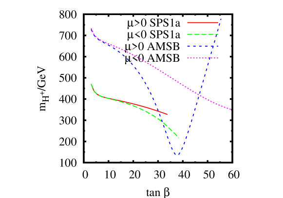
Figure 3: The charged Higgs boson mass as a function of $\tan\beta$ in mSUGRA model SPS1a and pure AMSB with $m_{3/2}=40$ TeV and either sign of $\mu$.

In Fig. 3 we show the full numerical dependence on $\tan\beta$ of $m_{H^{\pm}}$, as computed by SOFTSUSY for “pure” AMSB conditions, with $m_{3/2}=40$ TeV and either sign of $\mu$ (the $\mu>0$ curve terminates because the electroweak minimum of the Higgs potential becomes unstable). The marked difference between the curves corresponding to the two signs of $\mu$ is due to the fact that the $\tan\beta$-enhanced threshold corrections, whose effect depends on the sign of the product $m_{\tilde{g}}\,\mu$, enhance ${\bar{\lambda}}_{b}$ for $\mu>0$ and suppress it for $\mu<0$. In the former case the position of the minimum in $m_{H^{\pm}}$ is shifted towards smaller values of $\tan\beta$, while in the latter we see no stationary point up to $\tan\beta=60$. For comparison we also show $m_{H^{\pm}}$ as a function of $\tan\beta$ for the SPS1a mSUGRA point [34]; the dependence on $\tan\beta$ is much less marked. The curves end when the stau becomes tachyonic, signalling an inappropriate scalar potential minimum.

4.3 $B\rightarrow X_{s}\gamma$ constraints

Flavour-changing neutral current processes are loop suppressed in the SM as well as in the MSSM. In the SM the $b\rightarrow s\gamma$ transition is mediated at one loop by diagrams involving $W$ boson and up-type quarks. Additional one-loop contributions arise in the MSSM from diagrams involving a charged Higgs boson and up-type quarks, a chargino and up-type squarks and, in the presence of flavour violation in the squark sector, a gluino and down-type squarks. The contributions of diagrams with neutralinos and down-type squarks are suppressed with respect to the gluino loops by the smaller gauge coupling and by an accidental cancellation in the magnetic-chromomagnetic mixing.

The current experimental value of the branching ratio for the $B\rightarrow X_{s}\gamma$ decay is [35]

$${\rm BR}(B\rightarrow X_{s}\gamma)_{\rm exp}=(3.52\pm 0.23\pm 0.09)\times 10^{-4}~{},$$ (55)

for a photon energy $E_{\gamma}>1.6$ GeV. The corresponding next-to-next-to leading order (NNLO) SM prediction that was published two years ago reads [36]

$${\rm BR}(B\rightarrow X_{s}\gamma)_{\rm\,SM}=(3.15\pm 0.23)\times 10^{-4}~{},$$ (56)

and a recent update [37] of the calculation of the normalisation factor for the branching ratio results in a modest enhancement to $(3.28\pm 0.25)\times 10^{-4}$ (see also Ref. [38]). In both cases, the error on the theoretical prediction for the branching ratio is around 7%. Inflating the theoretical error to 10% we accommodate – rather conservatively – for the additional uncertainty arising from the calculation of the SUSY contributions to the decay. Thus, at 95$\%$ C.L., we may require $2.70\times 10^{-4}<{\rm BR}(B\rightarrow X_{s}\gamma)<4.34\times 10^{-4}$.

We use the public computer program SusyBSG 1.2 [39] to obtain a next-to-leading order (NLO) prediction of ${\rm BR}(B\rightarrow X_{s}\gamma)$ in the MSSM. The program implements the results of Ref. [40] for the two-loop gluon contributions to the Wilson coefficients of the magnetic and chromomagnetic operators relevant to the $b\rightarrow s\gamma$ transition, and the full results of Ref. [41] for the two-loop gluino contributions (accounting also for the $\tan\beta$-enhanced charged-Higgs contributions first discussed in Ref. [42]). While the two-loop contributions are computed in the approximation of neglecting flavour mixing in the squark sector, the computation of the one-loop contributions to the Wilson coefficients takes into account the full flavour structure of the squark mass matrices. The relation between the Wilson coefficients and ${\rm BR}(B\rightarrow X_{s}\gamma)$ is computed at NLO along the lines of Ref. [43], taking into account also the recent results of Ref. [37]. The free renormalisation scales of the NLO calculation are adjusted in such a way as to mimic the NNLO contributions that are not present in the calculation, reproducing the central value of the SM prediction of the branching ratio given in Ref. [37].

Figure 4: Constraints on the AMSB parameter space from the rare decay $B\rightarrow X_{s}\gamma$. (a) ${\rm BR}(B\rightarrow X_{s}\gamma)$ as a function of $\tan\beta$ for $m_{3/2}=40$ TeV and both signs of $\mu$. (b) ${\rm BR}(B\rightarrow X_{s}\gamma)$ displayed as the background colour for $\mu>0$ in the $\tan\beta-m_{3/2}$ plane. For the explanation of the various curves in both panels see the text.

Fig. 4a displays ${\rm BR}(B\rightarrow X_{s}\gamma)$ as a function of $\tan\beta$, for $m_{3/2}=40$ TeV and either sign of $\mu$, assuming that the squarks do not deviate from the pure AMSB trajectory. The red (solid) curves include all effects in the calculation of the Wilson coefficients, while the blue (dotted) curves ignore flavour-mixing effects in the squark masses. The green shaded region represents the 95% C.L. limits on the branching ratio. The difference between the curves corresponding to the two signs of $\mu$ is due to the combination of two factors. First of all, as discussed above, the $\tan\beta$-enhanced threshold corrections to the relation between the bottom mass and the bottom Yukawa coupling result in a much lighter charged Higgs boson – thus an enhanced contribution to the Wilson coefficients – for $\mu>0$ (the peak in the branching ratio around $\tan\beta\sim 37$ corresponds indeed to the minimum in $m_{H^{\pm}}$ shown in Fig. 3). In addition, the contributions to the Wilson coefficients from diagrams involving the top quark and the charged Higgs boson and those from diagrams involving squarks and charginos – the latter depending on the sign of the product $A_{t}\,\mu$, where $A_{t}\equiv(\widehat{T}_{U})_{33}/\lambda_{t}$ – interfere constructively for $\mu>0$ and destructively for $\mu<0$. We remark that in the traditional mSUGRA scenario, in which $m_{\tilde{g}}$ (and, in most cases, $A_{t}$) have opposite sign with respect to the prediction of AMSB, the dependence of ${\rm BR}(B\rightarrow X_{s}\gamma)$ on the sign of $\mu$ is reversed [42].

The flavour-changing mass insertions $(\delta^{d}_{23})_{LL}$ and $(\delta^{d}_{23})_{LR}$ mediate the $b\rightarrow s\gamma$ transition in one-loop diagrams involving gluinos and down-type squarks. In addition, $(\delta^{u}_{23})_{LL}$ can contribute a sizeable amount to one-loop diagrams involving charginos and up-type squarks (the smallness of the flavour-changing mass insertion being compensated by the fact that the wino-strange-scharm vertex is not Cabibbo-suppressed). From the comparison between the red (solid) and blue (dotted) curves in Fig. 4a we see that the flavour-violating effects have a comparatively large effect (up to 10$\%$) on the predicted value of ${\rm BR}(B\rightarrow X_{s}\gamma)$ for large $\tan\beta$. We also see that, had we not included squark flavour-violating effects in the calculation of ${\rm BR}(B\rightarrow X_{s}\gamma)$, we would have deduced that for $\mu>0$ the empirical limit leads to $\tan\beta=15$, which is too weak by around 10$\%$. For $\mu<0$, neglecting squark flavour violation would have resulted on the $\tan\beta$ bound being roughly 30% too high.

Fig. 4b displays ${\rm BR}(B\rightarrow X_{s}\gamma)$ as the background colour in the $\tan\beta-m_{3/2}$ plane, for $\mu>0$. The yellow (dot-dashed) contour on the left delimits the regions ruled out by the LEP2 Higgs-mass constraints. The red (dotted) contour on the right is the bound on the $\tan\beta-m_{3/2}$ plane obtained by applying the 95% C.L. experimental upper bound on the branching ratio. The green (dashed) rightmost contour is the bound that would be obtained if the squark flavour mixing effects were ignored. For a given value of $m_{3/2}$, the upper limit on ${\rm BR}(B\rightarrow X_{s}\gamma)$ effectively provides an upper bound on the parameter $\tan\beta$, because the SUSY contribution is enhanced for large $\tan\beta$. We see that the strictest bound is $\tan\beta<13$ for $m_{3/2}=40$ TeV but this relaxes to $\tan\beta<35$ for $m_{3/2}=140$ TeV, where heavier charged Higgs boson and heavier sparticles provide a suppression of the SUSY contribution to ${\rm BR}(B\rightarrow X_{s}\gamma)$.

4.4 Implications for $B_{s}\to\mu\mu$ and future impact

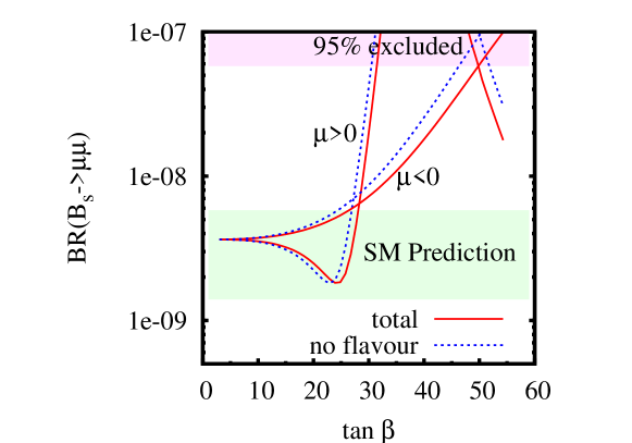
Figure 5: BR($B_{s}\rightarrow\mu\mu$) in pure AMSB with (“total”) or without (“no flavour”) squark flavour changing contributions to down-squark gluino loops for $m_{3/2}=40$ TeV and either sign of $\mu$. Also shown is the SM prediction and the current experimental upper bound [45].

The supersymmetric Higgs spectrum has a significant impact on the rare leptonic decay $B_{s}\rightarrow\mu\mu$. Specifically, the decay amplitude receives $\tan\beta$-enhanced contributions proportional to $1/m_{A}^{2}$ from neutral-Higgs exchange [46, 47]. In our determination of the MSSM prediction for BR$(B_{s}\to\mu\mu)$ we implemented the results of Ref. [47] for the subset of one-loop contributions involving up-type squarks and charginos that are enhanced by $\tan^{3}\beta$, as well as the results of Ref. [48] for the one-loop contributions involving down-type squarks and gluinos. The latter are relevant in the presence of flavour mixing in the down squark sector; the dominant contribution in AMSB stems from $(\delta^{d}_{23})_{LL}$, which, at $10^{-2}$, is one of the largest mass insertions (see Fig. 2). Finally, for the treatment of the $\tan\beta$-enhanced, higher-order contributions that originate in the corrections to the relation between the down-quark masses and Yukawa couplings we followed Ref.[49] (see also Ref. [50]). We checked the relevant part of our results against micrOMEGAS 2.1 [51], which however does not include the effect of flavour mixing in the squark sector.

Fig. 5 shows BR$(B_{s}\to\mu\mu)$ in pure AMSB as a function of $\tan\beta$, for $m_{3/2}=40$ TeV and either sign of $\mu$. The red (solid) lines represent the total result, while the blue (dotted) lines neglect the effect of flavour mixing in the squark sector. For the SM branching ratio we obtain BR$(B_{s}\rightarrow\mu\mu)_{\rm SM}=(3.6\pm 0.9)\times 10^{-9}$, with the uncertainty dominated by the one of the $B_{s}$-meson decay constant $f_{B_{s}}=0.24\pm 0.03$ GeV [52]. For $\mu>0$ the effect of the dip in $m_{A}$ (recall that $m_{A}\approx m_{H^{\pm}}$) around $\tan\beta\sim 35-40$ is clearly visible in the steep rise of the $B_{s}\rightarrow\mu\mu$ branching ratio. For $\mu<0$ the $\tan\beta$-enhanced corrections to the Higgs-quark-quark coupling cause a milder increase with $\tan\beta$ (recall that in AMSB the relative sign between $\mu$ and the gluino mass is opposite to the one in mSUGRA). Our analysis also shows that – contrary to what happens in ${\rm BR}(B\rightarrow X_{s}\gamma)$ – in BR$(B_{s}\rightarrow\mu\mu)$ the inclusion of squark flavour mixing reduces the deviation from the SM at large $\tan\beta$. Here, the relative sign between the chargino and gluino contributions is ${\rm sign}(A_{t}\,m_{\tilde{g}}\,(\delta^{d}_{23})_{LL})$, which is negative in AMSB. The effect of the gluino contribution is important and accounts for changes up to a factor of two in the branching ratio. We also show in Fig. 5 the experimental 95% C.L. upper bound BR$(B_{s}\rightarrow\mu\mu)<58\times 10^{-9}$ [45], which is an order of magnitude above the SM value. Fig. 5 shows that current $B_{s}\rightarrow\mu\mu$ data is not as constraining as the $B\rightarrow X_{s}\gamma$ branching ratio shown in Fig. 4a, but if the experimental limit on BR$(B_{s}\rightarrow\mu\mu)$ approaches the Standard Model prediction in the future, for the $\mu<0$ branch, $B_{s}\rightarrow\mu\mu$ will become more constraining than $B\rightarrow X_{s}\gamma$.

Figure 6: BR($B_{s}\rightarrow\mu\mu$) in pure AMSB displayed as the background colour in the $\tan\beta-m_{3/2}$ plane, for (a) $\mu<0$ and (b) $\mu>0$. For the explanation of the various curves in both panels see the text.

In Fig. 6 we show BR($B_{s}\rightarrow\mu\mu$) in pure AMSB as the background colour in the $\tan\beta-m_{3/2}$ plane, for (a) $\mu<0$ and (b) $\mu>0$. Constraints from a hypothetical measurement of the branching ratio at $1\times 10^{-8}$ (solid line) and $5\times 10^{-9}$ (dashed line) are given for illustration. Superimposed on each panel are the boundaries of the allowed region, which are as in Fig. 4b: the yellow (dash-dotted) line delimits the parameter space allowed by the LEP2 Higgs search, whereas the magenta (dotted) line marks the border of parameter space allowed by $B\rightarrow X_{s}\gamma$. Hence, for $\mu>0$, the $B\rightarrow X_{s}\gamma$ constraint rules out the possibility of a large $B_{s}\to\mu\mu$ enhancement at large $\tan\beta$. Note that if we were to include also the constraints on the muon anomalous magnetic moment, which requires a positive $\mu$ term (see Section 4.6), we would predict the $B_{s}\to\mu\mu$ branching ratio to not exceed its SM value.

With improved data the rare leptonic mode will hence become increasingly important. Searches for $B_{s}\to\mu\mu$ are ongoing at the Tevatron collider and will commence at the LHC. The LHCb experiment will be able to exclude or discover new physics in $B_{s}\to\mu\mu$ after one year, while ATLAS and CMS will be able to do so after three years of operation [53].

4.5 Charged Higgs effects in $B\to\tau\nu$

Substantial effects in the leptonic $B\to\tau\nu$ decays are possible from charged Higgs exchange at large $\tan\beta$ [54]. It is customary to study the branching ratio normalised to the SM one, which yields a simple expression [55]

$$R_{\tau\nu}\equiv\frac{\mbox{BR}(B\to\tau\nu)}{\mbox{BR}(B\to\tau\nu)_{\rm SM}}=\left(1-\frac{m_{B}^{2}}{m_{H^{\pm}}^{2}}\frac{\tan^{2}\beta}{1+\epsilon_{g}\tan\beta}\right)^{2}.$$ (57)

Here, $m_{B}$ denotes the mass of the $B$ meson and $\epsilon_{g}$ is the gluino-induced correction to the relation between the mass of the bottom quark and its Yukawa coupling.

In Fig. 7 we show $R_{\tau\nu}$ in AMSB for $m_{3/2}=40$ TeV. For $\mu>0$ the sharp peak around $\tan\beta\sim 37$ from the $m_{H^{\pm}}$ dip is clearly visible. Using the stronger constraint on $\tan\beta$ from ${\rm BR}(B\rightarrow X_{s}\gamma)$, we predict $0.83(0.96)<R_{\tau\nu}\leq 1$ for $\mu>0\,(\mu<0)$. Thus, $R_{\tau\nu}$ is constrained to be below unity within AMSB, which is natural in large-$\tan\beta$ MFV scenarios [55].

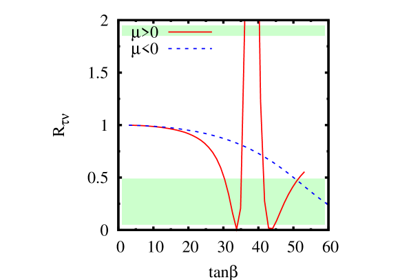
Figure 7: The ratio $R_{\tau\nu}$ Eq. (57) in pure AMSB for $m_{3/2}=40$ TeV and either sign of $\mu$. The green regions are disfavoured at the 2$\sigma$ level.

The branching ratio has been measured at the $B$-factories by Belle and BaBar [56] $\mbox{BR}(B\to\tau\nu)=(1.51\pm 0.33)\times 10^{-4}$ with the average provided by [35]. With $|V_{ub}|=(3.95\pm 0.35)\times 10^{-3}$ [57] and the $B$-meson decay constant $f_{B}=0.216\pm 0.022$ GeV [58] the SM prediction for the branching ratio is given as

$$\mbox{BR}(B\to\tau\nu)_{\rm SM}=1.29\times 10^{-4}\left(\frac{|V_{ub}|}{3.95\cdot 10^{-3}}\right)^{2}\left(\frac{f_{B}}{0.216\,\mbox{GeV}}\right)^{2},$$ (58)

with a net uncertainty of 19%. For the ratio between experimental result and SM prediction we obtain $R_{\tau\nu}^{\rm exp}=1.17\pm 0.34$, where we added the uncertainties in quadrature.

We remark that the value of $|V_{ub}|$ used here results from combining data on inclusive and exclusive $b\to u$ decays. Currently, the individual determinations of $|V_{ub}|$ are not in perfect agreement with each other, i.e., the exclusive modes prefer a lower value than the inclusive ones. Recent lattice computations [59] also give lower values for $f_{B}$ and hence favour a somewhat larger $R_{\tau\nu}^{\rm exp}$ of 1.44$\pm$0.38, which is harder to accommodate within SUSY. Furthermore, the experimental situation for $B\to\tau\nu$ is also still improving; at a high-luminosity $e^{+}e^{-}$ machine [60], a measurement of the branching ratio could perhaps be made with an uncertainty of 10% (for 10 $\mbox{ab}^{-1}$). Given the situation, at present we cannot draw definite conclusions for AMSB from $B\to\tau\nu$, but note that this mode has the potential to become important in the future.

4.6 Comment on $(g-2)_{\mu}$

In the AMSB context, having discussed ${\rm BR}(B\rightarrow X_{s}\gamma)$, it behoves us to comment on the supersymmetric contribution to the muon anomalous magnetic moment $\delta a_{\mu}$. Relying on $e^{+}e^{-}$ data for some of the hadronic components, one finds [61] that

$$\delta a_{\mu}\equiv\delta\frac{(g-2)_{\mu}}{2}=(29.5\pm 8.8)\times 10^{-10}$$ (59)

is the discrepancy between the empirical value and the Standard Model (SM) prediction. The one-loop gaugino contribution to this is given at large $\tan\beta$ by [5, 62, 63]

$$a_{\mu}^{{SUSY}}\approx\frac{m_{\mu}^{2}\mu\tan\beta}{16\pi^{2}}\left(g_{1}^{2}M_{1}F_{1}+g_{2}^{2}M_{2}F_{2}\right),$$ (60)

where $F_{1,2}$ are positive definite functions of the slepton, chargino and neutralino masses, behaving like $1/M_{{\scriptscriptstyle\rm SUSY}}^{4}$ in the approximation that the relevant sparticles are degenerate in mass. Thus for $M_{1},M_{2}>0$, as is the case in AMSB, a supersymmetric explanation of the discrepancy between the SM and experiment favours $\mu>0$. But we see from Fig. 4 that it is the $\mu>0$ case that is restricted by ${\rm BR}(B\rightarrow X_{s}\gamma)$. So as remarked, e.g., in Ref. [64], this creates a potential difficulty for explaining the discrepancy between theory and experiment for $a_{\mu}$ using AMSB.

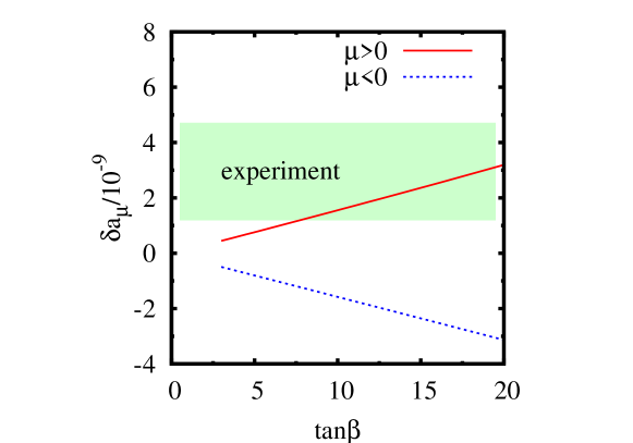
Figure 8: Supersymmetric contribution to the anomalous magnetic moment of the muon in $U(1)^{\prime}$ AMSB, for $m_{3/2}=40$ TeV and either sign of $\mu$. The experimental constraint listed is at the 95$\%$ confidence level.

Since $F_{1,2}$ depend upon the slepton masses, the prediction of $\delta a_{\mu}$ in AMSB models depends to a large extent upon the slepton mass fix that is employed. In Fig. 8, we show such a prediction for the $U(1)^{\prime}$ fix. We take the one-loop results for $\delta a_{\mu}$ from Ref. [64], supplementing them with the two-loop leading-log QED correction from Ref. [65] and the $\tan\beta$-enhanced contribution from Ref. [63]. In the figure, it is clear how the $\mu>0$ prediction in the red (solid) line fits the empirical 95$\%$ confidence level value of $\delta a_{\mu}$ for $\tan\beta>8$. Comparison with Fig. 4a then shows a region $8<\tan\beta<14$ which is compatible with both $\delta a_{\mu}$ and $B\rightarrow X_{s}\gamma$ constraints.

5 Conclusions

We have investigated flavour violation in the squark sector in various versions of AMSB; squark mixings are always readily calculable because of the simple and constrained nature of supersymmetry breaking terms in anomaly mediation. The resulting supersymmetric contributions to flavour-changing processes are CKM-induced and hence small. The model thus is consistent with all observations of quark flavour change. Quark electric dipole moment constraints imply fairly strict bounds on the imaginary phases on $|{\rm Im}(\delta^{u,d}_{11})_{LR}|<{\mathcal{O}}(10^{-6})$  [29], but these are easily satisfied due to the real coefficients multiplying the Yukawa matrices in Eqs. (25d) and (25e).

At present, the branching ratio $B\rightarrow X_{s}\gamma$ provides the most stringent constraint on the model, and receives non-negligible supersymmetric flavour corrections, affecting upper bounds on $\tan\beta$. As we demonstrated, in the future, $B_{s}\to\mu\mu$ and $B\to\tau\nu$ decays will provide complementary constraints. We have also shown explicitly that there are regions of AMSB parameter space that can accommodate the measurements of the $B\rightarrow X_{s}\gamma$ branching ratio as well as the anomalous magnetic moment of the muon, depending on the precise model for fixing the tachyonic slepton problem. Indeed, a recent $\chi^{2}$ analysis of electroweak and baryon precision observables favoured mAMSB over mSUGRA and minimal gauge mediation [66]; note, however, that this analysis neglected inter-generational squark mixing effects.

Predictivity in the flavour sector makes the AMSB scenario an attractive alternative to mSUGRA, whose family-universal pattern of SUSY-breaking sfermion masses is at best approximate. It is not immediately clear without further model building how the flavour off-diagonal pieces of the sfermion mass squared matrices are suppressed in order to give the mSUGRA pattern. Moreover, AMSB soft SUSY-breaking terms are always present; the issue is whether, as we have assumed here, they represent the dominant contributions to supersymmetry breaking.

Of course AMSB is not without its problems; the origin of the Higgs $\mu$ term (and of the associated soft SUSY-breaking $B$ term) is model dependent, and in minimal versions the lightest supersymmetric particle is the neutral wino, which represents a problematic dark matter candidate. These difficulties are not insuperable, however (for one approach see Ref. [15]). We believe that it is perhaps time for AMSB to be afforded status comparable to mSUGRA in modelling our expectations (or hopes) for what will be seen at the LHC. In any case, the two models should be easily discriminated in the event of a supersymmetric signal at the LHC [28] due to their widely different predicted patterns of supersymmetric masses and associated signals.

We close with some general remarks on quark flavour physics. The flavour changing signals of AMSB are MFV in character: they feature CKM-induced CP asymmetries, suppressed wrong-chirality contributions and CKM relations between $b\to s$ and $b\to d$ processes [67]. Because these models contain only a minimal amount of flavour and CP violation, their experimental separation from the SM background needs precise measurements, feasible perhaps at super flavour factories [53, 60].

Appendix A Numerical Detail of Squark Flavour Violation

In this appendix we collate the input parameters and detail of the numerical calculation of the $\delta^{q}$ parameters as implemented in SOFTSUSY 3.0. The sparticle pole masses receive one-loop corrections to the flavour conserving pieces, and family mixing is included at the tree level. SOFTSUSY solves the MSSM renormalisation group equations to two-loop order consistent with this theoretical boundary condition and SM data. Fermion masses and gauge couplings are obtained at $M_{Z}$ using an effective field theory of 3-loop QCD $\times$ 1-loop QED below $M_{Z}$. Our default SM data set contains the $\rm{\overline{MS}}$ quark masses $m_{u}(2\mbox{~{}GeV})=2.4$ MeV, $m_{d}(2\mbox{~{}GeV})=4.75$ MeV, $m_{s}(2\mbox{~{}GeV})=104$ MeV, $m_{c}(m_{c})=1.27$ GeV, $m_{b}(m_{b})=4.23$ GeV [57]. The top quark mass input is the pole mass, $m_{t}=172.4$ GeV [68], and the strong gauge coupling in the $\rm{\overline{MS}}$ scheme $\alpha_{s}(M_{Z})=0.1176$ [57]. We fix $M_{Z}=91.1876$ GeV to its central value [57], as well as the Fermi constant from muon decays, $G_{\mu}=1.16637\times 10^{-5}$ GeV^-2. $\alpha(M_{Z})=1/127.925$ is fixed to be the $\rm{\overline{MS}}$ value of the QED gauge coupling. The CKM mixing is parameterised by the Wolfenstein parameters at their central empirical values [57]: $\lambda=0.2258$, $A=0.814$, $\bar{\eta}=0.349$ and $\bar{\rho}=0.135$.

	$U(1)^{\prime}$	pure	$\Re$pure	mAMSB	$U(1)_{SU(5)}$
$~{}~{}m_{{\tilde{u}}_{L}}$/GeV	821	817	817	853	877
$~{}~{}m_{{\tilde{u}}_{R}}$/GeV	826	822	822	857	881
$~{}~{}m_{{\tilde{d}}_{L}}$/GeV	825	820	820	856	880
$~{}~{}m_{{\tilde{d}}_{R}}$/GeV	832	828	828	864	887
$~{}~{}m_{{\tilde{t}}_{L}}$/GeV	733	729	729	754	793
$~{}~{}m_{{\tilde{t}}_{R}}$/GeV	636	632	632	645	703
$~{}~{}m_{{\tilde{b}}_{L}}$/GeV	722	718	718	743	782
$~{}~{}m_{{\tilde{b}}_{R}}$/GeV	821	816	816	852	876
$(\delta^{u}_{13})_{LL}/10^{-5}$	$-2.0+5.2i$	$-2.0+5.3i$	$-5.6$	$-5.7$	$-5.1$
$(\delta^{u}_{23})_{LL}/10^{-4}$	$-6.4+0.0i$	$-6.6+0.0i$	$-6.5$	$-6.6$	$-5.9$
$(\delta^{u}_{23})_{LR}/10^{-5}$	$-6.5-0.0i$	$-6.7+0.0i$	$-6.7$	$-6.4$	$-5.8$
$(\delta^{d}_{12})_{LL}/10^{-5}$	$~{}~{}\,7.4+3.1i$	$~{}~{}\,7.4+3.1i$	$~{}~{}\,5.4$	$~{}~{}\,5.7$	$~{}~{}\,4.8$
$(\delta^{d}_{13})_{LL}/10^{-3}$	$-2.0+0.8i$	$-2.0-0.8i$	$-1.5$	$-1.6$	$-1.3$
$(\delta^{d}_{23})_{LL}/10^{-2}$	$~{}1.0+0.0i$	$~{}~{}\,1.0+0.0i$	$~{}~{}\,1.0$	$~{}~{}\,1.0$	$~{}~{}\,0.9$
$(\delta^{d}_{23})_{LR}/10^{-5}$	$~{}~{}\,3.0+0.0i$	$~{}~{}\,3.0+0.0i$	$~{}~{}\,3.0$	$~{}~{}\,2.9$	$~{}~{}\,2.7$

Table 3: Flavour-violating mass insertions $\delta^{q}$ for various different AMSB models for $m_{3/2}=40$ TeV, $\mu>0$, $\tan\beta=10$. The mAMSB point has $m_{0}=230$ GeV, whereas the $U(1)$ models both have $\xi=1$ TeV², with the $U(1)^{\prime}$ model having $e=0.06$, $L=0.09$ at $M_{{\scriptscriptstyle\rm SUSY}}$, and the $U(1)_{SU(5)}$ $e=L=0.1$ at $M_{{\scriptscriptstyle\rm GUT}}$. No loop corrections have been added to the masses.

In Table 3 we display the full numerical determination of the $\delta^{q}$ parameters for $\tan\beta=10$, $\mu>0$ and $m_{3/2}=40$ TeV. Only $\delta^{q}$ parameters larger than $10^{-5}$ are listed. We contrast the “pure” AMSB prediction, where we assume that Eqs. (25a)–(25c) are unaffected by the mechanism that fixes the tachyonic slepton problem (as is the case, e.g., for the $R$-parity violating solution in Ref. [21]), with models where the slepton mass problem has been fixed by other means. In the model labelled mAMSB we introduce a common GUT-scale scalar mass $m_{0}=230$ GeV as in Eq. (49). In the models labelled $U(1)^{\prime}$ and $U(1)_{SU(5)}$, with charges from Tables 1 and 2, respectively, the FI-term contributions to SUSY-breaking masses are added at $M_{{\scriptscriptstyle\rm SUSY}}$ and $M_{{\scriptscriptstyle\rm GUT}}$, respectively, setting $\xi=1~{}\hbox{TeV}^{2}$, $e=0.06$ and $L=0.09$ in the first case and $\xi=1~{}\hbox{TeV}^{2}$, $e=L=0.1$ in the second. In the upper section of the table we display the square roots of the flavour-diagonal entries of the squark mass matrices – which, with a slight abuse of notation, we denote as the masses of the corresponding squark species – because they shall be important for the following discussion. The second-family squark masses are roughly degenerate with the first-family squark masses of identical SM quantum numbers. For the pure AMSB and the $U(1)^{\prime}$ cases, Eqs. (25a)-(25e) may be applied directly at $M_{{\scriptscriptstyle\rm SUSY}}$ once the Yukawa and gauge couplings have been determined, including complex phases in the definition of the CKM matrix $V$. This procedure neglects the scale dependence of $V$, but, between $M_{Z}$ and $M_{{\scriptscriptstyle\rm SUSY}}$, it is expected to be a small effect: $|\Delta V_{ij}|/|V_{ij}|\leq{\mathcal{O}}(\lambda_{t}^{2}\ln(M_{Z}/M_{{\scriptscriptstyle\rm SUSY}})/16\pi^{2})$.

For models which break the RG invariance of the soft terms and have boundary conditions imposed at $M_{{\scriptscriptstyle\rm GUT}}$ (here, the mAMSB and $U(1)_{SU(5)}$ models), we use SOFTSUSY to run all MSSM parameters between $M_{Z}$ and $M_{{\scriptscriptstyle\rm GUT}}$. SOFTSUSY does not currently include complex phases in its RGEs, and when used in the running-mode it fits $V$ to a real version with zero complex phase at $M_{Z}$. The magnitude of each $V_{ij}$ is equivalent to the corresponding fully complex $|V_{ij}|$ to better than the per-mille level for all $V_{ij}$ except for $|V_{ts}|$, which is incorrect to only 1$\%$, and $|V_{td}|$, which is incorrect by around 50$\%$ fractionally. Any $\delta^{q}$ parameters where the dominant contribution is proportional to $V_{td}$ are therefore subject to this fractional uncertainty. From Eqs. (26)-(35), we see that $(\delta^{d}_{12})_{LL}$ and $(\delta^{d}_{13})_{LL}$ are in this category.

In order to investigate the size of inaccuracies due to the real approximation, we employ the latter to calculate the pure AMSB $\delta^{q}$ parameters, and list the results under the heading $\Re$pure in Table 3. The comparison between the ‘pure’ and ‘$\Re$pure’ approximations shows that for all the $\delta^{d}$ parameters that involve the first generation the discrepancy in absolute value between the exact and the approximate results is of order 30%–40%. For the $\delta^{u}$ parameters that mix the first and second generations the discrepancy is of order 15%–20%. Finally, for the remaining $\delta^{q}$ parameters the real approximation reproduces the absolute value of the complex result to better than 10% accuracy. We expect that similar uncertainties will be present in the mAMSB and $U(1)_{SU(5)}$ cases on the results listed.

With our choice of parameters, the pure AMSB predictions for the parameters $x_{ij}^{q}$ are of the order of 0.5 TeV², while the additional contributions $\Delta x^{q}_{ij}$ are controlled by $(\xi e,\xi L)=(0.06,0.09)$ TeV² (the smallish values of the charges being necessary to ensure the correct breaking of the electroweak symmetry). As a result, by comparing the second and third columns of Table 3 we see that the predictions for the $\delta^{q}$ parameters of the $U(1)^{\prime}$ solution are rather close to those of the pure AMSB solution: both the real and the imaginary parts of all $\delta^{q}$ parameters agree to better than 10$\%$ fractional accuracy.

For solutions that break the RG invariance of the soft SUSY-breaking terms, such as mAMSB and $U(1)_{SU(5)}$, the RG evolution causes the squark flavour-mixing parameters to depend on the form of the tachyonic slepton fix. The mAMSB solution in Eq. (49) makes all squark mass-squared parameters larger by a common term $m_{0}^{2}$, hence all $\delta^{q}$ smaller at the GUT scale where we assume this mass contribution arises. However, $m_{0}^{2}\approx 0.05$ TeV² does not make a large difference to the squark masses for $m_{3/2}=40$ TeV, as the comparison between the mAMSB and $\Re$pure columns in Table 3 shows: the squark masses change by only a small amount from their pure AMSB values (the largest being a $2\%$ fractional difference). The above-mentioned RGE effects in squark mixing parameters are evident for the mAMSB case, as some of the small changes in the magnitudes of the $\delta^{q}$ parameters do not correspond to a decrease as expected from squark mass effects alone. However, the perturbation of the squarks away from their pure AMSB trajectory, due to the addition of $m_{0}=230$ GeV to the scalar masses, is small enough that Eqs. (25a)–(25e) remain a good approximation at the 10% level.

Finally, the $U(1)_{SU(5)}$ solution in Eq. (51) allows for larger values of the $(e,L)$ charges than the $U(1)^{\prime}$ solution does, without upsetting the breaking of the electroweak symmetry. Indeed, by comparing the $\Re$pure and $U(1)_{SU(5)}$ columns in Table 3, we see that with our choice $\xi e=\xi L=0.1$ TeV² (at $M_{{\scriptscriptstyle\rm GUT}}$) the deviations in the $\delta^{q}$ parameters from the pure AMSB predictions are somewhat larger than in the other cases, although still of the order of 10%.

We see from Table 3 that the other models in which the slepton mass problem is fixed explicitly agree to roughly 10% fractional accuracy with the pure AMSB predictions for the $\delta^{q}$ parameters. Had we raised our choice of $\xi$ from 1 TeV², or our choice of $m_{0}$ from 230 GeV, we would start to see larger departures. There is, however, clearly a non-negligible part of parameter space of each model which reproduces the pure AMSB $\delta^{q}$ parameters and which provides a solution to the tachyonic slepton problem.

References

- [1] L. Randall and R. Sundrum, Nucl. Phys. B 557 (1999) 79 [arXiv:hep-th/9810155]; G. F. Giudice, M. A. Luty, H. Murayama and R. Rattazzi, JHEP 9812, 027 (1998) [arXiv:hep-ph/9810442].
- [2] A. Pomarol and R. Rattazzi, JHEP 9905, 013 (1999) [arXiv:hep-ph/9903448].
- [3] T. Gherghetta, G. F. Giudice and J. D. Wells, Nucl. Phys. B 559 (1999) 27 [arXiv:hep-ph/9904378].
- [4] I. Jack and D. R. T. Jones, Phys. Lett. B 465, 148 (1999) [arXiv:hep-ph/9907255].
- [5] J. L. Feng and T. Moroi, Phys. Rev. D 61, 095004 (2000) [arXiv:hep-ph/9907319].
- [6] R. Rattazzi, A. Strumia and J. D. Wells, Nucl. Phys. B 576, 3 (2000) [arXiv:hep-ph/9912390].
- [7] I. Jack and D. R. T. Jones, Phys. Lett. B 482, 167 (2000) [arXiv:hep-ph/0003081].
- [8] N. Arkani-Hamed, D. E. Kaplan, H. Murayama and Y. Nomura, JHEP 0102, 041 (2001) [arXiv:hep-ph/0012103].
- [9] R. Harnik, H. Murayama and A. Pierce, JHEP 0208, 034 (2002) [arXiv:hep-ph/0204122].
- [10] I. Jack and D. R. T. Jones, Nucl. Phys. B 662, 63 (2003) [arXiv:hep-ph/0301163].
- [11] B. Murakami and J. D. Wells, Phys. Rev. D 68, 035006 (2003) [arXiv:hep-ph/0302209].
- [12] R. Kitano, G. D. Kribs and H. Murayama, Phys. Rev. D 70, 035001 (2004) [arXiv:hep-ph/0402215].
- [13] M. Ibe, R. Kitano and H. Murayama, Phys. Rev. D 71, 075003 (2005) [arXiv:hep-ph/0412200].
- [14] R. Hodgson, I. Jack, D. R. T. Jones and G. G. Ross, Nucl. Phys. B 728, 192 (2005) [arXiv:hep-ph/0507193].
- [15] D. R. T. Jones and G. G. Ross, Phys. Lett. B 642, 540 (2006) [arXiv:hep-ph/0609210].
- [16] R. Hodgson, I. Jack and D. R. T. Jones, JHEP 0710, 070 (2007) [arXiv:0709.2854 [hep-ph]].
- [17] R. S. Chivukula and H. Georgi, Phys. Lett. B 188 (1987) 99; L. J. Hall and L. Randall, Phys. Rev. Lett. 65 (1990) 2939.
- [18] G. D’Ambrosio, G. F. Giudice, G. Isidori and A. Strumia, Nucl. Phys. B 645, 155 (2002) [arXiv:hep-ph/0207036].
- [19] P. Paradisi, M. Ratz, R. Schieren and C. Simonetto, arXiv:0805.3989 [hep-ph].
- [20] G. Colangelo, E. Nikolidakis and C. Smith, arXiv:0807.0801 [hep-ph].
- [21] B. C. Allanach and A. Dedes, JHEP 0006 (2000) 017 [arXiv:hep-ph/0003222].
- [22] B. Allanach et al., arXiv:0801.0045 [hep-ph].
- [23] I. Jack, D. R. T. Jones, S. P. Martin, M. T. Vaughn and Y. Yamada, Phys. Rev. D 50, 5481 (1994) [arXiv:hep-ph/9407291].
- [24] C. T. Hill, Phys. Rev. D 24 (1981) 691.
- [25] S. A. Abel and B. Allanach, Phys. Lett. B 415 (1997) 371 [arXiv:hep-ph/9707436].
- [26] S. P. Martin and M. T. Vaughn, Phys. Rev. D 50, 2282 (1994) [Erratum-ibid. D 78, 039903 (2008)] [arXiv:hep-ph/9311340], I. Jack and D. R. T. Jones, Phys. Lett. B 333 (1994) 372 [arXiv:hep-ph/9405233].
- [27] B. C. Allanach, Comput. Phys. Commun. 143, 305 (2002) [arXiv:hep-ph/0104145].
- [28] A. J. Barr, C. G. Lester, M. A. Parker, B. C. Allanach and P. Richardson, JHEP 0303, 045 (2003) [arXiv:hep-ph/0208214].
- [29] F. Gabbiani, E. Gabrielli, A. Masiero and L. Silvestrini, Nucl. Phys. B 477, 321 (1996) [arXiv:hep-ph/9604387].
- [30] A. Djouadi, Phys. Rept. 459 (2008) 1 [arXiv:hep-ph/0503173].
- [31] J. L. Hewett and J. D. Wells, Phys. Rev. D 55 (1997) 5549 [arXiv:hep-ph/9610323].
- [32] D. M. Pierce, J. A. Bagger, K. T. Matchev and R. j. Zhang, Nucl. Phys. B 491 (1997) 3 [arXiv:hep-ph/9606211].
- [33] L. J. Hall, R. Rattazzi and U. Sarid, Phys. Rev. D 50 (1994) 7048 [arXiv:hep-ph/9306309].
- [34] B. C. Allanach et al., in Proc. of the APS/DPF/DPB Summer Study on the Future of Particle Physics (Snowmass 2001) ed. N. Graf, Eur. Phys. J. C 25 (2002) 113 [arXiv:hep-ph/0202233].
- [35] E. Barberio et al. [Heavy Flavor Averaging Group], arXiv:0808.1297 [hep-ex]; http://www.slac.stanford.edu/xorg/hfag/ from September 2008.
- [36] M. Misiak et al., Phys. Rev. Lett. 98, 022002 (2007) [arXiv:hep-ph/0609232].
- [37] P. Gambino and P. Giordano, Phys. Lett. B 669 (2008) 69 [arXiv:0805.0271 [hep-ph]].
- [38] M. Misiak, arXiv:0808.3134 [hep-ph].
- [39] G. Degrassi, P. Gambino and P. Slavich, Comput. Phys. Commun. 179 (2008) 759 [arXiv:0712.3265 [hep-ph]].
- [40] M. Ciuchini, G. Degrassi, P. Gambino and G. F. Giudice, Nucl. Phys. B 534 (1998) 3 [arXiv:hep-ph/9806308]; C. Bobeth, M. Misiak and J. Urban, Nucl. Phys. B 567 (2000) 153 [arXiv:hep-ph/9904413].
- [41] G. Degrassi, P. Gambino and P. Slavich, Phys. Lett. B 635 (2006) 335 [arXiv:hep-ph/0601135].
- [42] G. Degrassi, P. Gambino and G. F. Giudice, JHEP 0012 (2000) 009 [arXiv:hep-ph/0009337]; M. S. Carena, D. Garcia, U. Nierste and C. E. M. Wagner, Phys. Lett. B 499 (2001) 141 [arXiv:hep-ph/0010003].
- [43] P. Gambino and M. Misiak, Nucl. Phys. B 611 (2001) 338 [arXiv:hep-ph/0104034], P. Gambino and U. Haisch, JHEP 0110 (2001) 020 [arXiv:hep-ph/0109058].
- [44] R. Barate et al. [LEP Working Group for Higgs boson searches], Phys. Lett. B 565 (2003) 61 [arXiv:hep-ex/0306033].
- [45] T. Aaltonen et al. [CDF Collaboration], Phys. Rev. Lett. 100 (2008) 101802 [arXiv:0712.1708 [hep-ex]].
- [46] H. E. Logan and U. Nierste, Nucl. Phys. B 586 (2000) 39 [arXiv:hep-ph/0004139]; C. S. Huang, W. Liao, Q. S. Yan and S. H. Zhu, Phys. Rev. D 63 (2001) 114021 [Erratum-ibid. D 64 (2001) 059902] [arXiv:hep-ph/0006250]; P. H. Chankowski and L. Slawianowska, Phys. Rev. D 63 (2001) 054012 [arXiv:hep-ph/0008046].
- [47] C. Bobeth, T. Ewerth, F. Kruger and J. Urban, Phys. Rev. D 64 (2001) 074014 [arXiv:hep-ph/0104284].
- [48] C. Bobeth, T. Ewerth, F. Kruger and J. Urban, Phys. Rev. D 66 (2002) 074021 [arXiv:hep-ph/0204225].
- [49] J. Foster, K. i. Okumura and L. Roszkowski, Phys. Lett. B 609 (2005) 102 [arXiv:hep-ph/0410323]; JHEP 0508 (2005) 094 [arXiv:hep-ph/0506146].
- [50] G. Isidori and A. Retico, JHEP 0111 (2001) 001 [arXiv:hep-ph/0110121]; JHEP 0209 (2002) 063 [arXiv:hep-ph/0208159]; A. Dedes and A. Pilaftsis, Phys. Rev. D 67 (2003) 015012 [arXiv:hep-ph/0209306]; A. J. Buras, P. H. Chankowski, J. Rosiek and L. Slawianowska, Nucl. Phys. B 659 (2003) 3 [arXiv:hep-ph/0210145].
- [51] G. Belanger, F. Boudjema, A. Pukhov and A. Semenov, Comput. Phys. Commun. 149, 103 (2002) [arXiv:hep-ph/0112278]; Comput. Phys. Commun. 174, 577 (2006) [arXiv:hep-ph/0405253]; Comput. Phys. Commun. 176, 367 (2007) [arXiv:hep-ph/0607059].
- [52] T. Onogi, PoS LAT2006 (2006) 017 [arXiv:hep-lat/0610115].
- [53] M. Artuso et al., Eur. Phys. J. C 57 (2008) 309 [arXiv:0801.1833 [hep-ph]].
- [54] A. G. Akeroyd and S. Recksiegel, J. Phys. G 29, 2311 (2003) [arXiv:hep-ph/0306037].
- [55] G. Isidori and P. Paradisi, Phys. Lett. B 639, 499 (2006) [arXiv:hep-ph/0605012].
- [56] K. Ikado et al., Phys. Rev. Lett. 97, 251802 (2006) [arXiv:hep-ex/0604018]; I. Adachi et al. [Belle Collaboration], arXiv:0809.3834 [hep-ex]; B. Aubert et al. [BABAR Collaboration], Phys. Rev. D 76 (2007) 052002 [arXiv:0705.1820 [hep-ex]]; B. Aubert et al. [BABAR Collaboration], Phys. Rev. D 77 (2008) 011107 [arXiv:0708.2260 [hep-ex]].
- [57] C. Amsler et al. [Particle Data Group], Phys. Lett. B 667, 1 (2008).
- [58] A. Gray et al. [HPQCD Collaboration], Phys. Rev. Lett. 95 (2005) 212001 [arXiv:hep-lat/0507015].
- [59] E. Gamiz, arXiv:0811.4146 [hep-lat].
- [60] S. Hashimoto et al., Letter of intent for KEK Super B Factory, KEK-REPORT-2004-4; J. L. Hewett et al., The discovery potential of a Super B Factory, arXiv:hep-ph/0503261; M. Bona et al., SuperB: A High-Luminosity Asymmetric e+ e- Super Flavor Factory, arXiv:0709.0451 [hep-ex].
- [61] J. P. Miller, E. de Rafael and B. L. Roberts, Rept. Prog. Phys. 70 (2007) 795 [arXiv:hep-ph/0703049].
- [62] T. Moroi, Phys. Rev. D 53 (1996) 6565 [Erratum-ibid. D 56 (1997) 4424] [arXiv:hep-ph/9512396].
- [63] S. Marchetti, S. Mertens, U. Nierste and D. Stockinger, arXiv:0808.1530 [hep-ph].
- [64] S. P. Martin and J. D. Wells, Phys. Rev. D 64 (2001) 035003 [arXiv:hep-ph/0103067].
- [65] G. Degrassi and G. F. Giudice, Phys. Rev. D 58 (1998) 053007 [arXiv:hep-ph/9803384].
- [66] S. Heinemeyer, X. Miao, S. Su and G. Weiglein, JHEP 0808 (2008) 087 [arXiv:0805.2359 [hep-ph]].
- [67] G. Hiller, In the Proceedings of Flavor Physics and CP Violation (FPCP2003), Paris, France, 3-6 Jun 2003, pp MAR02 [arXiv:hep-ph/0308180].
- [68] [Tevatron Electroweak Working Group and CDF Collaboration and D0 Collaboration], arXiv:0808.1089 [hep-ex].