Fitting the dielectric response of collisionless plasmas by continued fractions

Abstract

We present an approximation scheme for the dielectric response of thermal collisionless plasmas at arbitrary degeneracy. A T-fraction representation is obtained from the known expansions of the real part of the dielectric function for small and large arguments. The partial numerators and denominators of the continued fraction are generated by a modified Q-D algorithm. For several typical values of the degeneracy parameter $\theta$, extensive tables for the expansion coefficients and the partial numerators and denominations are given allowing for an easy implementation of the fitting function. Also, an error analysis is performed.

I Introduction

The dielectric response of a collisionless plasma is an ubiquitous quantity in plasma physics and in the many-body theory of Coulomb systems in general. For a fermionic system, it was first derived by Lindhard Lindhard54 and is closely related to the dielectric function $\epsilon(k,\omega)$ in random phase approximation Mahan93 . In this way, the dielectric response is connected to collective effects such as screening, plasmons, and Landau damping. Its knowledge is also important for non-ideal plasmas, since the effects of non-ideality are typically parameterized by dynamic local field corrections with respect to the ideal response Mahan93 ; Ichimaru94 .

A detailed study of the ideal dielectric response for fermionic systems has been reported by Arista and Brandt Arista84 . Here, we retain this restriction to fermions, although a treatment for bosonic systems is possible in a similar manner. In particular, we consider an one-component system with temperature $T$ and density $n$ interacting by the Coulomb potential. Introducing the function $g(x)$ as

$$g(x) = \int_{0}^{\infty}\frac{y\,dy}{\mbox{exp}\left(y^{2}/\theta-\eta\right)\,+\,1}\,\mbox{ln}\left|\frac{x+y}{x-y}\right|,$$ (1)

the real part of the dielectric function for fermions is given by

$$\mbox{Re}\,\epsilon(k,\omega) = 1\,+\,\frac{\chi_{0}^{2}}{4z^{3}}\left[g(u+z)-g(u-z)\right]\,\,\,,$$ (2)

with $u=\omega/(kv_{F})$, $z=k/(2k_{F})$, $\chi_{0}^{2}=(\pi k_{F}a_{\rm B})^{-1}$, and the degeneracy parameter $\theta=k_{B}T/E_{f}$. Here, $E_{F},v_{F},k_{F}$ are the Fermi energy $E_{F}=\hbar^{2}k_{F}^{2}/(2m)$, Fermi velocity $v_{F}=\hbar k_{F}/m$, and Fermi wave number $k_{F}=(3\pi^{2}n)^{1/3}$, respectively. The Bohr radius is denoed by $a_{B}$, $\eta$ the chemical potential obtained from $2/3=F_{1/2}(\eta)\,\theta^{3/2}$ with the Fermi function $F_{1/2}$. The imaginary part of the dielectric function is known analytically for all degeneracies

$$\mbox{Im}\,\epsilon(k,\omega) = \frac{\pi\chi_{0}^{2}}{8z^{3}}\theta\,\mbox{ln}\left(\frac{1\,+\,\mbox{exp}\left[\eta-\left(u-z\right)^{2}/\theta\right]}{1\,+\,\mbox{exp}\left[\eta-\left(u+z\right)^{2}/\theta\right]}\right)\,\,\,.$$ (3)

For special cases, see the tables in Ref. Arista84 .

The dielectric response enters a number of important physical observables such as optical properties Griem97 , the single-particle self-energy in $GW$ approximation Mahan93 , and the dynamical collision frequency Reinholz00 . A fast and reliable computation is therefore of crucial importance to obtain these quantities. However, a direct evaluation of the integral Eq. (1) is often too slow in many applications. Thus, approximative analytical expressions for $g(x)$ are desirable.

Continued fractions appear in a variety of applications in theoretical physics cont_phys . Also, they are of importance in approximation theory and are closely related to Padé approximants which in turn enjoy a number of interesting applications in various fields Baker96 ; Baker70 . In particular, there is a close correspondence between T-fractions Thron48 and two point Padé approximations, see Refs. McCabe76 . Since an expansion of $g(x)$ at $z=0$ and at $z=\infty$ is known, the T-fractions representation suggests itself as a powerful approximation. Also, due to the compact form of the continued fraction, only a few fitting parameters have to be given.

II Approximation scheme

Following Arista and Brandt Arista84 , we can consider the expansion of $g(x)$ for small and large values of $x$ and obtain

$$g(x) = 2H_{1}(\theta)x\,+\,\frac{2}{3}H_{2}(\theta)x^{3}\,+\,\frac{2}{5}H_{3}(\theta)x^{5}\,+\,\dots\,\frac{2}{2i-1}H_{i}(\theta)x^{2i-1}\,+\dots\,\,\,,$$ (4)

$$g(x) = \frac{2}{3x}\,+\,\frac{\theta^{5/2}F_{3/2}(\eta)}{3x^{3}}\,+\,\frac{\theta^{7/2}F_{5/2}(\eta)}{5x^{5}}\,+\,\dots\,+\,\frac{\theta^{l/2+1}F_{l/2}(\eta)}{lx^{l}}\,+\,\dots$$ (5)

where $F_{\nu}(x)$ is the Fermi integral of order $\nu$, i.e.

$$F_{\nu}(x) = \int_{0}^{\infty}\!dt\,\frac{t^{\nu}}{1\,+\,{\rm e}^{t-x}}\,\,\,$$ (6)

and $i$ being an integer, $l$ an odd number. Note, that $H_{i}$ are hyper-singular integrals which have to be regularized. Details can be found in appendix A.

Furthermore, the function $g(x)$ is analytically known in the non-degenerate limit $\theta\gg 1$

$$g(x) = \frac{2}{3}\theta^{-1/2}{\cal D}\left(x/\theta^{1/2}\right)\,\,\,,$$ (7)

and in the highly degenerate limit $\theta\ll 1$

$$g(x) = x+\frac{1}{2}\left(1-x^{2}\right)\,\mbox{ln}\left|\frac{1+x}{1-x}\right|\,\,\,.$$ (8)

${\cal D}(x)$ is the so-called plasma dispersion function Fried61

$${\cal D}(x) = \frac{1}{\sqrt{\pi}}\,P\int_{-\infty}^{\infty}\!dy\,\frac{{\rm e}^{-y^{2}}}{x-y}\,\,\,,$$ (9)

and closely related to the complex error function Abramowitz72 . $P\int$ indicates a Cauchy principal value integration.

It has been shown by McCabe and Murphy McCabe76 , that there exists a close connection between a two-point Padé approximant and a T-fraction Thron48 given in general by

$$c_{0}\,+\,\begin{array}[]{c}\lx@intercol\hfil F_{1}z\hfil\lx@intercol\vrule\lx@intercol\\ \hline\cr\vrule\lx@intercol\hfil 1+G_{1}z\hfil\lx@intercol\end{array}\,+\,\begin{array}[]{c}\lx@intercol\hfil F_{2}z\hfil\lx@intercol\vrule\lx@intercol\\ \hline\cr\vrule\lx@intercol\hfil 1+G_{2}z\hfil\lx@intercol\end{array}\,+\,\begin{array}[]{c}\lx@intercol\hfil F_{3}z\hfil\lx@intercol\vrule\lx@intercol\\ \hline\cr\vrule\lx@intercol\hfil 1+G_{3}z\hfil\lx@intercol\end{array}\,+\,\dots\,\,\,,$$ (16)

with $F_{i},G_{i}$ being some constants and $z$ being a complex variable. Here, we follow the notation introduced in Ref. Henrici91 . In particular, once the expansions for $z=0$ and $z=\infty$ are known to be of the form

$$\frac{\mu_{0}}{z}\,+\,\frac{\mu_{1}}{z^{2}}\,+\,\frac{\mu_{2}}{z^{3}}\,+\,\dots\,+\,\frac{\mu_{k}}{z^{k+1}}\,\dots\,\,\,,$$ (17)

and

$$-\mu_{-1}\,-\,\mu_{-2}z\,-\,\mu_{-3}z^{2}\,-\,\dots\,-\,\mu_{-k}z^{k-1}\,+\,\dots\,\,\,,$$ (18)

with expansion coefficient $\mu_{i}$ and a complex variable $z$, the T-fraction representation can be generated by a Q-D algorithm provided that all expansion coefficients are different from zero. A modified Q-D algorithm has been developed by de Andrade et al. Andrade03 to allow for zero expansion coefficients.

Now, the above given expressions for $g(x)$ are almost of the form necessary for applying the T-fraction scheme. We have to take care of the infinitesimal small imaginary contribution to the expansion at $\infty$

$$\mbox{Im}\,g(x) = \frac{\pi}{2}\,\theta\,\mbox{ln}\left(1\,+\,\mbox{exp}\left(\eta-x^{2}/\theta\right)\right)\,\,\,.$$ (19)

by defining $\tilde{g}(x)=g(x)-i\mbox{Im}g(x)$ and calculating the continued fraction representation for $\tilde{g}(x)$. After generating the representation, we can go back to the original $g(x)$.

III Fitting coefficients

As an illustrative example we study the T-fraction representation of Dawson’s integral, which is closely related to the plasma dispersion function of a non-degenerate plasma, cf. Eq. (9) and see also Ref. Fried61 . For a detailed discussion of Dawson’s integral and its continued fraction representation see Refs. McCabe74 . The application of T-fractions to this problem has already been considered by J. McCabe, see Ref. McCabe84 . We repeat a few of these results for illustration. Since Dawson’s integral does not have the proper expansion at $z=\infty$, we consider the modified function

$$f_{\infty}(x) = \frac{i\sqrt{\pi}}{2}{\rm e}^{-x^{2}}\,+\,{\cal D}(x)/2\,=\,\frac{\sqrt{\pi}}{2}{\rm e}^{-x^{2}}\left(i\,+\,{\rm erfi}(x)\right)\,\,\,$$ (20)

for a real variable $x$. This function does have the expansions

$$f_{\infty}(x) = \frac{i\sqrt{\pi}}{2}+x-\frac{i\sqrt{\pi}}{2}x^{2}-\frac{2}{3}x^{3}+\frac{i\sqrt{\pi}}{4}x^{4}+\frac{4}{15}x^{5}-\frac{i\sqrt{\pi}}{12}x^{6}-\frac{8}{105}x^{7}+\frac{i\sqrt{\pi}}{48}x^{8}+\frac{16}{945}x^{9}-\dots\,\,\,,$$ (21)

$$f_{\infty}(x) = \frac{1}{2x}+\frac{1}{4\,x^{3}}+\frac{3}{8\,x^{5}}+\frac{15}{16\,x^{7}}+\frac{105}{32\,x^{9}}+\frac{945}{64\,x^{11}}+\dots\,\,\,.$$ (22)

Using these expansions, one can calculate the T-fraction representation for $f_{\infty}(x)$ with the help of the modified Q-D algorithm, see App. C. In general, excellent convergence is found. The relative error as a function of the variable $x$ for the $n$th approximant is shown in Fig. 1. For $n=10$, the error is better than $10^{-6}$ for all $x$.

As a second example, we discuss the highly degenerate plasma with $\theta\to 0$. Again, $g(x)$ as given by Eq. (8) has to be supplemented by an imaginary part to ensure the correct asymptotic behavior

$$f_{0}(x) = x+\frac{1}{2}\left(1-x^{2}\right)\,\mbox{ln}\left|\frac{1+x}{1-x}\right|\,+\,i\,\mbox{Im}f_{0}(x)\,\,\,,$$ (23)

with

$$\mbox{Im}f_{0}(x) = \frac{\pi}{2}\,\times\,\left\{\begin{array}[]{cc}\left(1-x^{2}\right)&|x|<1\,\,,\\ 0&|x|\geq 1\,\,.\end{array}\right.$$ (26)

For this function, the expansions read for $x\to\infty$ and $x\to 0$

$$f_{0}(x) \approx \frac{2}{3\,x}\,+\,\frac{2}{15\,x^{3}}\,+\,\frac{2}{35\,x^{5}}\,+\,\frac{2}{63\,x^{7}}\,+\,\dots\,\,\,,$$ (27)

$$f_{0}(x) \approx \frac{i\pi}{2}\,+\,2x\,-\,\frac{i\pi}{2}x^{2}\,-\,\frac{2}{3}x^{3}\,-\,\frac{2}{15}x^{5}\,-\,\frac{2}{35}x^{7}\,-\,\dots\,\,\,,$$

respectively. Again, performing the modified Q-D algorithm leads to partial numerators and denominators as listed in Tab. 3. As before, the overall convergence is good, which is verified by inspection of the relative error between the continued fraction representation and the analytic expression Eq. (23) , see Fig. 2. Only in the vicinity of $x=1$, the agreement drops to about $2\%$ for the 10th approximant of the continued fraction.

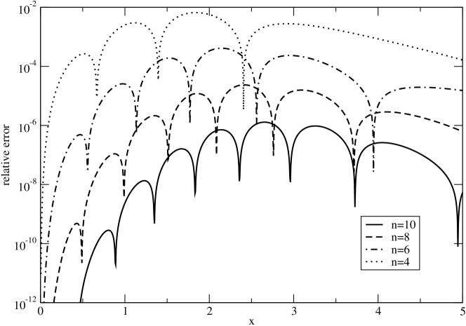
Figure 1: The relative error for a T-fraction approximation of the function $f_{\infty}(x)=\frac{\sqrt{\pi}}{2}{\rm e}^{-x^{2}}\left(i\,+\,{\rm erfi}(x)\right)$ as a function of the variable $x$ for the $n$th approximant.

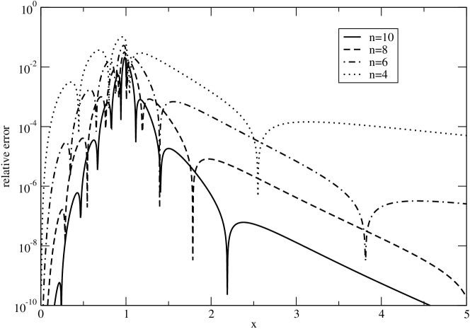
Figure 2: The relative error for a T-fraction approximation of the function $f_{0}(x)$, see Eq. (23), as a function of the variable $x$ for the $n$th approximant.

$\theta$	$H_{1}$	$H_{2}$	$H_{3}$	$H_{4}$	$H_{5}$
0.1	9.914(-1)	-1.0186	-0.3649	-0.2482	-0.2108
0.2	9.611(-1)	-1.0892	-0.4569	-0.2997	-0.1499
0.3	9.081(-1)	-1.1533	-0.4130	-0.0950	0.1268
0.5	7.790(-1)	-1.1037	-0.1000	0.1734	0.1217
0.8	6.116(-1)	-0.8336	0.1250	0.0939	-0.0075
1.0	5.289(-1)	-0.6692	0.1424	0.0403	-0.0133
1.5	3.888(-1)	-0.3970	0.0973	-0.0005	-0.0038
2.0	3.048(-1)	-0.2552	0.0581	-0.0038	-0.0007

Table 1: Expansion coefficients for the small $x$ expansion of the function $g(x)$, cf. Eq. (4).

$\theta$	$c_{-3}$	$c_{-5}$	$c_{-7}$	$c_{-9}$
0.1	1.387(-1)	6.368(-2)	3.897(-2)	2.810(-2)
0.2	1.537(-1)	8.275(-2)	6.256(-2)	5.856(-2)
0.3	1.749(-1)	1.130(-1)	1.071(-1)	1.305(0)
0.5	2.270(-1)	2.837(-1)	5.277(-1)	1.228(0)
0.8	3.153(-1)	4.418(-1)	8.723(-1)	2.509(0)
1.0	3.771(-1)	6.042(-1)	1.565(0)	5.580(0)
1.5	5.359(-1)	1.250(0)	4.777(0)	2.532(1)
2.0	6.979(-1)	2.143(0)	1.845(1)	7.639(1)

Table 2: Expansion coefficients for the large $x$ expansion of the function $g(x)$, cf. Eq. (5).

$\theta$	0	0.1	0.2	0.3	0.5	0.8	1.0	1.5	2.0
$b_{1}$	4.244(-1)	4.280(-1)	4.393(-1)	4.571(-1)	5.023(-1)	5.749(-1)	6.217(-1)	7.307(-1)	8.283(-1)
$a_{2}$	4.244(-1)	4.280(-1)	4.393(-1)	4.571(-1)	5.023(-1)	5.749(-1)	6.217(-1)	7.307(-1)	8.283(-1)
$b_{2}$	9.234(-1)	9.407(-1)	9.900(-1)	1.061(0)	1.224(0)	1.460(0)	1.608(0)	1.938(0)	2.223(0)
$a_{3}$	4.522(-1)	4.545(-1)	4.652(-1)	4.872(-1)	5.458(-1)	6.375(-1)	6.981(-1)	8.374(-1)	9.592(-1)
$b_{3}$	9.613(-1)	9.932(-1)	1.071(0)	1.184(0)	1.430(0)	1.731(0)	1.953(0)	2.413(0)	2.782(0)
$a_{4}$	4.702(-1)	4.730(-1)	4.792(-1)	5.074(-1)	5.879(-1)	6.695(-1)	7.673(-1)	9.678(-1)	1.117(0)
$b_{4}$	9.790(-1)	1.046(0)	1.135(0)	1.286(0)	1.650(0)	1.634(0)	2.168(0)	2.956(0)	3.388(0)
$a_{5}$	4.804(-1)	5.072(-1)	4.800(-1)	5.116(-1)	6.525(-1)	2.700(-1)	6.921(-1)	1.239(0)	1.409(0)
$b_{5}$	9.878(-1)	1.223(0)	1.177(0)	1.260(0)	2.046(0)	3.122(-1)	1.545(0)	3.720(0)	5.740(0)
$a_{6}$	4.865(-1)	7.067(-1)	4.471(-1)	3.718(-1)	9.483(-1)	-4.755(0)	7.390(-1)	2.021(0)	3.815(0)
$b_{6}$	9.923(-1)	3.713(0)	1.108(0)	5.128(-1)	5.835(0)	-4.275(0)	-8.132(-1)	8.054(-1)	-2.160(0)
$a_{7}$	4.902(-1)	3.404(0)	-2.049(-1)	-8.853(-1)	5.056(1)	8.397(-1)	4.991(0)	1.492(-2)	-2.648(0)
$b_{7}$	9.949(-1)	-4.507(-1)	4.077(-1)	-6.900(-1)	-8.928(-1)	9.416(-1)	5.566(0)	7.319(-3)	2.244(0)
$a_{8}$	4.926(-1)	4.519(-1)	2.686(0)	7.086(-1)	-8.812(-1)	-2.490(0)	-1.334(-3)	7.783(1)	1.698(0)
$b_{8}$	9.965(-1)	1.041(2)	-2.871(0)	7.651(-1)	7.850(0)	-2.190(0)	-1.653(-3)	7.817(1)	-1.833(0)

Table 3: Partial numerators $a_{i}$ and denominators $b_{i}$ for the T-fraction approximation of $g(x)$ as a function of the degeneracy parameter $\theta$, see Eq. (38). Note, that $b_{1}=a_{2}$.

Next, we turn to the general case of arbitrary degeneracy. Typical expansion coefficients $H_{i}$ are compiled in Tab. 1. Also, the expansion coefficients for large $x$ are given essentially by the Fermi integrals for order $l/2$. They are listed in Tab. 2 for various values of the degeneracy parameter $\theta$. Finally, the imaginary contribution due to the modified expression in Eq. (19) has to be determined. It reads

$$\mbox{Im}\,g(x) \approx \mbox{ln}\left(1+{\rm e}^{\eta}\right)\,-\,\frac{{\rm e}^{\eta}}{1+{\rm e}^{\eta}}\frac{x^{2}}{\theta}\,+\,\frac{{\rm e}^{\eta}}{2\left(1+{\rm e}^{\eta}\right)^{2}}\frac{x^{4}}{\theta^{2}}\,+\,\frac{{\rm e}^{\eta}\left({\rm e}^{\eta}-1\right)}{6\left(1+{\rm e}^{\eta}\right)^{3}}\frac{x^{6}}{\theta^{3}}$$ (29)

$$+\,\frac{{\rm e}^{\eta}\left(1-4{\rm e}^{\eta}+{\rm e}^{2\eta}\right)}{24\left(1+{\rm e}^{\eta}\right)^{4}}\frac{x^{8}}{\theta^{4}}\,+\,\frac{{\rm e}^{\eta}\left(-1+11{\rm e}^{\eta}-11{\rm e}^{2\eta}+{\rm e}^{3\eta}\right)}{120\left(1+{\rm e}^{\eta}\right)^{5}}\frac{x^{10}}{\theta^{5}}\,+\dots\,\,\,.$$

Using these coefficients, the T-fraction approximation is determined using the modified Q-D algorithm described in App. C. The resulting partial numerators and denominators are recorded in Tab. 3. The general form of the T-fraction considered here is

$$g(x) = \mbox{Re}\left[\begin{array}[]{c}\lx@intercol\hfil\mu_{0}\hfil\lx@intercol\vrule\lx@intercol\\ \hline\cr\vrule\lx@intercol\hfil x-ib_{1}\hfil\lx@intercol\end{array}\,+\,\begin{array}[]{c}\lx@intercol\hfil ia_{2}x\hfil\lx@intercol\vrule\lx@intercol\\ \hline\cr\vrule\lx@intercol\hfil x-ib_{2}\hfil\lx@intercol\end{array}\,+\,\begin{array}[]{c}\lx@intercol\hfil ia_{3}x\hfil\lx@intercol\vrule\lx@intercol\\ \hline\cr\vrule\lx@intercol\hfil x-ib_{3}\hfil\lx@intercol\end{array}\,+\,\begin{array}[]{c}\lx@intercol\hfil ia_{4}x\hfil\lx@intercol\vrule\lx@intercol\\ \hline\cr\vrule\lx@intercol\hfil x-ib_{4}\hfil\lx@intercol\end{array}\,+\,\dots\right]\,\,\,.$$ (38)

with $i$ being the imaginary unit, $\mu_{0}=2/3$.

IV Conclusions

It has been shown that T-fractions are a powerful method to obtain reliable and compact approximative expressions for the dielectric response of ideal plasmas at arbitrary degeneracy. In particular, a set of eight partial numerators and denominators are sufficient to obtain a satisfying accuracy for most practical applications. Fast implementations for the dynamic collision frequency and the self-energy in $GW$ approximations are possible based on these results due to a notable acceleration compared to a direct evaluation of the integral representation. An extension to bosonic systems appears to be straightforward and is work in progress.

Appendix A Small $x$ expansion coefficients

In order to regularize the hyper-singular integrals in Eq. (4), we consider an expansion of the Fermi function around zero

$$\frac{1}{\mbox{exp}(y^{2}/\theta-\eta)+1} = \frac{1}{1+{\rm e}^{-\eta}}\,-\,\frac{{\rm e}^{\eta}}{\left(1+{\rm e}^{\eta}\right)^{2}}\frac{y^{2}}{\theta}\,-\,\frac{{\rm e}^{\eta}\,\left({\rm e}^{\eta}-1\right)}{2\left(1+{\rm e}^{\eta}\right)^{3}}\frac{y^{4}}{\theta^{2}}\,-\,\frac{{\rm e}^{\eta}\,\left(1-4{\rm e}^{\eta}+{\rm e}^{2\eta}\right)}{6\left(1+{\rm e}^{\eta}\right)^{4}}\frac{y^{6}}{\theta^{3}}$$ (39)

$$-\,\frac{{\rm e}^{\eta}\left(-1+11\eta-11{\rm e}^{2\eta}+{\rm e}^{3\eta}\right)\,}{24\left(1+{\rm e}^{\eta}\right)^{5}}\frac{y^{8}}{\theta^{4}}\,+\,\dots\,\,\,.$$

The calculation has been done using the computer algebra software MATHEMATICA Mathematica6 . In detail, we obtain for the integrands

$$h_{2}(y) = \frac{1}{1+{\rm e}^{\eta}}\,\frac{1-{\rm e}^{y^{2}/\theta}}{1+{\rm e}^{y^{2}/\theta-\eta}}\,\,\,,$$ (40)

$$h_{3}(y) = \frac{1}{1+{\rm e}^{\eta}}\,\frac{\left(1+{\rm e}^{-\eta}\right)\,\left(1-{\rm e}^{y^{2}/\theta}\right)\,+\,\left(1+{\rm e}^{y^{2}/\theta-\eta}\right)y^{2}/\theta}{\left(1+{\rm e}^{-\eta}\right)\,\left(1+{\rm e}^{y^{2}/\theta-\eta}\right)}\,\,\,,$$ (41)

$$h_{4}(y) = \frac{{\rm e}^{\eta}}{2\left(1+{\rm e}^{\eta}\right)^{3}\left({\rm e}^{\eta}+{\rm e}^{y^{2}/\theta}\right)}\left[2\,-\,2{\rm e}^{2\eta+y^{2}/\theta}\,+\,{\rm e}^{\eta}\left(4+2y^{2}/\theta-y^{4}/\theta^{2}\right)\right.$$ (42)

$$\left.-{\rm e}^{y^{2}/\theta}\left(2-2y^{2}/\theta+y^{4}/\theta^{2}\right)\,+\,{\rm e}^{\eta+y^{2}/\theta}\left(-4+2y^{2}/\theta+y^{4}/\theta^{2}\right)\,+\,{\rm e}^{2\eta}\left(2+y^{2}/\theta+y^{4}/\theta^{2}\right)\right]\,\,\,,$$

$$h_{5}(y) = \frac{{\rm e}^{\eta}}{6\left(1+{\rm e}^{\eta}\right)^{4}\left({\rm e}^{\eta}\,+\,{\rm e}^{y^{2}/\theta}\right)}\,\left[-6\left(1+{\rm e}^{\eta}\right)^{3}\left(-1+{\rm e}^{y^{2}/\theta}\right)\right.$$ (43)

$$\left.+6\left(1+{\rm e}^{\eta}\right)^{2}\left({\rm e}^{\eta}+{\rm e}^{y^{2}/\theta}\right)y^{2}/\theta\,+\,3\left(-1+{\rm e}^{2\eta}\right)\left({\rm e}^{\eta}+{\rm e}^{y^{2}/\theta}\right)y^{4}/\theta^{2}\,+\,\left(1-4{\rm e}^{\eta}+{\rm e}^{2\eta}\right)y^{6}/\theta^{3}\right]\,\,\,,$$

with $H_{i}=\int_{0}^{\infty}\!dy\,h_{i}(y)/y^{2i-2}$. Also, for evaluating the integrals involved, it is convenient to determine the expansion of each integrand for small $x$ by reading off the corresponding terms in Eq. (39). Note, that the limits of $H_{i}$ in the non-degenerate and highly degenerate case are analytically known from the corresponding expansions of Eq. (7) and Eq. (8), respectively. Note also, that the values of $H_{1}$ and $H_{2}$ are given by Arista and Brandt Arista84 , while all higher expressions are given here for the first time.

Appendix B Large $x$ expansion coefficients

The Fermi integrals of order $l/2$ involved in the large $x$ expansion have been determined by MATHEMATICA Mathematica6 exploiting the relation of the Fermi integral to the polylogarithmic function Abramowitz72

$$F_{\alpha}(x) = -\Gamma(1+\alpha)\,\mbox{Li}_{1+\alpha}\left(-{\rm e}^{x}\right)\,\,\,.$$ (44)

The Fermi integrals $F_{-1/2},F_{1/2},F_{3/2},F_{5/2}$ can be easily obtained with the interpolation formulas given by Antia Antia93 .

Appendix C Modified Q-D algorithm

We summarize the modified Q-D algorithm introduced by de Andrade et al. Andrade03 . We start with the series expansions Eq. (17) and Eq. (18) and allow for zero coefficients $\mu_{i}$. Next, an auxiliary expansion is introduced by subtracting the expansion of the function $K/(1+z)$ with a free parameter $K$ from the above given expansion generating a new set of coefficients $\gamma_{i}$. For a convenient choice of $K$, all $\gamma_{i}$ will be non-zero and the ordinary Q-D algorithm can be applied. The continued fraction representation

$$\begin{array}[]{c}\lx@intercol\hfil\mu_{0}\hfil\lx@intercol\vrule\lx@intercol\\ \hline\cr\vrule\lx@intercol\hfil z-\beta_{1}^{(0)}\hfil\lx@intercol\end{array}\,-\,\begin{array}[]{c}\lx@intercol\hfil\alpha_{2}^{(0)}z\hfil\lx@intercol\vrule\lx@intercol\\ \hline\cr\vrule\lx@intercol\hfil z-\beta_{1}^{(0)}\hfil\lx@intercol\end{array}\,-\,\begin{array}[]{c}\lx@intercol\hfil\alpha_{3}^{(0)}z\hfil\lx@intercol\vrule\lx@intercol\\ \hline\cr\vrule\lx@intercol\hfil z-\beta_{3}^{(0)}\hfil\lx@intercol\end{array}\,-\,\begin{array}[]{c}\lx@intercol\hfil\alpha_{4}^{(0)}z\hfil\lx@intercol\vrule\lx@intercol\\ \hline\cr\vrule\lx@intercol\hfil z-\beta_{4}^{(0)}\hfil\lx@intercol\end{array}\,-\,\dots\,\,\,,$$ (53)

having the original series expansions Eq. (17) and Eq. (18) can be reconstructed from the coefficients $\gamma_{i}$ by the following algorithm:

• Determine $\gamma_{i}$ from a given set of $\mu_{i}$ and a convenient choice of $K$ as

  $$\gamma_{i} = \mu_{i}\,+\,\left(-1\right)^{i+1}K\,\neq\,0\,\,\,.$$ (54)

• Perform the Q - D algorithm

  $$\lambda_{i}^{(r)}\,=\,\delta_{i-1}^{(r+1)}\,+\,\lambda_{i-1}^{(r+1)}-\delta_{i-1}^{(r)} \delta_{i}^{(r)}\,=\,\lambda_{i}^{(r)}\delta_{i-1}^{(r-1)}/\lambda_{i}^{(r-1)}\,\,\,,$$ , (55)

  with the initialization

  $$\lambda_{1}^{(r)}\,=\,0 \delta_{1}^{(r)}\,=\,\frac{\gamma_{r}}{\gamma_{r-1}}\,\,\,,$$ , (56)

  and $i=2,3,\dots$, $r=\dots,-2,-1,0,1,2,\dots$.

• Determine for $i=1,2,\dots$ the following quantities leading to $\alpha_{i}$ and $\beta_{i}$,

  $$b_{i,i-1} = b_{i-1,i-2}\,-\,\left(\alpha_{i}+\beta_{i}\right)\,\,\,,$$

  $$d_{i,i-1} = d_{i-1,i-2}\,-\,\left(\lambda_{i}^{(0)}+\delta_{i}^{(0)}\right)\,\,\,,$$

  $$u_{i+1} = u_{i}\lambda_{i+1}^{(0)}\,\,\,,$$

  $$d_{i+1,0} = -d_{i,0}\delta_{i+1}^{(0)}\,\,\,,$$

  $$w_{i+1} = u_{i+1}\,+\,w_{i}\left(b_{i,i-1}-d_{i-1,i-2}-1\right)\,-\,u_{i}\left(d_{i,i-1}-b_{i-1,i-2}-1\right)\,\,\,,$$

  $$b_{i+1,0} = d_{i,0}\left[1-\frac{u_{i+1}}{w_{i+1}}\left(1\,-\,\frac{b_{i,0}}{d_{i+1,0}}\right)\right]^{-1}\,\,\,,$$

  $$\alpha_{i+1} = \frac{w_{i+1}}{w_{i}}\,\,\,,$$

  $$\beta_{i+1} = -\frac{b_{i+1,0}}{b_{i,0}}\,\,\,,$$

  with the initialization

  $$\alpha_{1}\,=\,0 \beta_{1}\,=\,\frac{\delta_{1}^{(0)}}{\gamma_{0}-K\delta_{1}^{(0)}}\,\,\,,$$ ,

  $$w_{1}\,=\,\mu_{0} u_{1}\,=\,\gamma_{0}\,\,\,,$$ ,

  $$b_{0,-1}\,=\,0 d_{0,-1}\,=\,0\,\,\,.$$ , (57)

Appendix D Numerics of continued fractions

There are several algorithms to numerically calculate the value of a continued fraction. Here, we use the backward recurrence algorithm which is known for its numerical stability Lorentzen92 . Given $n$ partial numerators $a_{i}$ and partial denominators $b_{i}$, we determine an approximation $t_{0}$ to the continued fraction by setting $t_{n}$ to a small, non-zero number and perform the iteration

$$t_{i-1} = \frac{a_{i}}{b_{i}+t_{i}}\,\,\,,$$ (58)

for $i=n,\dots,1$.

References

- (1) J. Lindhard, Mat.-Fys. Medd.-K. Dan. Vidensk. Selsk. 28, (8) (1954).
- (2) G.D. Mahan, Many-Particle Physics (Plenum Press, New York, 1993).
- (3) S. Ichimaru, Statistical Plasma Physics (Addison-Wesley, Reading, 1994).
- (4) N.R. Arista and W. Brandt, Phys. Rev. A 29, 1471 (1984).
- (5) H.R. Griem, Principles of Plasma Spectroscopy (Cambridge University Press, Cambridge, 1997).
- (6) H. Reinholz, R. Redmer, G. Röpke, and A. Wierling, Phys. Rev. E 62, 5648 (2000).
- (7) see e.g. H. Mori, Prog. Theor. Phys. 34, 399 (1965); M.H. Lee, Phys. Rev. Lett. 49, 1072 (1982); J. Horáček and T. Sasakawa, Phys. Rev. C 32, 70 (1985); D.E. Neuenschwander, Am. J. Phys. 62, 871 (1994).
- (8) G.A. Baker, Padé Approximants (Cambridge Univ. Press, Cambridge, 1996).
- (9) G.A. Baker and J.L. Gammel, The Padé approximant in theoretical physics (Academic Press, New York, 1970).
- (10) W.J. Thron, Bull. Amer. Math. Soc. 54, 206 (1948).
- (11) J.H. McCabe and J.A. Murphy, J. Inst. Maths Applics 17, 233 (1976).
- (12) B.D. Fried and S.D. Conte, The Plasma Dispersion Function (Academic, New York, 1961).
- (13) M. Abramowitz and I.A. Stegun, Handbook of Mathematical Functions (Dover, New York, 1972).
- (14) P. Henrici, Applied and Computational Complex Analysis, Vol. 2 (Wiley, New York, 1991)
- (15) E.X.L. de Andrade, J.H. McCabe, and A. Sri Ranga, J. Comp. Appl. Math. 156, 487 (2003).
- (16) J.H. McCabe, Math. Comp. 28, 811 (1974).
- (17) J.H. McCabe, J. Plasma Physics 32, 479 (1984).
- (18) Wolfram Research, Inc., Mathematica, Version 6.0, Champaign, IL (2007).
- (19) H.M. Antia, Ap. J Suppl. 84, 101 (1993).
- (20) L. Lorentzen and H. Waadeland, Continued Fractions with Applications (North-Holland, Amsterdam, 1992).