Complex Langevin dynamics at finite chemical potential:
mean field analysis in the relativistic Bose gas
Gert Aarts
Department of Physics, Swansea University, Swansea, United Kingdom
Email
g.aarts@swan.ac.uk
Abstract:
Stochastic quantization can potentially be used to simulate theories with
a complex action due to a nonzero chemical potential. We study complex
Langevin dynamics in the relativistic Bose gas analytically, using a mean
field approximation. We concentrate on the region with a Silver Blaze
problem and discuss convergence, stability, fixed points, and the
severeness of the sign problem. The real distribution satisfying the
extended Fokker-Planck equation is constructed and its nonlocal form is
explained. Finally, we compare the mean field results in finite volume
with the numerical data presented in Ref. [1].
Lattice Quantum Field Theory, Lattice QCD
††preprint: arXiv:0902.4686 [hep-lat]
1 Introduction
Theories with a complex action are not easy to solve numerically, since
approaches based on importance sampling break down. This is commonly
referred to as the sign problem. An important theory in this class is QCD
at finite baryon chemical potential, with a complex fermion determinant
satisfying .111In case of a complex
chemical potential, this relation becomes .
Several methods have been devised to circumvent the sign problem in QCD,
mostly at small chemical potential and in the vicinity of the crossover
between the confined and the deconfined phase
[2, 3, 4, 5, 6, 7, 8, 9, 10, 11, 12, 13, 14]. For a
detailed lattice QCD study of the sign problem at small chemical
potential, see Ref. [15]. Considerable insight in the QCD
sign problem has also been obtained with Random Matrix Theory
[16, 17, 18, 19, 20, 21].
In some theories the sign problem can be eliminated altogether, using a
reformulation in terms of different degrees of freedom
[22, 23, 24].
Since stochastic quantization [25] does not rely on
importance sampling, it can potentially be applied to theories with a
complex action using complex Langevin dynamics
[26, 27]. Studies in the 80’s, however, have
given mixed results, see e.g. Refs. [28, 29].
For an extensive review and more references, see Ref. [30]. Recently the approach was reconsidered as a method
to solve nonequilibrium quantum fields dynamics in Minkowski spacetime
[31, 32, 33]. It was shown that
instabilities, which plagued earlier studies, can be controlled by using
small enough Langevin stepsizes. Moreover, insight in the convergence
properties of the method can be obtained from features of classical flow
diagrams. Other recent applications include PT symmetric theories
[34] and unbounded actions [35]. In
Ref. [36] we applied stochastic quantization to various
theories with a nonzero chemical potential. In particular, we considered
QCD with static quarks, in which the fermion determinant is approximated
but the full gauge dynamics is preserved. First results on a lattice
are encouraging. The required extension from SU(3) to SL(3,)
is discussed in detail.
The sign problem in QCD at finite chemical potential does not arise
because of the anticommuting nature of the quark fields. Also
in bosonic theories with a nonzero chemical potential and an
action that behaves under complex conjugation as , the
sign problem appears. In
Ref. [1] we considered the relativistic Bose gas (a self
interacting complex scalar field) in four dimensions in the presence of a
chemical potential as one of the simplest examples of a relativistic
field theory with a severe sign problem. Like QCD, this theory has a
Silver Blaze problem [37]: at strictly zero temperature and
small chemical potential, bulk physical observables are independent of the
chemical potential, even though it enters explicitly in the microscopic
dynamics. At larger chemical potential, the system enters a Bose condensed
phase. The independence below onset and the formation of a state
with nonzero density above onset is similar to what is expected to occur
in QCD at zero temperature. It was demonstrated in Ref. [1] that complex Langevin dynamics reproduces the expected
physics, on lattices of size , with . The sign problem
was shown to be severe. However, no obstacles related to the sign problem,
the Silver Blaze problem, or in taking the thermodynamic limit were
encountered.
In this paper we complement the numerical study of Ref. [1] with a detailed analytical study in the mean field
approximation. We concentrate on the region with the Silver Blaze problem.
The paper is organized as follows. In Sec. 2 we remind the
reader of the model and the corresponding complex Langevin equations. In
order to prepare for the mean field analysis, we first discuss the case
without interactions. In Sec. 3 we summarize the exact
results in the free field limit, using standard field theory. Subsequently
the free Langevin equations are solved analytically, both for continuous
and discretized dynamics. We discuss convergence and stability properties.
In Sec. 4 the stationary solution of the Fokker-Planck
equation is given, again ignoring interactions, and shown to be in
agreement with the solution of the Langevin equations in the limit of
large Langevin time.222Recently, an interesting approach to study
stationary solutions of complex Langevin dynamics was presented in Ref. [38]. The criterium for convergence is derived from
this distribution as well. We find that the real probability distribution
is highly nonlocal and explain why. In Sec. 5 interactions
are included and the analysis is extended to the mean field approximation.
We derive fixed points of the mean field Langevin equations at finite
Langevin stepsize. Finally the mean field predictions in finite volume are
compared with the nonperturbative results obtained by complex Langevin
simulations [1]. The appendix contains a short remark
about lattice dispersion relations.
2 Relativistic Bose gas and Langevin dynamics
We consider a self-interacting complex scalar field in the presence of a
chemical potential , with the continuum action
(2.1)
The euclidean action is complex and satisfies . We take , so that at
vanishing and small the theory is in its symmetric phase.
We study this theory on the lattice, with the action
(2.2)
As always, chemical potential is introduced as an imaginary constant
vector
potential in the temporal direction [39].
The number of euclidean dimensions is , the lattice spacing , and the lattice four-volume is , where
() are the number of sites in a spatial (temporal)
direction. We use periodic boundary conditions.
In order to formulate the complex Langevin equations for this theory, the
complex field is first written in terms of two real fields
() as . The lattice action
then reads
(2.3)
We use the antisymmetric tensor , with
, ,
and summation over repeated indices is implied throughout.
Since the Boltzmann weight in the partition function,
(2.4)
is complex, the theory has a sign problem and one
cannot rely on importance sampling. Writing the weight as , one may consider the phase quenched theory
(2.5)
where is the real part of the action in Eq. (2.3), i.e. the
term proportional to is dropped. By analysing the average phase
factor in the phase quenched theory, , it
was shown in Ref. [1]
that this theory has a severe sign problem: at nonzero chemical
potential the average phase factor goes to zero exponentially fast in the
thermodynamic limit.
We use stochastic quantization. The Langevin
equations for the fields read
(2.6)
where is the Langevin time. The noise is Gaussian and normalized as
(2.7)
Since the force in Eq. (2.6) is complex, the fields are complexified as
(2.8)
The complex Langevin equations we consider in this paper then read
(2.9)
(2.10)
The noise is chosen to be real.
The drift terms are defined as
(2.11)
(2.12)
and read explicitly
(2.13)
(2.14)
Observables are written in terms of the complexified fields (2.8) as well. We consider the square of the field modulus,
(2.15)
and the density , given
by , with
After complexification all observables have a real and
imaginary part.
Employing that the noise is random, we observe that the Langevin
equations have the following symmetry,
(2.17)
for all and similar with 1 and 2 interchanged.
Under this transformation, the drift terms change as
(2.18)
Correlation functions odd under this transformation should
vanish after noise averaging, which implies that
(2.19)
The nonzero combinations are
(2.20)
Applying this to the expectation values of the observables in Eqs. (2.15, LABEL:eq:dens), we find that they are purely real. This is
indeed what was observed numerically in Ref. [1].
3 Ignoring interactions
In order to set the stage for the mean field analysis, we first solve
the Langevin dynamics without interactions (),
allowing for a detailed understanding of convergence and
stability properties in the Silver Blaze regime.
3.1 Standard results
We start by summarizing the results obtained in the standard field theory
approach (see e.g. Ref. [40]). After going to momentum space,
according to
(3.1)
where , with , and , with , the action (2.3)
reads
(3.2)
where
(3.3)
and333In the formal continuum limit
, .
(3.4)
Note that , , and that is nonhermitian.
The phase quenched theory is obtained by taking .
Up to an irrelevant constant, the logarithm of the partition function is
(3.5)
The observables we are interested in are given by
(3.6)
and
(3.7)
where , .
As always, the severeness of the sign problem is estimated by the average
phase factor in the phase quenched theory, given
by the ratio of the partition functions of the full and phase quenched
theories (2.4, 2.5),
(3.8)
where , the difference between the corresponding free
energy densities, is given by
(3.9)
Note that this can be easily generalized to arbitrary powers of the phase
factor in theories with nonvanishing phase factors.444
Define the partition function
.
Then
,
with
Finally, since the eigenvalues of in the action (3.2) are
, the theory
without interactions exists provided that . This yields the
standard stability criterium for a free Bose gas at finite chemical
potential,
(3.10)
corresponding to in the formal continuum limit.
We restrict the analysis below therefore to the case that ;
this is the Silver Blaze region.
3.2 Continuous Langevin dynamics
We now solve the complex Langevin equations to compare the outcome with
the results given above. The Langevin equations (2.9, 2.10) read in momentum space
(3.11)
(3.12)
where the noise is normalized as
(3.13)
Ignoring interactions, we find for the drift terms
(3.14)
(3.15)
where and are defined in Eq. (3.4) above.
In terms of
(3.16)
the Langevin dynamics is written as
(3.17)
The matrix can be diagonalized by an orthogonal
transformation and has doubly degenerate eigenvalues . The solution of the Langevin equations is
(3.18)
(3.19)
where denote the initial conditions.
We are now in a position to discuss the convergence properties of the
Langevin process in the limit of large Langevin time. First we note that
there is independence of initial conditions provided that , i.e. in the region of interest here. Taking , we
find for the two-point functions, after using Eq. (3.13) and
performing the Langevin time integrals,
(3.20)
Most of the terms vanish in the limit that
, again provided that . The surviving terms are
(3.21)
The structure of these two-point functions is in agreement with
the symmetry (2.17, 2.20) discussed above.
For the observables we find the following.
The square of the field modulus (2.15) is given by
(3.22)
which agrees with Eq. (3.6).
After going to momentum space, the density (LABEL:eq:dens) reads
(3.23)
which agrees with Eq. (3.7). Note that all two-point
functions in Eq. (3.21) contribute to this answer.
We conclude therefore that the Langevin process is independent of initial
conditions and converges to the correct result in the limit of infinite
Langevin time, provided that , as required in the Silver Blaze
region. Moreover, the complexification is essential, as exemplified by the observables above.
3.3 Discretized Langevin dynamics
We proceed by briefly considering the Langevin process after discretizing
Langevin time as , where is the Langevin time step.
The discretized Langevin equations are
(3.24)
(3.25)
and the noise obeys .
In the notation of Eq. (3.16), these equations are summarized
as
(3.26)
and solved by
(3.27)
where is the initial condition.
Convergence is determined by the eigenvalues of . This yields the
condition
(3.28)
resulting in the constraint
(3.29)
We find that the convergence criterium is modified by an explicit
stepsize dependence. However, this restriction is not special for the
complex Langevin process [41, 30].
Consider real Langevin dynamics at zero or in the
phase quenched theory. In both cases and the criterium reads
(3.30)
Since is maximal at the edge of the Brillouin zone (), this yields the modest constraint (for )
(3.31)
At nonzero chemical potential, this constraint is modified to
(3.32)
both in the full and the phase quenched theory.
In the Silver Blaze region, where is bounded,
this leads to only a slightly stronger bound on .
However, since this bound is determined by ultraviolet modes at the scale of the lattice cutoff, it is likely that
a similar constraint holds in the high-density phase as well. In the limit that , exponentially small stepsizes would eventually be required. It should be noted, however, that
for such large chemical potentials lattice artefacts are severe.
The solution (3.27) can be used to study finite stepsize
effects in two-point functions at infinite Langevin time.
We come back to this below using a more elegant approach
based on fixed points of the Langevin equations.
4 Fokker-Planck equation
In order to better understand the Langevin process, we now study
properties of the associated distributions.
Consider first the Langevin process (2.6) and the distribution
, defined via
(4.1)
where the brackets on the LHS denote noise averaging.
The distribution satisfies the Fokker-Planck equation (in continuous Langevin time)
(4.2)
As always, the index is summed over.
The stationary solution,
(4.3)
always exists. However, since the action is complex, this is not the probability
distribution for the complex Langevin process.
More relevant for the complexified process (2.9, 2.10) we
consider here, is the real distribution
, defined via [26]
(4.4)
This distribution satisfies the extended Fokker-Planck equation
(4.5)
If stochastic quantization is applicable for complex actions, the two
expectation values (4.1) and (4.4) should be equal [26].
We focus on the stationary solution of Eq. (4.5) and henceforth
drop the dependence. Ignoring again interactions, the stationary
solution should satisfy
(4.6)
where the drift terms were given in Eqs. (3.14, 3.15).
Explicitly, this reads
(4.7)
Based on the structure of the equation, the solution can be written as
(4.8)
where is a normalization constant.
Inserting this expression in Eq. (4.7) yields the
coefficients
(4.9)
We have therefore found the stationary distribution corresponding to the
complex Langevin process in the noninteracting case.555See Refs. [42, 43] for other examples.
Note that since , the distribution is real in
real space, as it should be.
We now verify that this stationary solution is indeed the
distribution corresponding to the Langevin process in the limit of
infinite Langevin time.
Performing the Gaussian integrals, we find the partition
function
(4.10)
where is an irrelevant constant and
(4.11)
The two-point functions that follow from this distribution are
(4.12)
These agree exactly with the results obtained by solving the Langevin
equation, cf. Eq. (3.21).
The theory with the probability distribution
exists provided that the eigenvalues of the quadratic form in Eq. (4.8) are positive. We find the eigenvalues to be
(4.13)
These are positive provided that . The criterium that determines
the convergence of the Langevin dynamics also emerges in the stationary
solution of the extended Fokker-Planck equation, as expected.
Let us discuss some more properties of the distribution (4.8).
First we note that the distribution is highly nonlocal in real space and
does not allow for e.g. a derivative expansion, due
to the division by in the coefficients
(4.9). We find therefore that the complexity of the original
local weight has been traded for the nonlocality of the real
probability distribution. However, this nonlocal behaviour is expected: it
follows from the Langevin equations that the modes with are purely
real, i.e. . This is enforced in the
probability distribution by the singular behaviour as . For the
same reason the limit is singular, since there is no need to
complexify the dynamics in this case and the distribution for the
modes should reduce to a delta function, .
These considerations fix the dependence on .
In conclusion, we have found the stationary solution of the extended
Fokker-Planck distribution. The real distribution is nonlocal and
singular in the limit that .
5 Mean field approximation
We now return to the interacting theory, with discretized Langevin time , and
consider the two-point functions
(5.1)
Using the Langevin equations (3.24, 3.25), we find
that these correlation functions evolve according to
(5.2)
Here we used that ,
since the fields at time do not depend on the noise at time . The
terms proportional to are finite stepsize corrections.
We then look for fixed points of the Langevin equations, and put
(5.3)
etc. This yields the fixed point equations
(5.4)
To implement a mean field approximation and find a self-consistent set for the two-point functions
(5.1), we factorize the interaction terms. Consider for example the term appearing in the drift term (2.14). We write
(5.5)
Using the notation
(5.6)
the drift terms in the mean field approximation read
(5.7)
(5.8)
These can be further simplified by noting that both and are proportional to , for all Langevin times.
We write therefore
(5.9)
such that the drift terms reduce to
(5.10)
(5.11)
with
(5.12)
Since and depend explicitly on the Langevin time, the time-dependent mean field Langevin equations cannot be solved analytically.666In fact, the problem is now very similar to that of nonequilibrium field dynamics using a self-consistent mean field approximation in the equal-time formalism [44].
We therefore look for fixed points. After substituting Eqs. (5.10, 5.11) in the fixed point equations (5.4) and performing some algebra, we find that at the fixed point and that the two-point functions can be decomposed as
(5.13)
This is in agreement with the symmetry (2.17, 2.20). The three fixed point equations (5.4) then become
(5.14)
The solution is
(5.15)
For vanishing Langevin stepsize this simplifies to
(5.16)
while in the phase quenched theory () where real Langevin dynamics
is applicable, the solution reduces to
(5.17)
We find finite stepsize corrections linear in , as expected
[41]. Furthermore, we note that for large stepsize the
denominator in the first line of Eq. (5.15) can go negative.
However, this occurs precisely when the stability criterium (3.29)
is violated (after the replacement ) and is therefore
excluded.
The expressions in Eq. (5.16) agree precisely with the solutions
(3.21) obtained by solving the Langevin equations without
interactions, after making the mean field replacement .
This replacement corresponds to the standard mean field approximation in
which the mass parameter receives a tadpole correction,
(5.18)
or, in the notation of this section,
(5.19)
with
(5.20)
These equations define a self-consistent gap equation for . Given
and , the gap equation can be solved numerically after
specifying the lattice size. For example, taking , we find
and at on a lattice of size
. The critical chemical potential then follows from (or
) and is found to be
.777When , follows from (or
), yielding for .
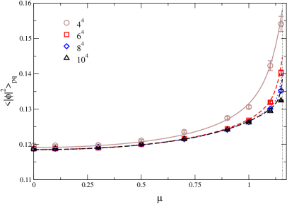
Figure 1:
The lines represent the mean field results for in the
full (left) and phase quenched (right) theories for various lattice sizes,
taking . The vertical dotted line indicates the mean field
estimate for the critical chemical potential. The data points are obtained
with Langevin simulations [1].
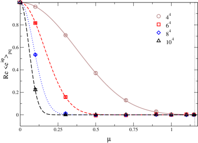
Figure 3:
Left: as in Fig. 1 for the average phase factor in the
phase quenched theory . Right: difference
between the free energy densities of the full and the phase
quenched theories in the mean field approximation.
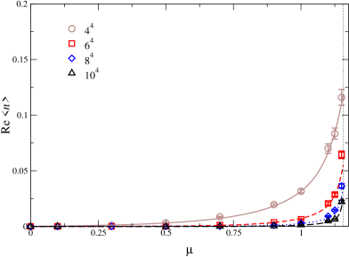
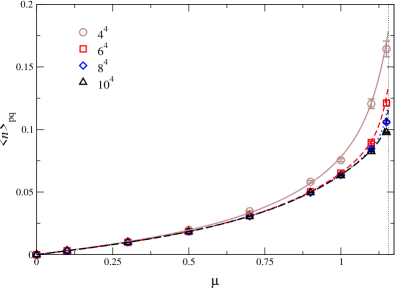
We have solved the gap equation in the Silver Blaze region and used the
outcome to compute and in the mean field
approximation as a function of chemical potential for different lattice
sizes. The results are shown in Figs. 1 and 2
respectively, for . The vertical dotted lines indicate the
mean field estimate of the critical chemical potential. In the full theory
(figures on the left) the expected independence emerges in the
thermodynamic limit. In the phase quenched theory (figures on the right),
observables depend on , since there is no Silver Blaze feature, see
Appendix A. Also shown in these plots are data points
obtained from the numerical solution of the Langevin process, with
stepsize [1]. We observe
surprisingly good agreement between the mean field and the nonperturbative
results for all values of the chemical potential and all lattice sizes
considered, indicating that the mean field approximation captures the most
relevant interactions.
In Fig. 3 we show the average phase factor in the phase
quenched theory (left) and the difference
between the free energy densities, given in Eq. (3.9), again after the replacement . As already
mentioned, the sign problem is severe in the thermodynamic limit: taking
e.g. and a lattice volume , we find that the
average phase factor
is indeed exponentially small.
To conclude this section, we note that it is straightforward to adapt the
stationary solution of the extended Fokker-Planck equation, constructed in
Sec. 4, to the mean field approximation discussed here.
Since in the mean field approximation only two-point functions appear, the
mean field probability distribution remains of the form (4.8)
with the simple replacement (or ). Existence of
the Fokker-Planck distribution in the Silver Blaze region now requires
.
6 Conclusion
In order to further understand the applicability of complex Langevin
dynamics for theories with a complex action due to finite chemical
potential, we have studied the relativistic Bose gas in the Silver Blaze
region analytically. Ignoring interactions, we have investigated
convergence and stability, and constructed the stationary solution of the
extended Fokker-Planck equation. We explained why this real probability
distribution is nonlocal in real space. Subsequently, interactions were
included on the mean field level and the fixed point of the mean field
Langevin equations with finite stepsize was derived. We gave a comparison
between the mean field predictions and the nonperturbative numerical data
from Ref. [1] in the Silver Blaze region. Surprisingly
good agreement was found for all values of the chemical potential
considered, including finite size effects, indicating that the mean field
approximation captures the most important effects of the interactions. We
have demonstrated analytically that the sign problem is severe for lattice
volumes used in this study. From the combination of results obtained here
and in Ref. [1], it can be argued that complex Langevin
dynamics in the Silver Blaze region is well understood in this theory.
One obvious next step is to extend the analysis to the high-density phase,
which requires the introduction of the mean field
(note that ).
Finally, it would be interesting to apply mean field approximations to
other theories as well, especially in combination with numerical studies.
In particular, this would be useful for QCD with static quarks
[36].
Acknowledgments.
I thank Kim Splittorff, Ion-Olimpiu Stamatescu and Simon Hands for their
interest and discussion. This work is supported by an STFC Advanced
Fellowship.
Appendix A Dispersion relation
The propagator corresponding to the action (3.2) is
(A.1)
Dispersion relations follow from the poles of the propagator,
taking . We find
(A.2)
where
(A.3)
This can be written as
(A.4)
such that the (positive energy) solutions are
(A.5)
just as in the continuum theory. Lattice discretization effects only
appear in the dispersion relation at zero chemical potential, .
The critical value is , so
that one mode becomes exactly massless at the transition.
The phase quenched theory corresponds to . In
the formal continuum limit, the phase quenched theory is a theory with a
real action and mass parameter . The dispersion relation is
(A.6)
corresponding to in the continuum limit,
as anticipated.
These results are easily extended to the self-consistent mean field approximation, where the mass parameter receives a tadpole correction and is replaced by .
References
[1]
G. Aarts,
Phys. Rev. Lett. 102 (2009) 131601
[0810.2089 [hep-lat]].
[2]
Z. Fodor and S. D. Katz,
Phys. Lett. B 534 (2002) 87
[hep-lat/0104001].
[3]
Z. Fodor and S. D. Katz,
JHEP 0203 (2002) 014
[hep-lat/0106002].
[4]
Z. Fodor, S. D. Katz and K. K. Szabo,
Phys. Lett. B 568 (2003) 73
[hep-lat/0208078].
[5]
Z. Fodor and S. D. Katz,
JHEP 0404 (2004) 050
[hep-lat/0402006].
[6]
C. R. Allton et al.,
Phys. Rev. D 66 (2002) 074507
[hep-lat/0204010].
[7]
C. R. Allton, S. Ejiri, S. J. Hands, O. Kaczmarek, F. Karsch,
E. Laermann and C. Schmidt,
Phys. Rev. D 68 (2003) 014507
[hep-lat/0305007].
[8]
C. R. Allton et al.,
Phys. Rev. D 71 (2005) 054508
[hep-lat/0501030].
[9]
R. V. Gavai and S. Gupta,
Phys. Rev. D 68 (2003) 034506
[hep-lat/0303013].
[10]
P. de Forcrand and O. Philipsen,
Nucl. Phys. B 642 (2002) 290
[hep-lat/0205016].
[11]
P. de Forcrand and O. Philipsen,
Nucl. Phys. B 673 (2003) 170
[hep-lat/0307020].
[12]
P. de Forcrand and O. Philipsen,
JHEP 0701 (2007) 077
[hep-lat/0607017].
[13]
M. D’Elia and M. P. Lombardo,
Phys. Rev. D 67 (2003) 014505
[hep-lat/0209146].
[14]
Z. Fodor, S. D. Katz and C. Schmidt,
JHEP 0703 (2007) 121
[hep-lat/0701022].
[15]
S. Ejiri,
Phys. Rev. D 78 (2008) 074507
[0804.3227 [hep-lat]].
[16]
J. C. Osborn,
Phys. Rev. Lett. 93 (2004) 222001
[hep-th/0403131].
[17]
G. Akemann, J. C. Osborn, K. Splittorff and J. J. M. Verbaarschot,
Nucl. Phys. B 712 (2005) 287
[hep-th/0411030].
[18]
J. C. Osborn, K. Splittorff and J. J. M. Verbaarschot,
Phys. Rev. Lett. 94 (2005) 202001
[hep-th/0501210].
[19]
K. Splittorff and J. J. M. Verbaarschot,
Phys. Rev. Lett. 98 (2007) 031601
[hep-lat/0609076].
[20]
J. Han and M. A. Stephanov,
Phys. Rev. D 78 (2008) 054507
[0805.1939 [hep-lat]].
[21]
J. C. R. Bloch and T. Wettig,
JHEP 0903 (2009) 100
[0812.0324 [hep-lat]].
[22]
S. Chandrasekharan and U. J. Wiese,
Phys. Rev. Lett. 83 (1999) 3116
[cond-mat/9902128].
[23]
M. G. Endres,
Phys. Rev. D 75 (2007) 065012
[hep-lat/0610029].
[24]
S. Chandrasekharan,
PoS LATTICE2008 (2008) 003
[0810.2419 [hep-lat]].
[25]
G. Parisi and Y. s. Wu,
Sci. Sin. 24 (1981) 483.
[26]
G. Parisi,
Phys. Lett. B 131 (1983) 393.
[27]
J. R. Klauder and W. P. Petersen,
SIAM J. Numer. Anal. 22 (1985) 1153;
J. Stat. Phys. 39 (1985) 53.
[28]
F. Karsch and H. W. Wyld,
Phys. Rev. Lett. 55 (1985) 2242.
[29]
J. Ambjorn, M. Flensburg and C. Peterson,
Nucl. Phys. B 275 (1986) 375.
[30]
P. H. Damgaard and H. Hüffel,
Phys. Rept. 152 (1987) 227.
[31]
J. Berges and I. O. Stamatescu,
Phys. Rev. Lett. 95 (2005) 202003
[hep-lat/0508030].
[32]
J. Berges, S. Borsanyi, D. Sexty and I. O. Stamatescu,
Phys. Rev. D 75 (2007) 045007
[hep-lat/0609058].
[33]
J. Berges and D. Sexty,
Nucl. Phys. B 799 (2008) 306
[0708.0779 [hep-lat]].
[34]
C. W. Bernard and V. M. Savage,
Phys. Rev. D 64 (2001) 085010
[hep-lat/0106009].
[35]
C. Pehlevan and G. Guralnik,
Nucl. Phys. B 811, 519 (2009)
[0710.3756 [hep-th]].
[36]
G. Aarts and I. O. Stamatescu,
JHEP 0809 (2008) 018
[0807.1597 [hep-lat]].
[37]
T. D. Cohen,
Phys. Rev. Lett. 91 (2003) 222001
[hep-ph/0307089].
[38]
G. Guralnik and C. Pehlevan,
arXiv:0902.1503 [hep-lat].
[39]
P. Hasenfratz and F. Karsch,
Phys. Lett. B 125 (1983) 308.
[40]
J.I. Kapusta, Finite-temperature field theory, Cambridge University
Press (1994).
[41]
G. G. Batrouni, G. R. Katz, A. S. Kronfeld, G. P. Lepage, B. Svetitsky and K. G. Wilson,
Phys. Rev. D 32 (1985) 2736.
[42]
J. Ambjorn and S. K. Yang,
Phys. Lett. B 165 (1985) 140.
[43]
H. Nakazato and Y. Yamanaka,
Phys. Rev. D 34 (1986) 492.
[44]
G. Aarts, G. F. Bonini and C. Wetterich,
Phys. Rev. D 63 (2001) 025012
[hep-ph/0007357].