How well do starlab and nbody4 compare? I: Simple models

Abstract

N-body simulations are widely used to simulate the dynamical evolution of a variety of systems, among them star clusters. Much of our understanding of their evolution rests on the results of such direct N-body simulations. They provide insight in the structural evolution of star clusters, as well as into the occurrence of stellar exotica. Although the major pure N-body codes STARLAB/KIRA and NBODY4 are widely used for a range of applications, there is no thorough comparison study yet.

Here we thoroughly compare basic quantities as derived from simulations performed either with STARLAB/KIRA or NBODY4.

We construct a large number of star cluster models for various stellar mass function settings (but without stellar/binary evolution, primordial binaries, external tidal fields etc), evolve them in parallel with STARLAB/KIRA and NBODY4, analyse them in a consistent way and compare the averaged results quantitatively. For this quantitative comparison we develop a bootstrap algorithm for functional dependencies.

We find an overall excellent agreement between the codes, both for the clusters’ structural and energy parameters as well as for the properties of the dynamically created binaries. However, we identify small differences, like in the energy conservation before core collapse and the energies of escaping stars, which deserve further studies.

Our results reassure the comparability and the possibility to combine results from these two major N-body codes, at least for the purely dynamical models (i.e. without stellar/binary evolution) we performed. Further detailed comparison studies for more complex systems, e.g. including stellar/binary evolution, are required.

1 Introduction

In recent years, stellar dynamics has led to an advance in a variety of fields, such as studies of individual star clusters (Hurley et al. 2005), star cluster systems (Vesperini et al. 2003), populations of “exotic” objects in star clusters (e.g. runaway merger products with masses of up to few thousands solar masses, Portegies Zwart et al. 2004; blue stragglers, Hurley et al. 2005; Portegies Zwart et al. 2007), the formation and evolution of higher-order hierarchical systems (triples, quadruples and higher, e.g. van den Berk et al. 2007), the Galactic centre and runaway stars (Gualandris et al. 2005; Baumgardt et al. 2006; Löckmann & Baumgardt 2008), etc.

The major codes used in this field are the family of nbodyx codes (Aarseth 1999; the most widely used versions are nbody4, nbody6, nbody6++, the most recent version being nbody7) and the starlab environment with its N-body integrator kira (Portegies Zwart et al. 2001). Despite these codes being widely used, there is no thorough comparison study yet. First attempts have been initiated by Douglas Heggie and others at the IAU General Assembly 1997 in Kyoto (therefore, the “Kyoto experiment”), however until today, the number of results and their analysis is small (see Heggie 2001 and http://www.maths.ed.ac.uk/$\sim$heggie/kyotoII/kyotoII.html for descriptions of this collaborative experiment and some of its results).

Although the fundamental integration scheme (4^th order, block-timestep “Hermite” predictor-corrector scheme, see Makino & Aarseth 1992, the next section in this paper, or Aarseth 2003 for a variety of technical details) is the same for both codes, severe differences in the treatment of binaries, stellar and binary evolution are present, plus naturally different implementations of otherwise comparable components.

With this paper we start a series of publications to study the impact of differences in the input physics onto the results from both codes. We start with the most simple models, not including stellar evolution, external tidal fields or primordial binaries. More complex models, without the aforementioned restrictions, will be studied in upcoming papers of this series.

In these studies we concentrate on the statistical treatment of a large number of runs, represented by its median values and uncertainty ranges, as the results of single runs will naturally diverge due to the amplification of numerical errors (Goodman et al. 1993). This holds for two models with slightly different initial configurations and evolved with the same code, as well as the same initial model evolved with two different codes. We will not compare wall-clock times for the different runs (as this is dependent on a multitude of parameters, software and hardware settings), or parameters usually only relevant to code developers. Instead we want to provide the interested scientific user a guideline to the comparability of the codes studied and point at differences concerning parameters likely relevant for the user.

The paper is organised as follows: Sect. 2 gives an overview of similarities and differences of the starlab and nbody4 input physics. Sect. 3 describes the general model setup and the data analysis pipeline. In Sect. 4 we introduce a bootstrap approach to quantify differences between functions. In Sect. 5 we present our results for a range of mass function settings. Energy conservation is studied in Sect. 6, core collapse in Sect. 7, and the properties of stars becoming unbound during cluster evolution in Sect. 8. We finish this paper with our conclusions in Sect. 9.

2 Overview

2.1 Similarities in input physics: N-body integrator scheme

Almost all recent direct N-body integrators (including nbody4 and kira/starlab) are based on the 4^th order, block-timestep “Hermite” predictor-corrector scheme (but see e.g. Nitadori & Makino 2008 for higher-order N-body integrators).

“Hermite” predictor-corrector scheme: This integration scheme was first described by Makino (1991). It is based on individual timesteps for every star, (approximate) prediction of all stars’ positions and derivatives, and (accurate) calculation and correction (using Hermite interpolation) for a subset of stars at any given timestep.

More specifically, the scheme comprises of the following steps to evolve one star $i$ from the present time $t_{0}$ to the time $t_{1}=t_{0}+\Delta t$. The positions, velocities, acceleration and the first time derivative of the acceleration at time $t_{0}$ are assumed to be known for all stars. This description follows Makino & Aarseth (1992).

1. Predict/extrapolate the positions, velocities, accelerations and the first time derivatives of the acceleration at time $t_{1}$, using Taylor expansion (up to 4^th order for the positions) with the quantities at time $t_{0}$, for all stars.

2. Calculate for star $i$ the acceleration and the first time derivative of the acceleration at time $t_{1}$, based on the predicted positions and velocities of all stars.

3. Calculate for star $i$ the second and third time derivatives of the acceleration at time $t_{0}$, using the acceleration and the first time derivative of the acceleration at times $t_{0}$ and $t_{1}$.

4. Calculate for star $i$ the correction to the predicted position and velocity, based on the second and third time derivatives of the acceleration at time $t_{0}$.

Block timesteps: In principle, the optimum timestep can be estimated for each star individually, based on this star’s acceleration and its time derivatives. In reality, it is computationally favourable to group stars with approximately the same timestep together, and evolve whole “blocks” of stars at once. This treatment reduces the overheads otherwise needed to calculate the predicted positions and velocities of all stars. Conventionally, block timesteps of power-of-2 ($\Delta t_{n}\propto 1/2^{n}$) are used.

2.2 Differences in input physics: Treatment of binaries

The treatment of binaries is one of the challenges in N-body simulations. While especially close binaries are dynamically important (e.g. star-binary and binary-binary interactions can eject stars from the cluster core, resulting in the halting of core collapse and leading to core re-expansion), their relevant timescale is the orbital period (of the order of days), while the relevant timescale for the cluster as a whole is the crossing timescale (of the order of Myrs). A “brute force” approach would need to set the timestep to a fraction of the orbital period to evolve the binary accurately, which would immediately stall the calculation (and corrupt energy conservation due to exponential growth of numerical inaccuracies).

However, especially close/hard binaries are hardly perturbed by external effects, as their binding energy is high compared to the energy injected by external perturbations. Such binaries evolve essentially as in isolation.

nbody4 uses the KS (Kustaanheimo & Stiefel 1965) and CHAIN (Mikkola & Aarseth 1993) regularisation techniques to follow close encounters between stars. The basic idea of these regularisation methods is to switch to special coordinate systems together with appropriate time transformations which significantly improve the overall energy conservation during close encounters.

starlab separates between “unperturbed/hard binaries” and “perturbed binaries”, where the distinction is made where the dimensionless perturbation (i.e. the ratio of the external perturbation to the internal binary binding energy) reaches a critical value (typically 10^-6). Unperturbed binaries are evolved solving analytically the Kepler equations, and their components are treated as point masses, for the purpose of influencing other stars.

“Slightly perturbed” bound pairs with a dimensionless perturbation between 10^-6 and 10^-5 are treated with a “slowdown” algorithm similar to the one described in Mikkola & Aarseth (1996).

More strongly perturbed pairs and multiples are treated as resolved into their components for the purpose of determining their influence of surrounding stars. Their motion is calculated directly.

Perturbations are followed efficiently by keeping a perturber-list for each binary.

More detailed information are given in Portegies Zwart et al. (2001)

3 Model setup and data analysis

In order to simplify future comparisons with other N-body codes, we provide the input snapshots (both in starlab/kira as well as in nbody format),the time evolutions of important cluster parameters, and for each code an example run parameter file on our webpage (http://www.phys.uu.nl/$\sim$anders/data/ NBODY_STARLAB_Comparison/ and http://members.galev.org/nbody/ NBODY_STARLAB_Comparison/).

We created 50 input models per setting, using the appropriate starlab tasks, to improve the statistics. For nbody4, these models were converted into the appropriate input format, to have maximum comparability.

All input models were evolved for 1000 N-body time units, well beyond core collapse, using nbody4 (the May 2008 version from Aarseth’s webpage) respectively starlab/kira (throughout the paper we use starlab version 4.4.2). All simulations were performed on PCs hosting GRAPE special-purpose hardware (see e.g. Makino et al. 2003; the nbody4 runs were performed on a machine hosting a GRAPE6A board, the starlab on a machine hosting a GRAPE6BLX board). As nbody6 does not support the usage of GRAPE hardware, we limit our analysis to nbody4 in the course of this paper. For the impact of the hardware (and the associated internal calculation accuracy) on the results of our N-body simulations, see Anders (2008). Preliminary results indicate little impact.

Crucial for our comparison is a self-consistent analysis of the nbody4 and starlab/kira output. In order to achieve this goal we convert the starlab output into the nbody4 output format (with the same number of significant digits = 15), removing all information not available for the nbody4 output, like local densities, binary parameters, energies, cluster centres etc. At this stage the binary tree structure is not yet established and the binary/multiple components are treated as single stars.

The results, snapshot by snapshot, were then fed into starlab/kira and evolved for a short time (a 1/32^th of an N-body time unit), in order to reconstruct the binary populations. From the resulting snapshots we calculate a large number of diagnostics: structural parameters (cluster centres, mass profile, Lagrange radii, King parameter, core density etc), energies (potential energy, kinetic energy, energy error etc), and parameters of dynamically created binaries (eccentricities, binding energies, positions of the binaries inside the cluster etc).

For the majority of this paper we will concentrate on the results from snapshots with fully reconstructed binary tree structure. The impact of the binary tree reconstruction on the data will be discussed in Sect. 5.4.

3.1 Nomenclature

We will use the following definitions and abbreviations throughout the paper.

• standard runs = std: simulations made with the standard settings described in Sect. 3.2

• MF10 runs: simulations made with the standard settings described below, except that a Salpeter (1955) mass function is used, with the upper mass limit being 10x larger than the lower mass limit

• MF100 runs: simulations made with the standard settings described below, except that a Salpeter (1955) mass function is used, with the upper mass limit being 100x larger than the lower mass limit

• unperturbed binaries: relative external perturbation is smaller than 10^-6

• perturbed binaries: relative external perturbation is larger than 10^-6, but binding energy $\arrowvert{\rm E}_{\rm bind}\arrowvert\geq 0.5$ kT.

• multiples: second strongest bound orbit in a multiple system (primary mass = total mass of inner binary with strongest bound orbit)

• significance level of statistical test results:

  • highly significant: p-value $<$ 1%

  • significant: p-value $<$ 5%

  • weakly significant: p-value $<$ 10%

In the remainder of this work, for studying structural parameters and energies we will use only the median cluster parameters calculated from the individual runs. The associated uncertainty ranges are the 16%/84% quantiles (similar to the 1$\sigma$ ranges for Gaussian-distributed quantities around their mean value), divided by the square-root of the number of runs contributing, to estimate the uncertainty in the position of the median value. For studying the properties of dynamically created binaries, we add up all binaries from the individual runs which are present at a given time.

This procedure reduces the noise from the individual runs. In addition, as runs inevitably diverge (either two start models with slightly different initial conditions evolved with the same code, or one start model evolved with two different codes), a direct comparison of individual runs is not expected to give meaningful results.

3.2 Benchmark tests: The “standard runs”

The benchmark test settings (further on referred to as “standard runs”) we propose are the following:

1. 1024 (=1k) particles

2. equal mass system

3. no primordial binaries

4. no stellar/binary star evolution

5. Plummer (1911) sphere density profile

6. no external tidal field

These settings constitute the most simple configuration, which is likely available for testing in every future N-body code.

In further sections/papers, several of the restrictions imposed to establish the benchmark test settings are going to be dropped, in order to get more realistic cluster models.

4 Difference of functions & Bootstrap test

In our study we will obtain time evolutions of various parameters, as computed for a variety of settings. We want to compare these time evolutions quantitatively and determine the statistical significance of differences. For the former one we define a measure how different two functional relations are, for the latter one we introduce a version of bootstrapping, adapted to such functional dependencies.

4.1 Difference of functions: The distance measure

Assume we have two functional dependencies of one parameter from the independent variable $x$: $y_{1}(x)$ and $y_{2}(x)$. For each $x$ these dependencies have uncertainties $\sigma_{1}(x)$ and $\sigma_{2}(x)$. For example, from our studies, this relates to $y_{1}(x)=r_{core}^{NBODY}(time)$ and $y_{2}(x)=r_{core}^{STARLAB}(time)$ (i.e. the core radius at a given time, as determined from nbody respectively starlab simulations) and the related uncertainties.

If the data have asymmetric error bars $\sigma_{1}^{+}(x)$ and $\sigma_{1}^{-}(x)$, e.g. originating from the use of quantiles, we suggest to use an average $\sigma_{1}(x)=0.5\cdot(\sigma_{1}^{+}(x)+\sigma_{1}^{-}(x))$. However, other measures are possible and, as long as consistency is ensured, should give similar results.

The relative difference between the functional dependencies at a given $x$ is then:

$$\delta_{12}(x)=\frac{y_{1}(x)-y_{2}(x)}{\sqrt{\sigma_{1}(x)^{2}+\sigma_{2}(x)^{2}}}$$ (1)

We then define the “difference between functions 1 and 2” as

$$\Delta_{12}=\frac{1}{N}\cdot\left|\sum_{x}\delta_{12}(x)\right|$$ (2)

where $N$ is the number of datapoints used for the statistic. We consider only the absolute value, as we want to have a measure of the size of the difference, but not necessarily its direction. In addition, this ensures $\Delta_{12}\equiv\Delta_{21}$.

Equivalently we define the “absolute difference between functions 1 and 2” as

$$\Gamma_{12}=\frac{1}{N}\cdot\sum_{x}\left|\delta_{12}(x)\right|$$ (3)

While $\Delta_{12}$ is more sensitive to systematic offsets, $\Gamma_{12}$ traces also statistical fluctuations.

4.2 Bootstrap test for comparing functions

We calculate 3 $\times$ 300 test clusters with starlab using the same analysis routines as for the other clusters. These clusters follow the same settings as the main simulations (i.e. 300 clusters for each respective mass function).

From these test clusters we randomly select sets of 50 clusters each (i.e. the number of clusters in the main simulations) with replacement, and calculate for each parameter the median $y^{T}(x)$ and quantiles $\sigma^{T}(x)$.

We build 2000 such sets. Out of those we randomly select two sets (again with replacement) and derive the individual values of $\Delta_{12}^{T}$ and $\Gamma_{12}^{T}$. We repeat this procedure 10000 times to estimate the $\Delta_{12}^{T}$ and $\Gamma_{12}^{T}$ test distributions for each parameter. As all test clusters are calculated with the same settings, the $\Delta_{12}^{T}$ and $\Gamma_{12}^{T}$ test distributions represent the null hypothesis “functions 1 and 2 are drawn from the same parent distribution”. By comparing these test distributions with the values derived from the main simulations $\Delta_{12}^{S}$ and $\Gamma_{12}^{S}$ we can quantify the fraction of data in the test distribution with $\Delta_{12}^{T}$ or $\Gamma_{12}^{T}$ more deviating than the values derived from the main simulations $\Delta_{12}^{S}$ or $\Gamma_{12}^{S}$. This value serves as measure of how similar the two main simulations are.

In order to evaluate if the 300 test clusters were sufficient, we performed the same analysis with a subset of 250 test clusters for the “MF10” setting. Depending on the parameter studied, the resulting comparability p-values differ on average by $\pm$1% up to maximum deviations of $\pm$3%. None of these differences changed the significance level of any of the results, though.

In order to avoid applying the test statistic to highly correlated data, which appears for the earliest timesteps (as the nbody4 and starlab/kira runs share the same start models) and which is beyond the area of application of the test statistic, we start the summation in Eq. 2 and 3 at 10 N-body time units. This value is a compromise between avoiding early correlated data and containing the core collapse phase for all models. We tested our method with a range of starting times and find in general very good agreement. On average differences are $\sim$3%, for few extreme cases up to $\sim$15%, with a trend of increasing offsets with increasing starting times. This changes only occasionally the classification of the test result into the significancy level categories defined in Sect. 3.1, mainly in cases where the p-value already is close to a boundary between such categories.

5 Results

5.1 Results for the “standard runs”

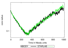
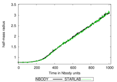
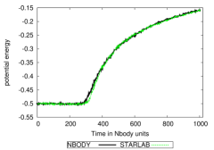
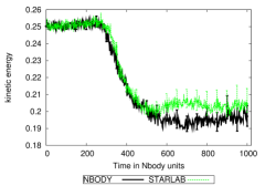
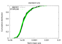
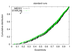
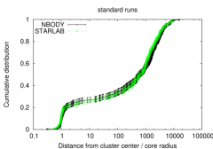
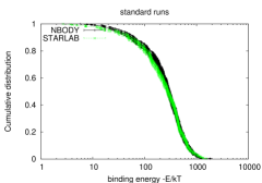
Figure 1: Comparison of “standard runs” simulations using starlab (green/grey) vs nbody4 (black). The lines show the median values, the error bars give the uncertainty ranges from the 50 individual runs. Shown are the time evolutions of the core radius (top left), half-mass radius (top right), potential energy (bottom left) and kinetic energy (bottom right).

Figure 2: Comparison of binary parameters from “standard runs” after 1000 N-body time units (=well after core collapse) using starlab (green/grey) vs nbody4 (black). Shown are the cumulative distributions of the semi-major axis (top left), the eccentricity (top right), the distance from the cluster centre (in units of the cluster’s core radius; bottom left) and the binding energy (bottom right). The lines show the data, the error bars give the uncertainty ranges from bootstrapping. For the eccentricity, the prediction for a thermal distribution (e²) is overplotted.

Fig. 2 (top left) shows that core-collapse occurs at around 320 N-body time units. This coincides well with the often-used criterion of the first occurrence of a binary with binding energy higher than 100 kT (see Table 3). At the same time, other structural parameters start to change as well (e.g. the cluster’s half-mass radius, shown in Fig. 2, top right), as the occurrence of hard binaries starts heating the cluster core, propagating outwards, resulting in an irreversible overall expansion of these rather low-mass clusters.

At the time of core collapse, also both kinetic and potential energy of the cluster as a whole change their behaviour: the potential energy increases, while the kinetic energy decreases slightly, as energy gets increasingly locked up in binaries (Fig. 2, lower panels). This effect will be studied further in Sect. 5.4, where the effects of rebuilding the binary tree structure is discussed.

The results obtained with starlab and with nbody4 lie for most studied parameter within the combined uncertainty ranges. However, for some parameters small systematic offsets seem to be present. To test their significance we developed a bootstrapping algorithm for comparing functions, described in Sect. 4.

The results from this bootstrapping test are presented in Table 1. In this Table we give for various parameters the fraction of test runs made with the same settings (i.e. representing the null hypothesis of a unique parent distribution) that are more deviating (i.e. which have larger $\Delta_{12}$ respectively $\Gamma_{12}$) than the results for this parameter from the main simulations using nbody4 or starlab.

Except for the total energy E_tot (and the conservation of the total energy $\delta$E_tot), which will be discussed below (Sect. 6), solely the core radius evolutions (and quantities calculated from the core radius) are significantly discrepant. This discrepancy originates from a kink in the median temporal core radius evolution for the nbody4 simulations. This kink could not be traced back to any kink/jump in individual runs (on the contrary, some starlab runs have stronger jumps than any of the nbody4 runs). We rather expect this kink to be an unfortunate cumulative stochastic effect. This is supported by the fact that after the kink the temporal dependencies from starlab and nbody4 continue to evolve in parallel, though offset by the amount the kink caused. The differences in the evolutions of the kinetic energies appear to be larger than for the core radii, however, as also the uncertainties are larger these differences are not statistically significant.

In Fig. 2 we study the distribution of the parameters describing the dynamically created binaries. For the 1k standard runs core collapse occurs at approximately 320 N-body time units (see Fig. 2 and Table 3). We show the parameter distributions of binaries present at 1000 N-body time units, hence well after core collapse. The shown error bars are estimated from 10000 bootstrap realisations of each dataset. Visually, the distributions compare well.

In order to quantify differences between the parameter distributions using either starlab or nbody4 we used a Kuiper test (Kuiper 1962, i.e. an advanced KS test, for KS test see e.g. Numerical Recipes Press et al. 1992). The results are presented in Table 2. Given are the total numbers of binaries per set of simulations and the Kuiper test results in %. A Kuiper test result is the probability that 2 distributions are drawn from the same parent distribution. Some of the results seem to be inconsistent with being drawn from the same parent distribution. However, we have performed a large number of comparisons with the Kuiper test. This unavoidably leads to the problem of multiple testing, which can basically be understood such that if we perform 100 independent tests, a fraction of the order of $10\%$ of p-values below $0.1$ will arise by chance even if none of the null hypothesis of the tests would be wrong. Moreover, the small p-values occur for tests with sample sizes $\approx 50$, which is just at the lower limit for reliable results with the Kuiper test. Hence, in view of the small number of ”significantly small” p-values (these are marked coloured in Table 2), we conclude that we do not find significant evidence for deviations of interesting size of the properties of dynamically created binaries from nbody4 and starlab simulations.

We also tested the eccentricity distributions against the common assumption of a thermal distribution, which is an eccentricity distribution $\sim$ 2*e, or a cumulative distribution $\sim$ e². A thermal distribution is generally expected based on phase space arguments (see e.g. Heggie 1975). The results are given in the last two columns of Table 2 for starlab and nbody4 respectively, and show good agreement with a thermal distribution. However, cumulative distributions of higher polynomial order than e² are not rejected either by the Kuiper test. We therefore used the binary data obtained as by-product from the calculations of the bootstrap test clusters, using starlab only. The number of runs is a factor 6 higher than for our main simulations, hence statistics also for the binaries is greatly enhanced (total number of binaries is 2018, compared to 323 for the main simulations). We test their cumulative eccentricity distributions against a number of power-law distributions e^α. For the STD test clusters we find a range in $\alpha$ = 2.1 – 2.8 with Kuiper test probabilities $>$ 10%, with a probability $>$ 95% for $\alpha$ = 2.3 – 2.5, hence significantly biased towards larger eccentricities than a thermal distribution would predict (a thermal distribution has a Kuiper test probability = 4.16%, hence is significantly rejected).

We split the whole sample in thirds, based on the semi-major axis, the distance from the cluster centre and the binding energy. However, due to the reduction of the number of binaries in each of these subsets, the Kuiper test does not reject the null hypothesis of the eccentricity distributions being thermal on a significant level (except for the subset of binaries with intermediate semi-major axes, which has a p-value of 2.5%). The p-value curves are too broad to derive any trends.

The general agreement between the data obtained using either starlab or nbody4 is good.

The distributions just after core collapse give comparable results (except for the spatial distribution, as the binaries did not yet have enough time to escape the cluster centre significantly), although the number of binaries is smaller (i.e. statistics is poorer).

5.2 Results for the “MF10 runs”

The results for the “MF10 runs” are presented in Fig. 4 - 4.

For these simulations core collapse occurs at around 60-70 N-body time units (see Fig. 4 [upper left panel] and Table 3). Qualitatively both the structural behaviour and the properties of the binaries compare well with the standard case, except for the speed up the mass function causes. Only the binary binding energies are higher as compared to the standard runs (by a factor $\sim$ 2), although the form of the cumulative distribution of the binding energies is comparable.

Both the bootstrap test for structural/energy parameters (except for the energy conservation, see Sect. 6) and the Kuiper test for the binary properties prove the very good agreement between the results obtained from the nbody4 and starlab simulations.

We tested again the hypothesis of a thermal eccentricity distribution of the dynamically created binaries. For both the nbody4 and the starlab main runs, the Kuiper test yields probabilities which do not reject the hypothesis of a thermal eccentricity distribution. Again, we used the binary data obtained as by-product from the calculations of the bootstrap test clusters, using starlab only. The total number of binaries is 1207, compared to 191 for the main simulations. We test their cumulative eccentricity distributions against a number of power-law distributions e^α. For the MF10 test clusters we find a range in $\alpha$ = 2.4 – 3.0 with Kuiper test probabilities $>$ 10%, with a maximum probability = 80.7% for $\alpha$ = 2.8, hence significantly biased towards larger eccentricities than a thermal distribution would predict (a thermal distribution has a Kuiper test probability = 0.06%, hence is highly significantly rejected).

We again split the whole sample in thirds, now also based on the primary mass and the mass ratio. We find that binaries with small semi-major axis, high binding energy or massive primaries tend to favour distributions closer to a thermal distribution than binaries with large semi-major axis, low binding energy or low-mass primaries. This can qualitatively be understood by assuming those binaries to be the ones with the most past encounters, hence the higher probability to thermalise. While the binaries with large semi-major axis, low binding energy or low-mass primaries are still highly significantly rejected, binaries with high binding energy are highly significantly rejected, binaries with high primary mass are weakly significantly rejected and binaries with small semi-major axis are not rejected to be consistent with a thermal distribution. The distance from the cluster centre (both binaries close to the cluster centre and in the far cluster outskirts are significantly rejected) and the mass ratio of the binary ($\sim$10 per cent, i.e. very weakly significantly rejected) have only small effects.

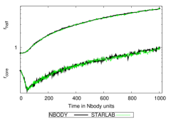
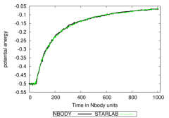
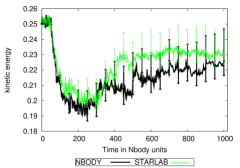
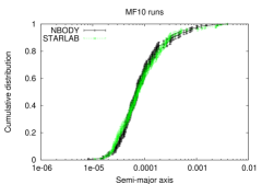
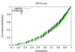
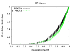
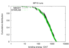
Figure 3: Comparison of “MF10 runs” simulations using starlab (green/grey) vs nbody4 (black). The lines show the median values, the error bars give the uncertainty ranges from the 50 individual runs. Shown are the time evolutions of the core radius (top left, bottom lines), half-mass radius (top left, top lines), the mean object mass in the core (top right), potential energy (lower left panel) and kinetic energy (bottom right).

Figure 4: Comparison of binary parameters from “MF10 runs” after 1000 N-body time units (=well after core collapse) using starlab (green/grey) vs nbody4 (black). Shown are the cumulative distributions of the semi-major axis (top left), the eccentricity (top right), the secondary-to-primary mass ratio (bottom left) and the binding energy (bottom right). The lines show the data, the error bars give the uncertainty ranges from bootstrapping.

5.3 Results for the “MF100 runs”

The results for the “MF100 runs” are presented in Fig. 6 - 6.

For these simulations core collapse occurs at around 20 N-body time units (see Fig. 6 [upper left panel] and Table 3), the wider mass function (compared to “MF10” runs) further speeding up the evolution. Qualitatively both the structural/energy parameters and the properties of the binaries compare well with the standard case. Only the binary binding energies are again higher as compared to the “MF10” runs, and the cumulative distribution of the binding energies is steeper, biased to higher energies. In general, the MF100 runs show larger scatter compared to the other runs. This is due to the larger stochastic effects for the highest masses caused by the wider mass range.

Both the binary properties and the structural/energy parameters are in good agreement. Weakly significant inconsistency is found for the half-mass radius and the potential energy evolution only. For these runs, even the energy conservation is not inconsistent, as the main differences occur only before core collapse, at ages which are largely removed by skipping the first 10 N-body time units for the bootstrapping.

For the MF100 test clusters we also test the eccentricity distribution of unperturbed binaries (again for the test statistics clusters, hence 485 clusters instead of 62 clusters in the main simulations) against various power-law relations and find a range in $\alpha$ = 1.9 – 3.0 with Kuiper test probabilities $>$ 10%, with a plateau of probability $>$ 95% for $\alpha$ = 2.3 – 2.6. A thermal distribution has a Kuiper test probability = 28.1%, hence can not be rejected.

We again split the complete sample in thirds and employ Kuiper tests to quantify the probability of the subsamples’ eccentricity distribution being thermal. Binaries are consistent with a thermal eccentricity distribution for: small semi-major axes, high binding energies, high primary mass, large distances from the cluster centre and (to a lesser extend) large mass ratios. For each of those subsets when compared with a thermal distribution a Kuiper test gives p-values $\ga$ 80 per cent. Except for the small mass ratio subset (which is comparable with a thermal distribution at p-value $\approx$ 40 per cent) for the opposite subsets a thermal distribution is at least weakly significantly, if not more strongly, rejected.

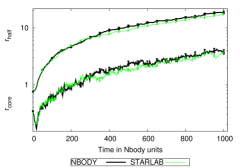
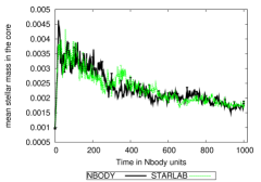
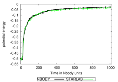
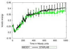
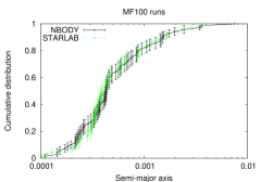
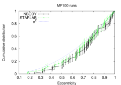
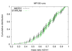
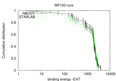
Figure 5: Comparison of “MF100 runs” simulations using starlab (green/grey) vs nbody4 (black). The lines show the median values, the error bars give the uncertainty ranges from the 50 individual runs. Shown are the time evolutions of the core radius (top left, bottom lines), half-mass radius (top left, top lines), the mean object mass in the core (top right), potential energy (lower left panel) and kinetic energy (bottom right).

Figure 6: Comparison of binary parameters from “MF100 runs” after 1000 N-body time units (=well after core collapse) using starlab (green/grey) vs nbody4 (black). Shown are the cumulative distributions of the semi-major axis (top left), the eccentricity (top right), the secondary-to-primary mass ratio (bottom left) and the binding energy (bottom right). The lines show the data, the error bars give the uncertainty ranges from bootstrapping.

5.4 Using starlab “MF10 runs” to test for possible biases introduced by analysis procedure

We checked whether the binary reconstruction with starlab/kira introduced spurious effects.

The structural parameters are largely unaffected. Minor differences in the binary parameters originate in the inclusion of perturbed binaries into the sample before full binary reconstruction.

The main differences occur for the energies. Before binary reconstruction, binaries are treated as 2 separate stars. Their orbital velocities contribute therefore to the total kinetic energy of the cluster. Their binding potential energy constitutes a significant part of the clusters total potential energy. In the case of a fully reconstructed binary tree structure both the orbital velocities’ kinetic energies and the binding potential energies are treated separately from the total cluster values, leading to an apparent “loss” of total energy.

However, the temporal parameter evolutions derived from starlab vs nbody4 simulations show very similar bootstrap results both before and after the binary reconstruction. We therefore conclude that the binary reconstruction does not lead to systematical changes.

In addition, we checked whether the splitting into and analysis of single snapshots introduces systematic differences. We pass the full 1000-snapshots starlab output through the starlab analysis routine hsys_stats (like we do for the single snapshots) and statistically compare the results with the results from the single-snapshot approach. We find slight differences induced by the resetting of the centre-of-mass for the single-snapshot approach, of which none is statistically significant (except for the centre-of-mass itself). Likewise, the binaries (both perturbed and unperturbed) do not show significant differences. Alone the multiples’ properties show significant differences (due to the spurious reconstruction of a small number of multiples far out of the cluster centre), and should be treated with caution.

6 Energy conservation

Ideally, the total energy should be constant during each simulation (except for the locking up of energy in binaries), and hence also in the median datasets. In practice, numerical inaccuracies lead to changes in the total energy. This energy error can be seen e.g. as the change of total energy per N-body time unit. These errors are larger if higher accuracy and hence more timesteps per N-body time unit are required, e.g. during core collapse and close encounters.

After core collapse, the energy error rises steeply, indicating that after core collapse, the errors are dominated by close encounters and binaries (and more timesteps per N-body unit are required). Prior to core collapse the errors originate from inaccuracies of the Hermite integrator alone. For ages well after core collapse, the energy error steadily decreases as the cluster expands and the number of timesteps per N-body unit drops.

The energy conservation from nbody4 shows roughly the same shape as the one from starlab (see Fig. 7). However, before core collapse the energy conservation from nbody4 is systematically worse than from starlab, roughly a factor 3 – 10, with median deviations of 4 – 5 ($\sim$2 – 3 for MF100). After core collapse, the median deviations are for all sets of simulations well below a factor 2. However, the overall scatter strongly increases (by factors 30 – 2000) due to the non-conservative numerical effects during binary interactions. Interestingly, the starlab data show similar energy conservation compared to the nbody4 data, despite the much more sophisticated and programming expensive regularisation treatment in nbody4.

Performing an integration with the KS routines switched off shows that the larger energy errors of nbody4 prior to core collapse come from the KS formalism (possibly from the interface between the main integrator and the KS algorithm), although no details or solutions could be found. However, the energy conservation in nbody4 is still good, and clearly sufficient for most applications.

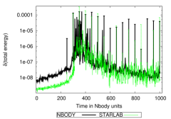
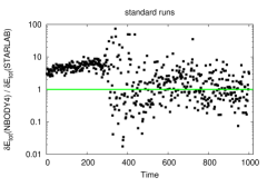
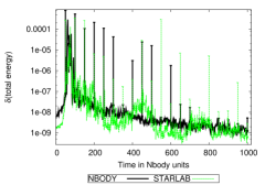
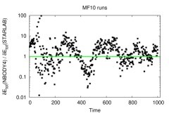
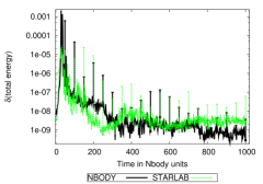
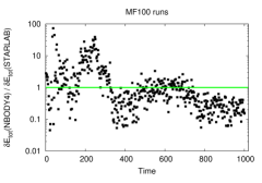
Figure 7: The energy conservation for nbody4 (black lines) and starlab (green lines) for: “standard runs” (top), “MF10 runs” (middle), and “MF100 runs” (bottom). The right panels show the respective energy error ratios nbody4/starlab. A horizontal lines as y=1 is added, to guide the eye.

Table 1: Results from the bootstrap test. Given are the fractions (in %) of the test distributions more deviating than the main simulations, i.e. the smaller this number the less alike the distributions are. For details see text.

parameter	std	MF10	MF100
	$\Delta_{12}$ $\Gamma_{12}$	$\Delta_{12}$ $\Gamma_{12}$	$\Delta_{12}$ $\Gamma_{12}$
rcore	10.79 7.84	59.56 83.17	24.99 27.37
rhalf	43.79 66.70	36.39 56.13	9.8 7.8
rmax	80.74 40.58	21.77 25.85	25.26 26.73
$<$mass${}_{\rm core}>$	28.70 77.44	79.56 76.81	92.18 83.38
$\arrowvert$ density centre $\arrowvert$	94.25 99.41	95.24 58.26	91.26 94.32
Epot	40.10 83.08	59.52 78.82	5.60 6.16
Ekin	32.43 39.08	48.54 56.38	68.97 77.52
Etot	0.86 0.72	45.64 47.75	80.35 98.17
$\delta$Etot	0 0	0 0	58.13 99.18

Table 2: Kuiper test results. Given is the probability (in %) that for the given setup the binary properties from starlab vs. nbody4 are drawn from the same distribution. Quantities are: axis = semi-major axis, ecc = eccentricity, D1 = distance of the binary from cluster centre, in units of the core radius, , D2 = distance of the binary from cluster centre, in units of the half-mass radius, E/kT = binding energy in E/kT, m2/m1 = mass ratio secondary mass / primary mass. #1 = number of binaries in the starlab simulation, #2 = number of binaries in the nbody4 simulation. In addition, e${}^{2}_{SL}$ and e${}^{2}_{NB}$ are the probabilities, that respectively the starlab/nbody4 data for the eccentricity distributions are compatible with a cumulative distribution of the form e² (equivalent to a thermal eccentricity distribution $\sim$ 2*e). For a description of the setups see text.

setup	#1	#2		axis	ecc	D1	D2	E/kT	m2/m1		e${}^{2}_{SL}$	e${}^{2}_{NB}$
STD, unperturbed	333	322		39.7	99.5	42.7	76.4	66.2	100.0		99.8	99.5
STD, perturbed	31	24		91.8	99.5	96.3	99.9	88.0	100.0		95.6	97.4
STD, multiples	10	9		9.6	99.4	85.0	99.8	20.7	100.0		99.9	99.9
MF10, unperturbed	191	192		41.6	92.5	81.4	87.2	84.8	14.9		29.3	82.2
MF10, perturbed	50	37		94.8	60.4	58.8	3.3	80.6	50.3		99.5	99.1
MF10, multiples	14	15		33.9	57.4	32.2	37.4	37.4	30.5		95.2	99.8
MF100, unperturbed	62	68		70.8	65.8	14.4	63.7	99.2	16.8		95.1	94.7
MF100, perturbed	36	44		17.3	98.5	77.7	95.8	24.7	9.8		99.1	86.0
MF100, multiples	29	33		81.1	52.2	39.9	83.7	68.5	91.6		99.9	99.0

7 Core collapse

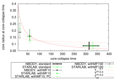
Figure 8: Comparison of simulations using starlab (green/grey) vs nbody4 (black). Shown is the time at which core collapse occurs (i.e. the time at which the first binary with more than 100 kT binding energy is formed) vs the “depth” of core collapse (i.e. the core radius at core collapse time).

For the three settings investigated in this study (i.e. “standard”, “MF10” and “MF100”), the parameters of core collapse are presented in Fig. 8 and Table 3. For each setting, the values as derived from starlab are consistent within the 1$\sigma$ uncertainties with the values as derived from nbody4.

We find a power-law dependence between time and “depth” of core collapse, with $\alpha\sim$ -0.3 $\pm$ 0.2. This behaviour can be understood qualitatively as follows: Core collapse is driven by the most massive stars, which are sinking towards the centre of the cluster on a timescale that is a fraction 1/M of the relaxation time. Hence core collapse will occur faster in clusters with a broader mass spectrum. For clusters with more massive stars, the core also reaches a state where finite-N effects become important. At the same time core collapse is halted at lower densities since energy generation due to binaries becomes more efficient for higher mass binaries.

Table 3: Values of core collapse, i.e. at the time when the first binary with binding energy $>$ 100 kT occurs. Given are the time of core collapse t_cc, and the core radius at this time r_c,cc. Shown are the median value from the individual runs, the uncertainty ranges are the 16 and 84 quantiles, equivalent to 1$\sigma$ ranges of the mean.

setup	tcc	rc,cc
STD, starlab	332${}_{-39}^{+25}$	0.086${}_{-0.025}^{+0.026}$
STD, nbody4	316${}_{-26}^{+42}$	0.087${}_{-0.026}^{+0.027}$
MF10, starlab	59${}_{-11}^{+9}$	0.155${}_{-0.042}^{+0.056}$
MF10, nbody4	60${}_{-8}^{+8}$	0.159${}_{-0.033}^{+0.050}$
MF100, starlab	18${}_{-6}^{+5}$	0.212${}_{-0.062}^{+0.095}$
MF100, nbody4	18${}_{-6}^{+4}$	0.188${}_{-0.045}^{+0.068}$

8 Escaping stars

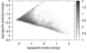
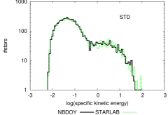
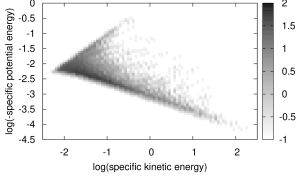
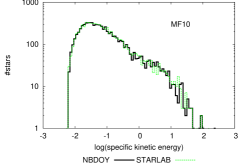
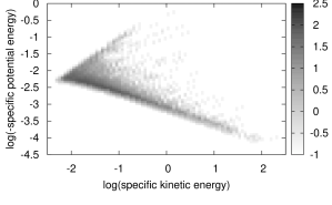
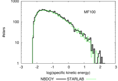
Figure 9: Specific kinetic and potential energy of escaping stars after 1000 N-body time units for standard setting (upper panels), MF10 runs (middle panels) and MF100 (lower panels). Left panels: Shown is the absolute number of stars in a given kinetic-vs.-potential energy bin (logarithmic bins) for starlab simulations (logarithmic grey scaling). Right panels: Comparison of kinetic energy distributions from nbody4 (black lines) and starlab simulations (green lines).

As a final check we compare the specific potential and kinetic energies of stars escaping the cluster, as especially their kinetic energies might sensitively depend on details in the treatment of binaries and close encounters in general.

To this end we determine for each star in each simulation its potential and kinetic energy from its position and velocity within the cluster, and divide by the mass of the star. We choose to compare only data at an age of 1000 N-body time units, hence sufficiently after core collapse. Results are presented in Fig. 9.

The left panels depict the distribution of kinetic versus potential energy from our starlab runs for the different mass function settings. A clear bifurcation is visible: the upper branch/edge consists of stars which are barely unbound (and a fraction of those might become recaptured by the cluster). With time these barely unbound stars migrate outwards in the cluster, into cluster regions with low specific potential energy (i.e. downwards in the left panels of Fig. 9). Stars with higher (specific) kinetic energy migrate faster, hence in the same time reach farther distances (i.e. regions characterised by lower specific potential energy). Core collapse is the earliest and by far strongest event leading to the unbinding of stars. Hence, the lower branches consist of stars which became unbound during core collapse, as they had the longest time to travel farthest. Stars in between the two main branches became unbound after core collapse.

There are two main mechanisms to accelerate stars sufficiently to become unbound: multiple weak encounters (“evaporating stars”) and single/few strong encounters (“ejected stars”, usually star-binary or binary-binary interactions). In the case of clusters with a stellar mass function, “ejected” stars can originate either i) from a scattering event of a single star on a binary (here the energy gain for the scattered star is small, as the energy gain originates from the shrinking binary orbit alone) or ii) from an exchange interaction (in this case the energy gain for the ejected star is large, as the energy gain originates from the orbit shrinking and the change in potential energy, as primarily a low-mass binary component is exchanged by a high-mass intruder star).

For an in-depth study of “evaporating” vs. “ejected” stars see Küpper et al. (2008). On average, “ejected” stars have higher kinetic energies than “evaporating” stars. Especially the stars with the highest kinetic energies are exclusively “ejected” stars. The maximum velocity gain a star can get during an interaction with a binary is of the order of the maximum orbital velocity of the binary stars. For an equal-mass binary the orbital velocity is directly related to the hardness of the binary, while for unequal-mass binaries the mass ratio between the binary stars plays the dominant role. The hardening of a binary is a long process. Hence, for equal-mass systems highly energetic ejected stars can only appear well after core collapse (and the formation of the first binaries), while for systems with a stellar mass function they can appear already right at core collapse. This effect is seen in Fig. 9, upper left panel: for the standard models, the lower branch shows a break at a specific kinetic energy $\sim$ -0.3, where stars with higher kinetic energy are slightly offset towards higher potential energies (i.e. closer to the cluster centre). This can be understood if these high-energy “ejected” stars left the cluster after the “evaporating” stars with lower kinetic energies (and therefore had less travel time), due to the time required for a sufficient hardening of the binaries.

The distinction into “evaporating” and “ejected” stars can also be seen in Fig. 9, upper right panel, which show a pronounced dip between these constituents. For systems with a stellar mass function, the contribution from “scattered” stars increases for wider mass functions, as the probability of a low-mass star being scattered at a high-mass binary increases. This increases the contribution of stars with intermediate kinetic energies, filling up the dip seen in Fig. 9, upper right panel. In addition, the “exchanged” stars can get up to higher kinetic energies for wider mass function, as the possible energy gain due to the change in potential energy increases. This is seen at the high-energy end of the distributions in Fig. 9, right panels.

We employ again a Kuiper test to test for statistically significant differences between the nbody4 and starlab energy distributions, both for the potential and the kinetic energy. For the standard and the MF10 runs we find no statistically significant deviations. For the MF100 runs, we find probabilities of 3.1% (kinetic energy) and 0.24% (potential energy), hence significant/highly significant deviations. Visual inspection shows that the energy distributions are slightly narrower for the starlab runs compared to the nbody4 results. With $\sim$10,000 stars in each sample, the Kuiper test gives a statistically significant difference. From a more detailed analysis of the binned distributions shown in Fig. 9, we find deviations between the two distributions of order $\la 2\sigma$ for $\sigma$ determined from the Poisson distributions which are expected to describe the number of stars in each bin.

9 Conclusions

We presented the first systematic in-depth study on how well results from the two major N-body codes nbody (here nbody4) and starlab are comparable. We started with three sets of input models (50 initial configurations each, for three different stellar mass functions) and evolved these input models independently with nbody4 and starlab. We analysed the results in a consistent way, and developed statistical tools to quantitatively compare the median results of a variety of parameters (for each stellar mass functions) derived using the two codes.

Overall, the agreement between the results obtained from the nbody4 runs and from the starlab runs is very good. Statistically significant deviations were only found for the energy conservation before core collapse (where nbody4 is significantly worse, likely due to problems at the interface between the main integrator and the KS algorithm for close encounter treatment) and for the kinetic/potential energy distributions of escaping stars in the MF100 runs (with the starlab distributions being slightly narrower).

While testing the binary eccentricity distributions against the common assumption of a thermal distribution, we find good agreement for the main simulations, both for starlab and nbody4. However, extending the number of test clusters (for starlab only), we find statistically significant biases towards higher eccentricities than a thermal distribution would predict. These deviations are driven by the dynamically least evolved binaries, while stars with probably the highest number of previous encounters tend to be more thermalised (though especially for the MF10 setting [i.e. a narrow mass range] statistically significant deviations remain for a number of subsets).

We tested our approach for biases, potentially induced by splitting the simulations into single snapshots and by the binary tree reconstruction. None of these effects result in statistically significant deviations.

In summary, we have shown that for purely dynamical N-body modelling results obtained from starlab and nbody4 are consistent with each other, allowing to combine these results without introducing systematic effects.

A similar study including stellar/binary evolution still needs to be performed.

10 Acknowledgements

PA acknowledges funding by NWO (grant 614.000.529) and the European Union (Marie Curie EIF grant MEIF-CT-2006-041108). We would like to thank the International Space Science Institute (ISSI) in Bern, Switzerland, where parts of the data were analysed and parts of this paper were written, for their hospitality and support. We would like to acknowledge the lively and stimulating discussions at the MoDeST-8 meeting in Bad Honnef (organized among others by Pavel Kroupa), especially with Sverre Aarseth and Peter Berczik, as well as with Andreas Küpper. PA would like to acknowledge fruitful technical discussions with Ines Brott and Evghenii Gaburov.

References

- Aarseth (1999) Aarseth, S. J. 1999, PASP, 111, 1333
- Aarseth (2003) Aarseth, S. J. 2003, Gravitational N-Body Simulations (Gravitational N-Body Simulations, by Sverre J. Aarseth, pp. 430. ISBN 0521432723. Cambridge, UK: Cambridge University Press, November 2003.)
- Anders (2008) Anders, P. 2008, et al. in prep.
- Baumgardt et al. (2006) Baumgardt, H., Gualandris, A., & Portegies Zwart, S. 2006, MNRAS, 372, 174
- Goodman et al. (1993) Goodman, J., Heggie, D. C., & Hut, P. 1993, ApJ, 415, 715
- Gualandris et al. (2005) Gualandris, A., Portegies Zwart, S., & Sipior, M. S. 2005, MNRAS, 363, 223
- Heggie (1975) Heggie, D. C. 1975, MNRAS, 173, 729
- Heggie (2001) Heggie, D. C. 2001, astro-ph/0110021
- Hurley et al. (2005) Hurley, J. R., Pols, O. R., Aarseth, S. J., & Tout, C. A. 2005, MNRAS, 363, 293
- Kuiper (1962) Kuiper, N. H. 1962, Proc. of the Koninklijke Nederlandse Akademie van Wetenschappen, Series A, 63, 38
- Küpper et al. (2008) Küpper, A. H. W., Kroupa, P., & Baumgardt, H. 2008, MNRAS, 389, 889
- Kustaanheimo & Stiefel (1965) Kustaanheimo, P. & Stiefel, E. 1965, J. Reine Angew. Mathe.
- Löckmann & Baumgardt (2008) Löckmann, U. & Baumgardt, H. 2008, MNRAS, 384, 323
- Makino (1991) Makino, J. 1991, ApJ, 369, 200
- Makino & Aarseth (1992) Makino, J. & Aarseth, S. J. 1992, PASJ, 44, 141
- Makino et al. (2003) Makino, J., Fukushige, T., Koga, M., & Namura, K. 2003, PASJ, 55, 1163
- Mikkola & Aarseth (1993) Mikkola, S. & Aarseth, S. J. 1993, Celestial Mechanics and Dynamical Astronomy, 57, 439
- Mikkola & Aarseth (1996) Mikkola, S. & Aarseth, S. J. 1996, Celestial Mechanics and Dynamical Astronomy, 64, 197
- Nitadori & Makino (2008) Nitadori, K. & Makino, J. 2008, New Astronomy, 13, 498
- Plummer (1911) Plummer, H. C. 1911, MNRAS, 71, 460
- Portegies Zwart et al. (2004) Portegies Zwart, S. F., Baumgardt, H., Hut, P., Makino, J., & McMillan, S. L. W. 2004, Nature, 428, 724
- Portegies Zwart et al. (2001) Portegies Zwart, S. F., McMillan, S. L. W., Hut, P., & Makino, J. 2001, MNRAS, 321, 199
- Portegies Zwart et al. (2007) Portegies Zwart, S. F., McMillan, S. L. W., & Makino, J. 2007, MNRAS, 374, 95
- Press et al. (1992) Press, W. H., Teukolsky, S. A., Vetterling, W. T., & Flannery, B. P. 1992, Numerical recipes in FORTRAN. The art of scientific computing (Cambridge: University Press, 2nd ed.)
- Salpeter (1955) Salpeter, E. E. 1955, ApJ, 121, 161
- van den Berk et al. (2007) van den Berk, J., Portegies Zwart, S. F., & McMillan, S. L. W. 2007, MNRAS, 379, 111
- Vesperini et al. (2003) Vesperini, E., Zepf, S. E., Kundu, A., & Ashman, K. M. 2003, ApJ, 593, 760