Markov Chain Monte Carlo Estimation of Quantum States

Abstract

We apply a Bayesian data analysis scheme known as the Markov Chain Monte Carlo (MCMC) to the tomographic reconstruction of quantum states. This method yields a vector, known as the Markov chain, which contains the full statistical information concerning all reconstruction parameters including their statistical correlations with no a priori assumptions as to the form of the distribution from which it has been obtained. From this vector can be derived, e. g. the marginal distributions and uncertainties of all model parameters and also of other quantities such as the purity of the reconstructed state. We demonstrate the utility of this scheme by reconstructing the Wigner function of phase-diffused squeezed states. These states posses non-Gaussian statistics and therefore represent a non-trivial case of tomographic reconstruction. We compare our results to those obtained through pure maximum-likelihood and Fisher information approaches.

I Introduction

The tomographic reconstruction of quantum states represents an important laboratory tool in both quantum optics and quantum information alike. It can be applied, for example, to the reconstruction of the dynamical interaction between quantum systems in a technique known as quantum process tomography. This latter technique is important in quantum computing, where the characterization of quantum gates is essential to the overall quantum circuit Chuang and Nielsen (1997); Poyatos et al. (1997); Lanyon et al. (2007). Tomography has even been used as part of the optimization of advanced interferometry as was done in the preparation of frequency dependent squeezing Chelkowski et al. (2005).

Since the theoretical discovery by Vogel and Risken Vogel and Risken (1989) that the Wigner function can be reconstructed from homodyne detector data, a number of reconstruction schemes have been developed ranging from direct inversion of the tomographic data by means of the filtered-back projection method Smithey et al. (1993) to statistical methods such as maximum-likelihood estimation Hradil (1997); Banaszek et al. (1999); Fiurášek (2001); Lvovsky (2004); Hradil et al. (2006); Řeháček et al. (2007). An important feature of maximum-likelihood methods is the guaranteed positive “semi-definiteness” of the reconstructed state. The result of a maximum-likelihood reconstruction method is either a density matrix Lvovsky (2004); Hradil et al. (2006) or a set of parameters D’Ariano et al. (2000); Ourjoumtsev et al. (2006) which have maximized the likelihood functional given a model of the measurement apparatus and of the parameterized state. A full analysis of the experimental data, however, should also answer important questions regarding error-bars on the estimation of the state parameters, possible correlations amongst the parameters, and error-propagation when using the reconstructed state for further calculations of quantities such as the purity of the state or amount of entanglement.

Several methods have been proposed in the literature to put error-bars on the reconstructed quantum states. For linear reconstruction techniques based on the averaging of sampling functions over the experimental data Welsch et al. one can calculate the statistical uncertainties of the estimated quantities by evaluating variances of the linear estimators Leonhardt et al. (1996). Another possible approach is to numerically simulate the whole measurement and reconstruction process many times assuming that the reconstructed state is the true state that is being measured upon. The error bars are then calculated from the resulting ensemble of reconstructed states D’Ariano et al. (1999). Finally, uncertainties on estimates obtained by maximum-likelihood method can be determined by evaluating the Fisher information matrix Řeháček et al. (2008). This latter approach essentially relies on approximation of the likelihood function by a Gaussian and becomes exact only asymptotically in the limit of a very large number of experimental data.

In the present paper we show that the uncertainties in quantum state estimation can be consistently determined by using a general and statistically well motivated Bayesian analysis scheme known as the Markov Chain Monte Carlo (MCMC). The method is based on the implementation of a Markov chain to search the parameter space resulting in a set of samples from the joint posterior probability density distribution on the unknown parameters of the model. This technique produces several important results. First, it yields the Markov chain containing all of the relevant statistical information about the parameter space. Second, one can extract a set of marginalized probability density distributions for each parameter quantifying the degree of uncertainty on their estimation. Third, the resulting chain can be used in further calculations, where one can produce probability density distributions on quantities such as of the purity or amount of entanglement of the reconstructed state.

This paper is divided into the following sections: in Sec. II the necessary concepts required from Bayesian data analysis are introduced and applied to the case of quantum state estimation. In Sec. III, the quantum likelihood function for phase-diffused squeezed states is derived. In Sec. IV the Markov chain Monte Carlo algorithm is introduced and finally in Sec. V both the technical details of the experimental realization as well as the results of the reconstruction are presented.

II Bayesian Data Analysis

Bayes’ Theorem prescribes the rule to invert the relationship between the experimental data already observed and the parameterized model which could have generated the measured data set. The theorem reads

$$p(\vec{\lambda}|D\,,I)=\frac{p(D|\vec{\lambda}\,,I)p(\vec{\lambda}|I)}{p(D|I)},$$ (1)

where we use $D$ to represent our data, $I$ to represent our prior information or model of the experiment and $\vec{\lambda}$ to represent a vector of model parameters. The quantity $p(\vec{\lambda}|D\,,I)$ is known as the posterior distribution, $p(D|\vec{\lambda}\,,I)$ is known as the likelihood function, $p(\vec{\lambda}|I)$ is the prior distribution and $p(D|I)$ is a normalization factor. The standard application of Bayesian analysis is to calculate the posterior distribution given a parameterized model of the sought after signal, the measured data and prior probability distributions on the values of the model parameters. These three elements are brought together through Eq. $\left(\ref{bayes_theorem}\right)$.

Let us now construct the likelihood function for the quantum estimation problem. A general measurement on a quantum system can be described by the so-called positive operator-valued measure (POVM). Each possible measurement outcome $j$ is associated with a POVM element $\Pi_{j}$ which is a positive semidefinite operator. The probability of outcome $j$ can be calculated as $P_{j}=\mathrm{Tr}[\Pi_{j}\rho(\vec{\lambda})]$ where $\rho(\vec{\lambda})$ denotes the density matrix of the measured quantum system that depends on the model parameters $\vec{\lambda}$. Since the total probability of some outcome is $1$, the POVM elements sum up to identity operator, $\sum_{j}\Pi_{j}=\openone$. This generic framework in particular encompasses a tomographic reconstruction of the state $\rho(\vec{\lambda})$ that consists of several different measurements $M$ with possible outcomes indexed by $l_{M}$. Then $j=(M,l_{M})$ becomes a multi-index indicating both the measurement setting and the measurement outcome for a given setting. Let $n_{j}$ denote the observed number of measurement outcome $j$ and $N=\sum_{j}n_{j}$ represents the total amount of collected data. The likelihood function $\mathcal{L}$ is the probability of observation of a particular set $\{n_{j}\}$ for a given $\vec{\lambda}$. It follows that $\mathcal{L}$ is given by a multinomial distribution and reads

$$\mathcal{L}=N!\prod_{j}^{N}\frac{P_{j}^{n_{j}}}{n_{j}!}.$$ (2)

In terms of the constituents of Bayes’s theorem the theoretical probabilities $\{P_{j}\}$ are functions of the parameters which are to be determined. The measured numbers of counts $\{n_{j}\}$ correspond to the data.

III The Likelihood Function for Phase-Diffused Squeezed States

The phase-diffused squeezed states were first introduced within the context of continuous-variable squeezing purification by Fiurášek et al. (2007); Franzen et al. (2006); Hage et al. (2006). They arise when squeezed states are transmitted over de-phasing quantum channels such as optical fibers affected by thermal fluctuations. These states are characterized by non-Gaussian statistics and therefore represent a non-trivial case for quantum state tomography.

The Wigner function for phase-diffused squeezed state is given by

$$W\left(x,p\right)=\frac{1}{2\pi\sqrt{V_{x}V_{p}}}\int_{-\infty}^{\infty}\!\!\exp{\left[-\left(\frac{x^{2}_{\phi}}{2V_{x}}+\frac{p^{2}_{\phi}}{2V_{p}}\right)\right]}\Phi\left(\phi\right)d\phi,$$ (3)

where $x_{\phi}=x\cos\phi+p\sin\phi$, $p_{\phi}=p\cos\phi-x\sin\phi$ with $x$ and $p$ as the standard position and phase quadratures and $\phi$ representing the random phase shifts distributed according to some probability distribution $\Phi\left(\phi\right)$. We use $V_{x}$ to represent the variance of the squeezed quadrature and $V_{p}$ for the variance of the anti-squeezed quadrature. We normalize the variances such that for vacuum state we have $V_{x}=V_{p}=1$ and the state is squeezed in $x$ quadrature if $V_{x}<1$. In the experiment we measure several different rotated quadratures $x_{\theta}$, where $\theta$ defines a specific measurement setting. The theoretical homodyne probability density distribution $p(x_{\theta})$ can be calculated from Wigner function as a marginal distribution. Integration of $W(x,p)$ over the conjugate quadrature $p_{\theta}$ yields, after some algebra

$$p\left(x_{\theta}\right)=\frac{1}{\sqrt{2\pi}}\int_{-\infty}^{\infty}\!\!\frac{1}{\sqrt{\tilde{V}(\phi)}}\exp{\left[-\frac{x_{\theta}^{2}}{2\tilde{V}(\phi)}\right]}\Phi\left(\phi-\theta\right)d\phi,$$ (4)

where $\tilde{V}(\phi)=V_{x}\cos^{2}\phi+V_{p}\sin^{2}\phi$.

The data from each measurement is binned into $L$ bins whose lower boundaries are defined by $Q_{\theta,l}$. The outer bins extend to infinity and we set $Q_{\theta,1}=-\infty$ and $Q_{\theta,L+1}=\infty$. The corresponding theoretical probability $P_{\theta,l}$ is given by integration of the probability density (4) over the bin,

$$P_{\theta,l}(\vec{\lambda})=\int_{Q_{\theta,l}}^{Q_{\theta,l+1}}p(x_{\theta})dx_{\theta}.$$ (5)

In our experiment, the results from two quadrature measurements were formed into histograms each containing a total of $L=70$ bins. From the perspective of direct data inversion this corresponds to an overdetermined system, because we need to estimate only three real parameters, c. f. below.

The POVM elements describing such binned homodyne detection can be expressed as

$$\Pi_{\theta,l}=\int_{Q_{\theta,l}}^{Q_{\theta,l+1}}|x_{\theta}\rangle\langle x_{\theta}|dx_{\theta},$$ (6)

where $|x_{\theta}\rangle$ is an eigenstate of quadrature operator $x_{\theta}$. Note that, by definition, the sum of theoretical probabilities over all bins is equal to one,

$$\sum_{l}P_{\theta,l}(\vec{\lambda})=1.$$ (7)

This is a mathematical expression of the fact that the homodyne detection always yields some outcome and, after each measurement, one of $n_{\theta,l}$ is increased by one. Put in a different way, the homodyne detection is described by a complete POVM (6) whose elements $\Pi_{\theta,l}$ satisfy the condition $\sum_{l}\Pi_{\theta,l}=\openone$.

Assuming the phase noise distribution, $\Phi\left(\phi\right)$, is a zero mean Gaussian, the state can be completely characterized by just three parameters $\vec{\lambda}=\{V_{x}\,,V_{p}\,,V_{\phi}\}$ where $V_{\phi}$ is the variance of the random phase shifts. The quantum log-likelihood function for the phase diffused squeezed states is finally obtained by taking the natural logarithm of Eq. $\left(\ref{qlikelihood}\right)$ giving us

$$\Lambda=\sum_{\theta,l}n_{\theta,l}\ln\left[P_{\theta,l}(\vec{\lambda})\right],$$ (8)

where, for simplicity, we ignore all terms that do not depend on the parameter values.

IV Markov Chain Monte Carlo Algorithm

The goal of our Bayesian reconstruction scheme is the calculation of marginalized posterior distributions on our model parameters ${\color[rgb]{0,0,0}\vec{\lambda}=\{V_{x},V_{p},V_{\phi}\}}$. To this end, the MCMC method can be used to generate samples drawn from the posterior distribution $p(\vec{\lambda}|D,I)$. Since this distribution is unknown one cannot directly sample from it and instead we sample from the distribution that is the product of the likelihood and the prior. The prior is chosen by considering the possible values of the parameters to be determined. Since the parameters to be determined in this case are variances, their values must be greater than zero. In order to assume relative ignorance in the value the parameters could take, we use a prior which only requires the variances to be positive and satisfy the Heisenberg uncertainty relation, $V_{x}V_{p}\geq 1$. Since the likelihood in this analysis is a sharply peaked function the choice of uniform priors has negligible effect on the numerical results of the MCMC . In this case Bayes’s theorem, Eq. $\left(\ref{bayes_theorem}\right)$, tells us that the likelihood function is proportional to the posterior distribution and since this is a function that we can compute for a given parameter space location we can use a standard sampling algorithm such as the Metropolis-Hastings sampler to draw from it. We describe our implementation of this sampler in Appendix A.

V Experimental Implementation

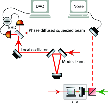
Figure 1: (Color online) Experimental setup: The experimental setup consists of an optical parametric amplifier (OPA) for the generation of the squeezed vacuum states, a phase shifter to induce the random phase noise and a homodyne detector to measure the prepared state. The mode cleaner was used to increase the fringe contrast at the balanced homodyne detector.

V.1 Description of the Experiment

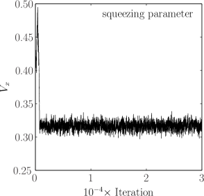
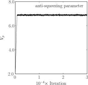
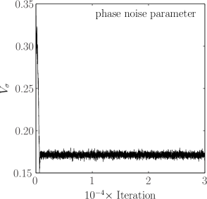
Figure 2: Markov chains: This figure depicts the evolution of the Markov chains where the abscissa represents the iteration number and the ordinate represents the value of the chain. After an initial “burn-in” period, in which the chains head to their steady-state positions, the chains eventually converge to a region of parameter space and begin to sample from the posterior distribution. The proposal distributions were taken to be Gaussian with the standard deviations $\Sigma_{x}=0.0042$, $\Sigma_{p}=0.022$, $\Sigma_{\phi}=0.0037$ corresponding to the squeezing parameter, the anti-squeezing parameter and the phase noise parameter, respectively. The starting values were randomly chosen with the only constraint that they be non-negative and obey $V_{x}V_{p}\geq 1$. The chains settled to their equilibrium positions with means of $\mu_{x}=0.316$, $\mu_{p}=6.888$, and $\mu_{\phi}=0.171$ corresponding to the squeezing, anti-squeezing and phase noise parameter respectively.

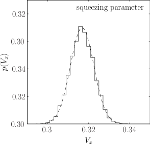
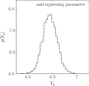
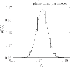
Figure 3: Marginalized posterior distributions: Each probability density was calculated using every tenth point from the marginalized chains corresponding to 38000 data points. The standard deviation of each density are $\sigma_{x}=0.0056$, $\sigma_{p}=0.0289$, and $\sigma_{\phi}=0.0020$ corresponding to the squeezing parameter, the anti-squeezing parameter and the phase noise parameter, respectively. The dotted line represents the result of the Fisher analysis.

Figure 1 shows the experimental setup that was used to prepare the phase diffused squeezed states. The full details of the setup are provided in Franzen et al. (2006) and will be summarized here. The squeezing source was an optical parametric amplifier (OPA) constructed from a type I non-critically phase-matched $\textrm{MgO:LiNbO}_{3}$ crystal inside a standing wave resonator, similar to the design that previously has been used in Chelkowski et al. (2007). The OPA was pumped with 50 mW of green light at 532 nm resulting in a classical gain of about 11. The length of the OPA cavity as well as the phase of the second harmonic pump beam were controlled using radio-frequency modulation/demodulation techniques. The mode cleaner was operated in high finesse mode $\mathcal{F}=10500$ resulting in a line width of 55 kHz. A non-classical noise power reduction of slightly more than 5.0 dB was directly observed with a homodyne detector in combination with a spectrum analyzer at a Fourier sideband frequency of 6.4 MHz.

The phase noise was induced by reflecting the squeezed field from a piezo-electric transducer (PZT) mounted high-reflection mirror that was quasi-randomly moved. The voltages applied to the PZTs were produced as follows. An independent random number generator produced data strings with a Gaussian distribution. The strings were digitally filtered to limit the frequency band to 2–2.5 kHz. The output interface was a common PC sound card with SNR of -110 dB. The sound volume was set to meet the desired standard deviation of channel phase noise.

Homodyne detection confirmed that the squeezing degraded in the same way when phase noise was increased. The detector difference currents were electronically mixed with a 6.4 MHz local oscillator. The demodulated signals were then filtered with a 400 kHz bandwidth low-pass filter and sampled with one million samples per second and 14 bit resolution using a National Instruments analog-digital sampling card.

V.2 Results of the MCMC

Figure 2 depicts the resulting chains after 40,000 iterations of the MCMC algorithm. The abscissa represents the number of iterations of the MCMC whereas the ordinate represents the parameter values. After an initial “burn-in” period of approximately 1000 iterations, in which the chain heads towards equilibrium, the chain converges and begins to sample from the posterior distribution (which in this Gaussian case also includes the region of maximum-likelihood). The development of criteria for the determination of chain convergence is a general problem which has been the subject of much research Brooks and Gelman (1998); El Adlouni et al. (2006). The general idea is to run multiple chains per estimation parameter and monitor their evolution both within each change and across each change. Convergence is inferred if all chains behave consistently. With respect to the case at hand, convergence of the chain can be inferred by comparing the locations to which the marginalized parameter chains have settled with the independent measurement of the $V_{x}$, and $V_{p}$ parameter values performed with a spectrum analyzer. In the absence of such an independent measurement, the criteria in Brooks and Gelman (1998); El Adlouni et al. (2006) can be used to infer convergence.

The width of the marginalized chains, i. e., their standard deviations, quantify the degree of uncertainty on the value of each parameter. By forming histograms of the chain as a function of each of the parameters we obtain their marginalized posterior probability distributions as shown in Fig. 3. From these posteriors we obtain the following uncertainties on the model parameters: $\sigma_{x}=0.0056$ for the squeezing parameter, $\sigma_{p}=0.0289$ for the anti-squeezing parameter and finally $\sigma_{\phi}=0.0020$ for the phase noise parameter. The proposal distributions, from which the posterior distribution samples have been drawn, were chosen to be Gaussians with the following standard deviations ${\color[rgb]{0,0,0}\Sigma_{x}}=0.0042$, ${\color[rgb]{0,0,0}\Sigma_{p}}=0.022$, ${\color[rgb]{0,0,0}\Sigma_{\phi}}=0.0037$ corresponding to the squeezing parameter, anti-squeezing parameter and phase noise parameter, respectively. These values were obtained through manual tuning of the MCMC algorithm. This is done by adjusting the individual standard deviations, i. e.  $\Sigma_{x}$, $\Sigma_{p}$, $\Sigma_{\phi}$, until the proportion of accepted jumps reaches approximately $44\%$ Gelman et al. (2004).

As an independent test of the posterior standard deviations, we also calculated the Fisher information matrix Fisher (1925); Vallisneri (2008) given by

$$\mathcal{F}_{ij}=\left\langle\frac{\partial\Lambda}{\partial\lambda^{i}}\frac{\partial\Lambda}{\partial\lambda^{j}}\right\rangle.$$ (9)

The inverse Fisher matrix represents the covariance of the posterior probability distribution for the true parameters $\vec{\lambda}$ as inferred from a single experiment assuming Gaussian noise and constant priors over the parameter range of interest. The calculated standard deviations from the Fisher matrix are presented in Fig. 3 as well as in Table 1 where very good agreement is readily seen. It should be stressed that the posterior distribution standard deviations obtained from the Fisher matrix are only valid when assuming Gaussian noise whereas the posterior distribution standard deviations obtained from the Markov chain is valid regardless of the form of the posterior distribution. The results of the MCMC as well as of the Fisher analysis are compared in Table 1.

Figure 4 depicts the evolution of the log-likelihood function (Eq. (8)) for each iteration of the MCMC. It is seen that as the chains evolve through the “burn-in” stage the log-likelihood quickly increases. After approximately $1000$ iterations it has reached equilibrium whereupon parameter space jumps to higher likelihood values are balanced by jumps to lower likelihood values.

Figure 5 represents the spectrum of the squeezed state before the phase diffusion. The measured state is seen to have a squeezing strength of -4.98 dB or a variance of $V_{x}=0.31$ and an anti-squeezing strength of 8.39 dB or a variance of $V_{p}=6.91$. These values have not been corrected for dark noise and were measured using a video bandwidth (VBW) of 10.0 Hz, a resolution bandwidth (RBW) of 100 kHz and a sweep time (SWT) of 1.5 s. These values lie within the width of the respective posterior distributions obtained from the MCMC analysis. Furthermore, only two quadrature measurements, each containing just $100,000$ data samples, were required to obtain these results. This represents a significant savings in terms of experimental effort to reconstruct a non-Gaussian state.

Table 1: Standard deviations of posterior distributions: This table compares the standard deviations of the parameter posterior distributions obtained from the Markov chain Monte Carlo method and from the Fisher information matrix. The standard deviations represent the error on the estimation of the parameter values. The Fisher matrix returns the actual standard deviations only in the case of Gaussian noise.

	Parameter Estimates		Uncertainties
Parameter	MCMC	Maximum Likelihood	MCMC	Fisher
$V_{x}$	0.316	0.317	0.0056	0.0055
$V_{p}$	6.889	6.880	0.0289	0.0294
$V_{\phi}$	0.171	0.171	0.0020	0.0020

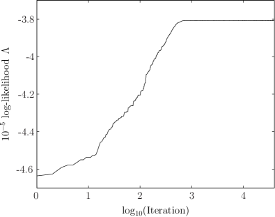
Figure 4: Log-Likelihood: Evolution of the log-likelihood as a function of iteration. The abscissa represents the iteration number and the ordinate the log-likelihood value. After approximately 1000 iterations the log-likelihood appears to have attained it’s maximum value at which point the chains have reached equilibrium and are sampling from the posterior distribution.

We also compare our results with that of a pure maximum-likelihood approach. This was achieved by altering step 3(d) of the Metroplis-Hastings sampler (see Appendix A) such that the chain remains at its current position whenever the likelihood ratio $r$ is less than one. This forces the chain to only move to regions of higher likelihood and hence quickly converge on the true maximum-likelihood location. The parameter values obtained at the maximum-likelihood were: $\hat{V}_{x}=0.317$ for the squeezing parameter, $\hat{V}_{p}=6.880$ for the anti-squeezing parameter and $\hat{V}_{\phi}=0.171$ for the phase noise parameter. These are, however, the only results obtained from the maximum-likelihood estimation alone. Since the MCMC chain contains a complete statistical description of the parameters, the statistical error on the reconstruction of both the quantum state itself as well as derived quantities from it, e. g. purity, can be exactly determined. This will be illustrated in the next section.

V.3 Reconstruction of the Quantum State

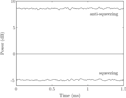
Figure 5: Zero span measurement of squeezing and anti-squeezing: The recorded amount of squeezing and anti-squeezing as measured by a balanced homodyne detector and spectrum analyzer at a Fourier frequency of 6.5 MHz. It is seen that approximately -4.98 dB of squeezing and 8.39 dB of anti-squeezing were directly measured without dark noise correction. These correspond to variances of $V_{x}=0.31$ and $V_{p}=6.91$, respectively. The units of the vacuum have been set to 1 corresponding to 0 dB.

Having completely characterized the parameter space, the final state can be reconstructed. In order to generate the Wigner function shown in Fig. 6, the Markov chain together with Eq. (3) were used to calculate the average Wigner function. The characteristic non-Gaussian statistics of the phase-space Wigner distribution is clearly manifested in the reconstructed state. It should be stressed that this averaging already takes into account the standard deviation of each value of the Wigner function since the parameter values are taken from the posterior distribution.

In addition to generating a phase-space plot of the reconstructed quantum state, the Markov chain can be used in further calculations of such properties as the purity of the reconstructed state. Figure 7 depicts such a result. Using the analytical definition of the purity

$$\mu=4\pi\int\!\!\!\int\!\!W^{2}\left(x\,,p\right)\,dxdp,$$ (10)

and the resulting chain from the MCMC, the purity can be calculated, automatically taking into consideration the statistical error and correlation on the parameters determined by the MCMC. The result is a probability density whose standard deviation quantifies the degree of uncertainty on the estimation of the purity. For the state in question, we obtain a purity of $\mu=0.5649\pm 0.0028$. It is important to note that this information is delivered directly from the MCMC itself; no additional assumptions as to the distribution of the errors and their correlation properties need to be made. Additionally, any one-dimensional quantity can be calculated in this manner. For example, if estimating the amount of entanglement of a non-Gaussian state, the logarithmic negativity Vidal and Werner (2002) can be calculated over the span of the resulting chain. The result will be a probability density quantifying the uncertainty on its value.

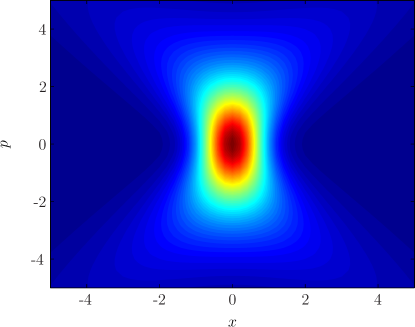
Figure 6: (Color Online) Reconstructed Wigner function: The Wigner function of the measured state as reconstructed using Eq. (3) and the Markov chain. This reconstruction contains all the relevant statistical information.

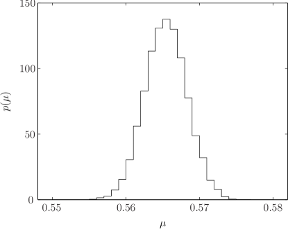
Figure 7: Reconstructed purity posterior distribution: The purity was calculated using the resulting Markov chain of 38,000 parameter values and Eq. $\left(\ref{purityformula}\right)$. This results in a probability density function which exactly quantifies the uncertainty on the estimation of the purity. The purity is calculated to be $\mu=0.5649\pm 0.0028$. No such result is possible with a pure maximum-likelihood approach.

VI Conclusion

We have applied a Bayesian data analysis scheme known as Markov chain Monte Carlo (MCMC) to the tomographic reconstruction of quantum states. Taking phase diffused squeezed states as an example, we have provided the details as to the derivation of the likelihood function as well as to the numerical implementation of the MCMC. The results include a set of probability density distributions which exactly quantify the degree of uncertainty on the estimation of the parameters. These results were compared to both a pure maximum-likelihood and a Fisher information approach. Furthermore, using the Markov chain in the calculation of the state’s purity enabled the construction of a probability density distribution on the value of the purity, thereby quantifying the degree of uncertainty on its calculation.

We note that MCMC scheme is completely general and can be applied to higher dimensional problems, such as the reconstruction of the density matrix, and will be the topic of future publications.

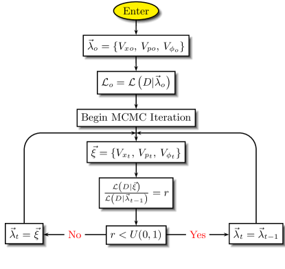
Figure 8: (Color online) MCMC program flow chart: A schematic explanation of the process of selecting MCMC samples from the posterior distribution. The lower loop iterates until the chain has converged to its equilibrium position and begins to sample from this posterior distribution.

Appendix A Metroplis-Hastings Sampler

Our implementation of the MCMC is based on the Metroplis-Hastings sampler. It is defined by performing the following steps (see also Fig. 8):

1. Generate initial values for parameters, $\vec{\lambda}_{o}$

2. Compute the quantity $\mathcal{L}_{0}=\mathcal{L}(D|\vec{\lambda}_{0})$

3. Iterate the following over the index $t$ until the chain has converged

   1. Generate a trial parameter vector $\vec{\xi}$ according to a proposal distribution $q(\vec{\lambda}_{t-1})$

   2. Compute the quantity $\mathcal{L}_{t}=\mathcal{L}(D|\vec{\xi})$. If $V_{x}V_{p}<1$ or some $V_{j}<0$ then set $\mathcal{L}_{t}=0$.

   3. Compute the ratio $r=\mathcal{L}_{t}/\mathcal{L}_{t-1}$

   4. Sample from a uniform distribution, $U(0\,,1)$
      if $\left\{\begin{array}[]{cclr}r>U,&\mathrm{set}&\vec{\lambda}_{t}=\vec{\xi},\,\mathcal{L}_{t}=\mathcal{L}&\mathrm{accepted}\\ r<U,&\mathrm{set}&\vec{\lambda}_{t}=\vec{\lambda}_{t-1},\,\mathcal{L}_{t}=\mathcal{L}_{t-1}&\mathrm{rejected}\end{array}\right.$

The proposal distribution $q(\vec{\lambda})$ used in stage 3(a) is used to select trial parameter values within the MCMC. Theoretically $q$ can be any distribution, however in practice it is sensible for the proposal distribution to suggest jumps that are local to the current location but large enough to allow an efficient exploration of the parameter space . Stage 3(b) ensures that the sampling is restricted to subspace of physically admissible values of parameters $\vec{\lambda}$. The simple difference between this MCMC method compared to that of a pure maximum-likelihood method is that for repeated stages within the Metropolis-Hastings sampler the chain has finite probability of jumping both to higher or lower values of likelihood.

References

- Chuang and Nielsen (1997) I. L. Chuang and M. A. Nielsen, J. Mod. Opt. 44, 2455 (1997).
- Poyatos et al. (1997) J. F. Poyatos, J. I. Cirac, and P. Zoller, Phys. Rev. Lett. 78, 390 (1997).
- Lanyon et al. (2007) B. P. Lanyon, T. J. Weinhold, N. K. Langford, M. Barbieri, D. F. V. James, A. Gilchrist, and A. G. White, Phys. Rev. Lett 99, 250505 (2007).
- Chelkowski et al. (2005) S. Chelkowski, H. Vahlbruch, B. Hage, A. Franzen, N. Lastzka, K. Danzmann, and R. Schnabel, Phys. Rev. A. 71, 013806 (2005).
- Vogel and Risken (1989) K. Vogel and H. Risken, Phys. Rev. A. 40, 2847 (1989).
- Smithey et al. (1993) D. T. Smithey, M. Beck, M. G. Raymer, and A. Faridani, Phys. Rev. Lett 70, 1244 (1993).
- Hradil (1997) Z. Hradil, Phys. Rev. A 55, 1561(R) (1997).
- Banaszek et al. (1999) K. Banaszek, G. M. D’Ariano, A. Paris, and M. F. Sacchi, Phys. Rev. A 61, 010304(R) (1999).
- Fiurášek (2001) J. Fiurášek, Phys. Rev. A 64, 024102 (2001).
- Lvovsky (2004) A. I. Lvovsky, J. Opt. B 6, S556 (2004).
- Hradil et al. (2006) Z. Hradil, D. Mogilevtsev, and J. Řeháček, Phys. Rev. Lett. 96, 230401 (2006).
- Řeháček et al. (2007) J. Řeháček, Z. Hradil, E. Knill, and A. I. Lvovsky, Phys. Rev. A 75, 042108 (2007).
- D’Ariano et al. (2000) G. M. D’Ariano, M. G. Paris, and M. F. Sacchi, Phys. Rev. A. 62, 023815 (2000).
- Ourjoumtsev et al. (2006) A. Ourjoumtsev, R. Tualle-Brouri, and P. Grangier, Phys. Rev. Lett. 96, 213601 (2006).
- (15) D. G. Welsch, W. Vogel, and T.Opatrný, Homodyne detection and quantum-state reconstruction, in Progress in Optics Vol. 39, edited by E. Wolf (Elsevier, Amsterdam,1999.).
- Leonhardt et al. (1996) U. Leonhardt, M. Munroe, T. Kiss, T. Richter, and M. G. Raymer, Opt. Commun 127, 144 (1996).
- D’Ariano et al. (1999) G. M. D’Ariano, M. F. Sacchi, and P. Kumar, Phys. Rev. A 61, 043022 (1999).
- Řeháček et al. (2008) J. Řeháček, D. Mogilevtsev, and Z. Hradil, New J. Phys. 10, 043022 (2008).
- Fiurášek et al. (2007) J. Fiurášek, P. Marek, R. Filip, and R. Schnabel, Phys. Rev. A 75, 050302(R) (2007).
- Franzen et al. (2006) A. Franzen, B. Hage, J. DiGuglielmo, J. Fiurášek, and R. Schnabel, Phys. Rev. Lett. 97, 150505 (2006).
- Hage et al. (2006) B. Hage, A. Franzen, J. DiGuglielmo, P. Marek, J. Fiurášek, and R. Schnabel, New. Jour. Phys. 9, 227 (2006).
- Chelkowski et al. (2007) S. Chelkowski, H. Vahlbruch, K. Danzmann, and R. Schnabel, Phys. Rev. A. 75, 043814 (2007).
- Brooks and Gelman (1998) S. P. Brooks and A. Gelman, Journal of Computational and Graphical Statistics 7, 434 (1998).
- El Adlouni et al. (2006) S. El Adlouni, A.-C. Favre, and B. Bobée, Computational Statistics & Data Analysis 50, 2685 (2006).
- Gelman et al. (2004) A. Gelman, J. B. Carlin, H. S. Stern, and D. B. Rubin, Bayesian data analysis (Chapman and Hall/ CRC, 2004), 2nd ed.
- Fisher (1925) R. A. Fisher, Proceedings of the Cambridge Philosophical Society 22, 700 (1925).
- Vallisneri (2008) M. Vallisneri, Phys. Rev. D. 77, 042001 (2008).
- Vidal and Werner (2002) G. Vidal and R. F. Werner, Phys. Rev. A 65, 032314 (2002).