Formation of Cooper pairs in quantum oscillations of electrons in plasma

Abstract

We study low energy quantum oscillations of electron gas in plasma. It is shown that two electrons participating in these oscillations acquire additional negative energy when they interact by means of a virtual plasmon. The additional energy leads to the formation a Cooper pair and possible existence of the superconducting phase in the system. We suggest that this mechanism supports slowly damping oscillations of electrons without any energy supply. Basing on our model we put forward the hypothesis the superconductivity can occur in a low energy ball lightning.

I Introduction

In the majority of cases plasma contains a great deal of electrically charged particles. Free electrons in metals can be treated as a degenerate plasma. If the motion of charged particles in plasma is organized, one can expect the existence of macroscopic quantum effects. For instance, collective oscillations of the crystal lattice ions can be exited in metals. These oscillations are interpreted as quasi-particles or phonons. Phonons are known to be bosons. The exchange of a phonon causes the effective attraction between two free electrons in plasma of metals. This phenomenon is known as the formation of a Cooper pair Coo56 and is important in the explanation of the superconductivity of metals. Cooper pairs can exist during a macroscopic time resulting in an undamped electric current. Unfortunately the formation of Cooper pairs is possible only at very low temperatures. Nowadays there are a great deal of attempts to obtain a superconducting material at high temperatures Gin00 .

Without an external field, e.g. a magnetic field, the motion of electrons in plasma is stochastic. It results in rather short times of plasma recombination. The laboratory plasma at atmospheric pressure without an energy supply recombines during $\sim 10^{-3}\thinspace\text{s}$ Smi93 . That is why free oscillations of electrons in plasma, i.e. without any external source of energy, will attenuate rather fast. Therefore to form a Cooper pair in plasma one should create a highly structured electrons motion to overcome the thermal fluctuations of background charged particles. Nevertheless it is known that a plasmon superconductivity can appear Pas92 .

In Ref. Dvo we studied quantum oscillations of electron gas in plasma on the basis of the solutions to the non-linear Schrödinger equation. The spherically and axially symmetrical solutions to the Schrödinger equation were found in our works. We revealed that the densities of both electrons and positively charged ions have a tendency to increase in the geometrical center of the system. The found solutions belong to two types, low and high energy ones, depending on the branch in the dispersion relation (see also Sec. II). We put forward a hypothesis that a microdose nuclear fusion reactions can happen inside a high energy oscillating electron gas. This kind of reaction can provide the energy supply to feed the system. In our works we suggested that the obtained solutions can serve as a model of a high energy ball lightning. Note that the suggestion that nuclear reactions can take place inside a ball lightning was also put forward in Ref. nuclfus .

In the present work we study a low energy solution (see Sec. II) which is also presented in our model Dvo . As we mentioned above a non-structured plasma usually recombines during several milliseconds. It is the main difficulty in constructing of long-lived plasma structures. In a high energy solution internal nuclear fusion reactions could compensate the energy losses. We suggest that the mechanism, which prevents the decay of low energy oscillations of the electron gas, is based on the possible existence of the plasma superconductivity. In frames of our model we show that the interaction of two electrons, described by spherical waves, can be mediated by a virtual plasmon. For plasmon frequencies corresponding to the microwave range, this interaction results in the additional negative energy. Then it is found that for a low energy solution with the specific characteristic this negative energy results in the effective attraction. Therefore a Cooper pair of two electrons can be formed because the interacting electrons should have oppositely directed spins. Using this result it is possible to state that the friction occurring when electrons propagate through the background matter can be significantly reduced due to the superconductivity phenomenon. We also discuss the possible applications of our results for the description of the a low energy ball lightning. It should be noticed that the appearance of the superconductivity inside of a ball lightning was considered in Ref. supercondold .

This paper is organized as follows. In Sec. II we briefly outline our model of quantum oscillations of the electron gas which was elaborated in details in Ref. Dvo . Then in Sec. III we study the interaction of two electrons when they exchange a virtual plasmon and examine the conditions of the effective attraction appearance. In Sec. IV we summarize and discuss the obtained results.

II Brief description of the model

In Ref. Dvo we discussed the motion of an electron with the mass $m$ and the electric charge $e$ interacting with both background electrons and positively charged ions. The evolution of this system is described by the non-linear Schrödinger equation,

$$\mathrm{i}\hbar\frac{\partial\psi}{\partial t}=H_{0}\psi,\quad H_{0}=-\frac{\hbar^{2}}{2m}\nabla^{2}+U(|\psi|^{2}),$$ (1)

where

$$U(|\psi|^{2})=e^{2}\int\mathrm{d}^{3}\mathbf{r}^{\prime}\frac{1}{|\mathbf{r}-\mathbf{r}^{\prime}|}\{|\psi(\mathbf{r}^{\prime},t)|^{2}-n_{i}(\mathbf{r}^{\prime},t)\},$$ (2)

is the term which is responsible for the interaction of an electron with background matter which includes electrons and positively charged ions with the number density $n_{i}(\mathbf{r},t)$. In Eq. (1) the wave function is normalized on the number density of electrons, $|\psi(\mathbf{r},t)|^{2}=n_{e}(\mathbf{r},t)$.

Note that in Eq. (1) the $c$-number wave function $\psi=\psi(\mathbf{r},t)$ depends on the coordinates of a single electron. Generally in a many-body system this kind of approximation is valid for an operator wave function, i.e. when it is expressed in terms of creation or annihilation operators. In Ref. KuzMak99 it was shown that it is possible to rewrite an exact operator Schrödinger equation using $c$-number wave functions for a single particle. Of course, in this case a set of additional terms appears in a Hamiltonian. Usually we neglect these terms (see Ref. Dvo ).

The solution to Eqs. (1) and (2) can be presented in the following way:

$$\psi(\mathbf{r},t)=\psi_{0}+\delta\psi(\mathbf{r},t),\quad|\psi_{0}|^{2}=n_{0},$$ (3)

where $n_{0}$ is the density on the rim of system, i.e. at rather remote distance from the center. The perturbative wave function $\delta\psi(\mathbf{r},t)$ for the spherically symmetrical oscillations has the form (see Ref. Dvo ),

$$\delta\psi(\mathbf{r},t)=e^{-\mathrm{i}\omega t}\delta\psi_{k}(\mathbf{r}),\quad\delta\psi_{k}(\mathbf{r})=A_{k}\frac{\sin kr}{r},$$ (4)

where $A_{k}$ is the normalization coefficient.

The dispersion relation which couples the frequency of the oscillations $\omega$ and the quantum number $k$ reads

$$k^{2}_{\pm}=\frac{\omega m}{\hbar}\left[1\pm\left(1-4\frac{\omega_{p}^{2}}{\omega^{2}}\right)^{1/2}\right].$$ (5)

It is convenient to rewrite Eq. (5) in the new variables $x=\omega/\omega_{p}$ and $y=k\sqrt{\hbar/2\omega_{p}m}$. Now it is transformed into the form,

$$y_{\pm{}}^{2}=\frac{x}{2}\left[1\pm\left(1-\frac{4}{x^{2}}\right)^{1/2}\right].$$ (6)

We represent the functions $y_{\pm{}}$ versus $x$ on Fig. 1.

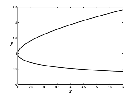
Figure 1: The dispersion relation for quantum oscillations of electron gas in plasma based on the results of Ref. Dvo .

One can see on Fig. 1 that there are two branches $y_{\pm{}}$ in the dispersion relation, upper and lower ones. It is possible to identify the upper branch with a high energy solution and the lower branch – with a low energy one.

Generally Eqs. (1) and (2) include the interaction of the considered electron with all other electrons in the system. However since we look for the solution in the pertubative form (3) and linearize these equations, the solution to Eqs. (4) and (5) describe the interactions of the considered electron only with background electrons, which correspond to the coordinate independent wave function $\psi_{0}$, rather than with electrons which participate in spherically symmetrical oscillations.

III Interaction of two electrons performing oscillations corresponding to the low energy branch

In this section we discuss the interaction between two electrons participating in spherically symmetrical oscillations. This interaction is supposed to be mediated by a plasmon field $\varphi$. To account for the electron interaction with a plasmon one has to include the additional term $e\varphi$ into the Hamiltonian $H_{0}$ in Eq. (1). We also admit that electron gas oscillations correspond to the lower branch $y_{-{}}$ in the dispersion relation (6), i.e. we are interested in the dynamics of a low energy solution.

A plasmon field distribution can be obtained directly from the Maxwell equation for the electric displacement field $\mathbf{D}$,

$$(\nabla\mathbf{D})=4\pi\rho,$$ (7)

where $\rho$ is the free charge density of electrons. As it was mentioned in Ref. Dvo the vector potential for spherically symmetrical oscillations can be put to zero $\mathbf{A}=0$. Therefore only longitudinal plasmons can exist. Presenting the potential $\varphi$ in the form of the Fourier integral,

$$\varphi(\mathbf{r},t)=\int\frac{\mathrm{d}\omega\mathrm{d}^{3}\mathbf{p}}{(2\pi)^{4}}\varphi(\mathbf{p},\omega)e^{-\mathrm{i}\omega t+\mathrm{i}\mathbf{p}\mathbf{r}},$$ (8)

we get the formal solution to Eq. (7) as

$$\varphi(\mathbf{r},t)=4\pi\int\mathrm{d}t^{\prime}\mathrm{d}^{3}\mathbf{r}^{\prime}G(\mathbf{r}-\mathbf{r}^{\prime},t-t^{\prime})\rho(\mathbf{r}^{\prime},t^{\prime}),$$ (9)

where

$$G(\mathbf{r},t)=\int\frac{\mathrm{d}\omega\mathrm{d}^{3}\mathbf{p}}{(2\pi)^{4}}\frac{1}{\mathbf{p}^{2}\varepsilon_{l}(\mathbf{p},\omega)}e^{-\mathrm{i}\omega t+\mathrm{i}\mathbf{p}\mathbf{r}},$$ (10)

is the Green function for the longitudinal plasmon. In Eq. (10) $\varepsilon_{l}$ stands for the longitudinal permittivity. Note that to choose the exact form of the Green function (10) one has to specify passing-by a residue at $\mathbf{p}=0$. We will regularize the Green function by putting a cut-off at small momenta. It should be noticed that the more rigorous derivation of the plasmon Green function is presented in Ref. plasmonprop .

To relate Eq. (9) with the distribution of electrons we can take that free charge density is proportional to the probability distribution, $\rho=e|\psi|^{2}$. Then, using Eq. (9) and the Schrödinger equation (1) with the new Hamiltonian $H=H_{0}+e\varphi$ we obtain the closed non-linear equation for the the electron wave function only.

Now we write down the new Hamiltonian explicitly,

$$H=H_{0}+V,\quad V=4\pi e^{2}\int\mathrm{d}t^{\prime}\mathrm{d}^{3}\mathbf{r}^{\prime}G(\mathbf{r}-\mathbf{r}^{\prime},t-t^{\prime})|\psi(\mathbf{r}^{\prime},t^{\prime})|^{2}.$$ (11)

As we mentioned in Sec. II the term $H_{0}$ describes the properties of a single electron including its interactions with background particles. The second term $V$ in the Hamiltonian (11) is responsible for the interactions between two separated electrons. The scattering of two electrons is due to this interaction.

It is possible to introduce the additional energy acquired in scattering of two electrons as

$$\Delta E=\langle\psi|V|\psi\rangle=4\pi e^{2}\int\mathrm{d}t^{\prime}\mathrm{d}^{3}\mathbf{r}^{\prime}\mathrm{d}t\mathrm{d}^{3}\mathbf{r}\psi^{*{}}(\mathbf{r},t)\psi^{*{}}(\mathbf{r}^{\prime},t^{\prime})G(\mathbf{r}-\mathbf{r}^{\prime},t-t^{\prime})\psi(\mathbf{r},t)\psi(\mathbf{r}^{\prime},t^{\prime}).$$ (12)

In Eq. (12) we add one additional integration over $t$ which is convenient for further calculations. To take into account the exchange effects one has to replace the products of the electrons wave functions in the integrand in Eq. (12) with the symmetric or antisymmetric combinations of the basis wave functions,

$$\psi(\mathbf{r},t)\psi(\mathbf{r}^{\prime},t^{\prime})\to \frac{1}{\sqrt{2}}[e^{-\mathrm{i}\omega_{1}t-\mathrm{i}\omega_{2}t^{\prime}}\psi_{k_{1}}(\mathbf{r})\psi_{k_{2}}(\mathbf{r}^{\prime})\pm e^{-\mathrm{i}\omega_{2}t-\mathrm{i}\omega_{1}t^{\prime}}\psi_{k_{2}}(\mathbf{r})\psi_{k_{1}}(\mathbf{r}^{\prime})],$$

$$\psi^{*{}}(\mathbf{r},t)\psi^{*{}}(\mathbf{r}^{\prime},t^{\prime})\to \frac{1}{\sqrt{2}}[e^{\mathrm{i}f_{1}t+\mathrm{i}f_{2}t^{\prime}}\psi_{q_{1}}^{*{}}(\mathbf{r})\psi_{q_{2}}^{*{}}(\mathbf{r}^{\prime})\pm e^{\mathrm{i}f_{2}t+\mathrm{i}f_{1}t^{\prime}}\psi_{q_{2}}^{*{}}(\mathbf{r})\psi_{q_{1}}^{*{}}(\mathbf{r}^{\prime})],$$ (13)

where $k_{1,2}$ and $q_{1,2}$ are the initial and final quantum numbers, and $\omega_{1,2}$ and $f_{1,2}$ are the initial and final frequencies of electron gas oscillations. Since the total wave function of two electrons, which also includes their spins, should be anti-symmetric, the coordinate wave functions in Eq. (III) which are symmetrical correspond to anti-parallel spins. For the same reasons the anti-symmetrical functions in Eq. (III) describe particles with parallel spin.

It is worth to mention that in calculating the additional scattering energy (12) electrons should be associated with the perturbative wave function (4) rather than with the total wave function (3). However we will keep the notation $\psi$ for an electron wave function to avoid cumbersome formulas. Using the basis wave functions (4), Eqs. (12) and (III) as well as the known value of the integral,

$$\int_{0}^{\infty}\frac{\mathrm{d}s}{s}\sin(ps)\sin(ks)\sin(qs)=\frac{\pi}{8}[\mathrm{sign}(p+k-q)+\mathrm{sign}(p+q-k)-\mathrm{sign}(p+k+q)-\mathrm{sign}(p-k-q)],$$ (14)

we obtain for the additional energy the following expression:

$$\Delta E= \delta(f_{1}+f_{2}-\omega_{1}-\omega_{2})A_{q_{1}}^{*{}}A_{q_{2}}^{*{}}A_{k_{1}}A_{k_{2}}\frac{e^{2}\pi^{4}}{16}\int_{0}^{\infty}\frac{\mathrm{d}p}{p^{2}}$$

$$\times\bigg{\{}\frac{1}{\varepsilon_{l}(p,f_{1}-\omega_{1})}[\mathrm{sign}(p+k_{1}-q_{1})+\mathrm{sign}(p+q_{1}-k_{1})$$

$$-\mathrm{sign}(p+k_{1}+q_{1})-\mathrm{sign}(p-k_{1}-q_{1})]\times[1\leftrightarrow 2]$$

$$\pm\frac{1}{\varepsilon_{l}(p,f_{2}-\omega_{1})}[\mathrm{sign}(p+k_{2}-q_{1})+\mathrm{sign}(p+q_{1}-k_{2})$$

$$-\mathrm{sign}(p+k_{2}+q_{1})-\mathrm{sign}(p-k_{2}-q_{1})]\times[1\leftrightarrow 2]\bigg{\}},$$ (15)

where the symbol $[1\leftrightarrow 2]$ stands for the terms similar to the terms preceding each of them but with all quantities with a subscript $1$ replaced with the corresponding quantities with a subscript $2$.

We suggest that electrons move towards each other before the collision and in the opposite directions after the collision, i.e. $k_{1}=-k_{2}=k$ and $q_{1}=-q_{2}=q$. In this situation the electrons occupy the lowest energy state (see, e.g., Ref. LifPit78p191 ). Taking into account that the frequencies and the coefficients $A_{k}$ are even functions of $k$ [see Eq. (5)] we rewrite the expression for the additional energy in the form,

$$\Delta E= \delta(f-\omega)|A_{q}|^{2}|A_{k}|^{2}\frac{e^{2}\pi^{4}}{16}\int_{0}^{\infty}\frac{\mathrm{d}p}{p^{2}}\frac{1}{\varepsilon_{l}(p,f-\omega)}$$

$$\times[\mathrm{sign}(p+k-q)+\mathrm{sign}(p+q-k)-\mathrm{sign}(p+k+q)-\mathrm{sign}(p-k-q)]^{2},$$ (16)

where $\omega=\omega_{1}=\omega_{2}$ and $f=f_{1}=f_{2}$. It is important to note that only symmetric wave functions from Eq. (III) contribute to Eq. (III). The anti-symmetric wave functions convert Eq. (III) to zero. It means that only electrons with oppositely directed spins contribute to the additional energy.

Now we should eliminate the energy conservation delta function. One can make it in a standard way, $\delta(f-\omega)\to\text{Time}/(2\pi)$, and then divide the whole expression on the observation time. Since the energy is concerned in the scattering one has two possibilities for the momenta, $k+q=0$ or $k-q=0$. We can choose, e.g., the latter case supposing that $k>0$. In this situation one has for $\Delta E$ the following expression:

$$\Delta E=|A_{k}|^{4}\frac{e^{2}\pi^{3}}{32}\int_{0}^{\infty}\frac{\mathrm{d}p}{p^{2}}\frac{1}{\varepsilon_{l}(p,0)}[1-\mathrm{sign}(p-2k)]^{2}.$$ (17)

Finally accounting for the step function in the integrand we can present the additional energy in the form,

$$\Delta E=|A_{k}|^{4}\frac{e^{2}\pi^{3}}{8}\int_{0}^{2k}\frac{\mathrm{d}p}{p^{2}}\frac{1}{\varepsilon_{l}(p,0)}.$$ (18)

Depending on the sign of the the additional energy one has either effective repulsion or effective attraction.

As we have found in Ref. Dvo the typical frequencies of electron gas oscillations in our problem $\sim 2\omega_{p}$, which is $\sim 10^{13}\thinspace\text{s}^{-1}$. Such frequencies lie deep inside the microwave region. The permittivity of plasma for this kind of situation has the following form (see, e.g., Ref. Gin60 ):

$$\varepsilon_{l}(\omega)=1-\frac{\omega_{p}^{2}}{\omega^{2}+\nu^{2}},$$ (19)

where $\nu$ is the transport collision frequency. In Eq. (19) we neglect the spatial dispersion. It is clear that in Eq. (18) one has to study the static limit, i.e. $\omega\to 0$. Supposing that the density of electrons is relatively high, i.e. $\omega_{p}\gg\nu$, one gets that the permittivity of plasma becomes negative and the interaction of two electrons results in the effective attraction.

Note that at the absence of spatial dispersion the integral is divergent on the lower limit. Such a divergence is analogous to the infrared divergence in quantum electrodynamics. We have to regularize it by the substitution $0\to 1/a_{D}$, where $a_{D}=\sqrt{4\pi e^{2}n_{e}/k_{B}T}$ is the Debye length and $T$ is the plasma temperature.

Besides the energy $\Delta E$, which is acquired in a collision, an electron also has its kinetic energy and the energy of the interaction with background charged particles. For the effective attraction to take place we should compare the additional negative energy with the eigenvalue of the operator $H_{0}$, which includes both kinetic term and interaction with other electrons and ions. We suggest that two electrons, which are involved in the scattering, move towards each other, i.e. $\omega_{1}=\omega_{2}=\omega$. Therefore, if we get that $2\hbar\omega+\Delta E<0$, the effective attraction takes place.

Calculating the integral in Eq. (18) one obtains the following inequality to be satisfied for the attraction to happen:

$$x<\frac{\xi^{2}\pi^{2}}{256\alpha}\frac{n_{0}\nu^{2}\hbar v}{m\omega_{p}^{4}}\frac{(y-\tilde{y})}{y^{5}},\quad\tilde{y}=\frac{1}{2}\sqrt{\frac{\hbar\omega_{p}}{2mv^{2}}},$$ (20)

where $v=\sqrt{k_{B}T/m}$ is the thermal velocity of background electrons in plasma and $k_{B}\approx 1.38\times 10^{-16}\thinspace\text{erg/K}$ is the Boltzmann constant. In Eq. (20) we use the variables $x$ and $y$ which were introduced in Sec. II. We also assume that $A_{k}^{2}=n_{c}/k^{2}$, where $n_{c}$ is the density in the central region [see Eq. (4)]. As it was predicted in our work Dvo , $n_{c}$ should have bigger values that the density on the rim of the system. We can also introduce two dimensionless parameters, $\xi$ and $\alpha$, to relate the density in the center, the density of free electrons, and the rim density: $n_{c}=\xi n_{0}$ and $n_{e}=\alpha n_{0}$.

We suppose that $\alpha\sim 0.1$. It is known (see, e.g., Ref. PEv3 ) that the number density of free electrons in a spark discharge is equal to $10^{16}-10^{18}\thinspace\text{cm}^{-3}$. Approximately the same electrons number densities are acquired in a streak lightning. If one takes the rim density equal to the Loschmidt constant $n_{0}=2.7\times 10^{19}\thinspace\text{cm}^{-3}$, we arrive to the maximal value of $\alpha\sim 0.1$. In this case mainly the collisions with neutral atoms would contribute to the transport collision frequency. One can approximate this quantity as $\nu\approx v\sigma n_{c}$, where $\sigma=\pi R^{2}$ is the characteristic collision cross section and $R\sim 10^{-8}\thinspace\text{cm}$ is the typical atomic radius. Note that the process in question happens in the center of the system. That is why we take the central number density $n_{c}$ in the expression for $\nu$.

Finally we receive the following inequality to be satisfied for the effective attraction between two electrons to take place:

$$x<K\frac{\tau^{3/2}\xi^{4}}{\alpha^{3}}\frac{1}{y^{5}}\left(y-y_{0}\frac{\alpha^{1/4}}{\tau^{1/2}}\right),\quad y_{0}=\frac{1}{2}\sqrt{\frac{\hbar\omega_{0}}{2mv_{0}^{2}}}\approx 0.63,$$

$$K=\frac{\pi^{2}}{256}\frac{\hbar n_{0}^{3}v_{0}^{3}\sigma^{2}}{m\omega_{0}^{4}}\approx 1.1\times 10^{-11},$$ (21)

where $\tau=T/T_{0}$. In Eq. (21) we take the reference temperature $T_{0}=700\thinspace\text{K}$. Now one calculates other reference quantities like $v_{0}$ and $\omega_{0}$ as $v_{0}=\sqrt{k_{B}T_{0}/m}\approx 10^{7}\thinspace\text{cm/s}$ and $\omega_{0}=\sqrt{4\pi e^{2}n_{0}/m}\approx 2.9\times 10^{14}\thinspace\text{s}^{-1}$.

As one can see on Fig. 1 [see also Eq. (6)] the parameter $y$ is always more than $1$ for the upper branch. It means that the inequality in Eq. (21) can never be satisfied. On the contrary, there is a possibility to implement the condition (21) for the lower branch on Fig. 1. It signifies the existence of the effective attraction between electrons.

On Fig. 2 we plot the allowed regions where the effective attraction happens.

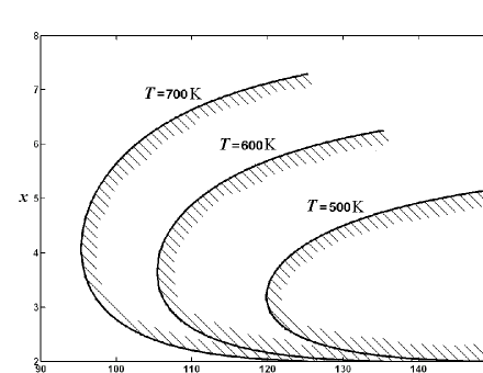
Figure 2: The allowed regions in the $(\xi,x)$ plane for the existence of the effective attraction between two electrons performing quantum oscillations corresponding to the lower branch on Fig. 1. We also add one more vertical axis on the right hand side demonstrating the behaviour of the quantum number $k$. Three zones for the temperatures $T=500\thinspace\text{K}$, $600\thinspace\text{K}$ and $700\thinspace\text{K}$ are shown here.

This plot was created for the constant value of $\alpha=0.1$. We analyze the condition (21) numerically. The calculation is terminated when we reach the point $x=2$. It has the physical sense since oscillations cannot exist for $x<2$ according to Eq. (6) (see also Fig. 1).

One can notice that always there is a critical value of the central density. It is equal to $120n_{0}$, $105n_{0}$ and $95n_{0}$ for the temperatures $T=500\thinspace\text{K}$, $600\thinspace\text{K}$ and $700\thinspace\text{K}$ respectively. It means that in the center of the system there is an additional pressure of about $100\thinspace\text{atm}$.

One has to verify the validity of the used approach checking that $y>\tilde{y}$ in Eq. (20). It would signify that that the the quantum number $k$ is more than $1/2a_{D}$. The values of $\tilde{y}$ are $0.42$, $0.38$ and $0.35$ for $T=500\thinspace\text{K}$, $600\thinspace\text{K}$ and $700\thinspace\text{K}$ respectively. Comparing these values with the curves on Fig. 2 one can see that the condition $y>\tilde{y}$ is always satisfied for all the allowed zone of the effective attraction existence.

For the effective attraction to happen one should have the negative values of $\varepsilon_{l}(0)$ in Eq. (18). Using Eq. (19) one can conclude that the following inequality should be satisfied: $\nu<\omega_{p}$ or equivalently $\xi<3.3\times 10^{3}\sqrt{\alpha/\tau}$. For $\alpha=0.1$ and temperatures $T=500\thinspace\text{K}$, $600\thinspace\text{K}$ and $700\thinspace\text{K}$ we get the critical values of $\xi$ as $1.2\times 10^{3}$, $1.1\times 10^{3}$ and $1.0\times 10^{3}$ respectively. One sees on Fig. 2 that all the curves lie far below the critical values of $\xi$. Therefore the condition $\varepsilon_{l}<0$ is always satisfied.

IV Summary and discussions

In conclusion we mention that we studied spherically symmetrical quantum oscillations of electron gas in plasma which correspond to a low energy solution to the Schrödinger equation Dvo . We suggested that two independent plasma excitations, corresponding to two separate electrons, can interact via exchange of a plasmon. Since the typical oscillations frequencies are very high and lie in the deep microwave region the plasma permittivity is negative and the interaction of two electrons result in the appearance of an attraction. For the this attraction to be actual we compared it with the kinetic energy of electrons and the energy of interaction of electrons with other background charged particles. The total energy of an electrons pair turned out to be negative for the lower branch in the dispersion relation (see Fig. 1 and Ref. Dvo ). Although we did not demonstrate it explicitly, using the same technique as in Sec. III one can check that the total energy of electrons is always positive for the upper branch. It means that even additional negative energy does not cause the attraction of electrons. It is interesting to mention that to obtain the master equations (1) and (2) in Ref. Dvo we neglected the exchange effects between an electron which corresponds to the wave function $\psi$ and the rest of background electrons (see also Ref. KuzMak99 ). This crude approximation is valid if the superconductivity takes place because in this case the friction, i.e. the interaction, between oscillating and background electrons is negligible.

The proposed plasmon superconductivity happening at spherically symmetrical oscillations of electrons could be implemented in a low energy ball lightning. Theoretical and experimental studies of ball lightnings have many years history (see, e.g., Ref. Tur98 ). This natural phenomenon, happening mainly during a thunderstorm, is very rare and we do not have so many its reliable witnesses. There were numerous attempts to generate in a laboratory stable structures similar to a ball lightning. Many theoretical models aiming to describe the observational data were put forward. In putting forward a ball lightning model one should try to explain these properties on the basis of the existing physical ideas without involvement of extraordinary concepts (see, e.g. Ref. Rab99 ) though they look very exciting. However none of the available models could explain all the specific properties of a fireball.

Among the existing ball lightning models one can mention the aerogel model Smi93 . According to this model fractal fibers of the aerogel can form a knot representing the skeleton of a ball lightning. Using this model it is possible to explain some of the ball lightning features. The interesting model of a ball lightning having complex onion-like structure with multiple different layers was put forward in Ref. Tur94 . However in this model an external source of electrical energy is necessary for a ball lightning to exist for a long time. The hypothesis that a ball lightning is composed of molecular clusters was described in Ref. Sta85 . This model can explain the existence of a low energy ball lightning. In Ref. RanSolTru00 the sophisticated ball lightning model was proposed, which is based on the non-trivial magnetic field configuration in the form of closed magnetic lines forming a knot. In frames of this model one can account for the relatively long life time of a ball lightning. It is worth to be noticed that though the properties of low energy fireballs can be accounted for within mentioned above models they are unlikely to explain its regular geometrical shape. The author of the present work has never observed a ball lightning, however according to the witnesses a fireball resembles a regular sphere. There are many other ball lightning models which are outlined in Ref. Smi88 .

The most interesting ball lightning properties are (see, e.g., Ref. Bar80 )

• There are both high and low energy ball lightnings. The energy of a low energy ball lightning can be below several hundred kJ. However the energy of a high energy one can be up to $1\thinspace\text{MJ}$.

• There are witnesses that a ball lightning can penetrate through a window glass. Sometimes it uses existing microscopic holes without destruction of the form of a ball lightning. It means that the actual size of a ball lightning is rather small and its visible size of several centimeters is caused by some secondary effects. Quite often a ball lightning can burn tiny holes inside materials like glass to pass through them. It signifies that the internal temperature and pressure are very high in the central region.

• A fireball is able to follow the electric field lines. It is the indirect indication that a ball lightning has electromagnetic nature, e.g., consists of plasma.

• A ball lightning has very long life-time, about several minutes. In Sec. I we mentioned that unstructured plasma without external energy source looses its energy and recombines extremely fast. If we rely on the plasma models of a ball lightning, it means that either there is an energy source inside of the system or plasma is structured and there exists a mechanism which prevents the friction in the electrons motion.

• In some cases there were reports that a ball lightning could produce rather strong electromagnetic radiation even in the X-ray range. It might signify that energetic processes, e.g. nuclear fusion reactions, can happen inside a fireball.

Quantum oscillations of electron gas in plasma Dvo can be a suitable model for a ball lightning. For example, it explains the existence of two types of ball lightnings, low and high energy ones. Our model accounts for the very small $\sim 10^{-7}\thinspace\text{cm}$ and dense central region as well as indirectly points out on the possible microdose nuclear fusion reactions inside of a high energy ball lightning.

In the present paper we suggested that superconductivity could support long life-time of a low energy fireball and described that this phenomenon could exist in frames of our model. It is unlikely that nuclear fusion reactions can take place inside a low energy ball lightning, i.e. this type of a ball lightning cannot have an internal energy source. Moreover as we mentioned in Ref. Dvo , electrons participating in spherically symmetrical oscillations cannot emit electromagnetic radiation. It means that the system does not loose the energy in the form of radiation. As a direct consequence of our model we get the regular spherical form of a fireball gratis. In Sec. III we made the numerical simulations for the temperature range $500-700\thinspace\text{K}$. According to the fireball witnesses Bar80 some low energy ball lightnings do not combust materials like paper, wood etc. The combustion temperature of these materials lie in the mentioned above range. It justifies our assumption.

Note the a ball lightning seems to be a many-sided phenomenon and we do not claim that our model explains all the existing electrical atmospheric phenomena which look like a ball lightning. However in our opinion a certain class of fireballs with the above listed properties is satisfactory accounted for within the model based on quantum oscillations of electron gas in plasma.

- (1) L. N. Cooper, Phys. Rev. 104, 1189 (1956).
- (2) V. L. Ginzburg, Phys. Usp. 43, 573 (2000).
- (3) B. M. Smirnov, Phys. Rep. 224, 1 (1993).
- (4) E. A. Pashitskiĭ, JETP Lett. 55, 333 (1992).
- (5) M. Dvornikov, S. Dvornikov, and G. Smirnov, Appl. Math. & Eng. Phys. 1, 9 (2001), physics/0203044; M. Dvornikov and S. Dvornikov, in Advances in plasma physics research, vol. 5, ed. by F. Gerard (Nova Science Publishers, Inc., 2007), pp. 197–212, physics/0306157.
- (6) M. D. Altschuler, L. L. House, and E. Hildner, Nature 228, 545 (1970); Yu. L. Ratis, Phys. Part. Nucl. Lett. 2, 64 (2005); the up-to-date discussion about nuclear fusion reactions as the energy source of a ball lightning is given in A. I. Nikitin, J. Russ. Laser Research 25, 169 (2004).
- (7) G. C. Dijkhuis, Nature 284, 150 (1980); M. I. Zelikin, J. Math. Sci. 151, 3473 (2008).
- (8) L. S. Kuz’menkov and S. G. Maksimov, Theor. Math. Phys. 118, 227 (1999).
- (9) E. M. Lifschitz, and L. P. Pitaevskiĭ, Statistical physics, Part II (Moscow, Nauka, 1978), pp. 370–376; for the more contemporary treatment see E. Braaten and D. Segel, Phys. Rev. D 48, 1478 (1993), hep-ph/9302213.
- (10) See p. 191 in Ref. plasmonprop .
- (11) V. L. Ginzburg, Propagation of electromagnetic waves in plasma (Moscow, Fizmatgiz, 1960), pp. 26–35.
- (12) B. M. Smirnov, in Physics encyclopedia, vol. 3, ed. by A. M. Prokhorov, (Moscow, Bolshaya Rossiĭskaya entsiklopediya, 1992), pp. 350–355.
- (13) D. J. Turner, Phys. Rep. 293, 1 (1998).
- (14) J. D. Barry, Ball lightning and bead lightning (Plenum Press, New York, 1980).
- (15) M. Rabinowitz, Astrophys. Space Sci. 262, 391 (1999), astro-ph/0212251.
- (16) D. J. Turner, Phil. Trans. R. Soc. Lon. A 347, 83 (1994).
- (17) I. P. Stakhanov, The physical nature of a ball lightning (Moscow, Energoatomizdat, 1985), 2nd ed., pp. 170–190.
- (18) A. F. Rañada, M. Soler, and J. L. Trueba, Phys. Rev. E 62, 7181 (2000).
- (19) B. M. Smirnov, The problem of a ball lightning (Moscow, Nauka, 1988), pp. 41–57.