Hydrodynamic relation in 2D Heisenberg antiferromagnet in a field

Abstract

The spin-stiffness $\rho_{s}$ of a 2D Heisenberg antiferromagnet depends non-analytically on external magnetic field. We demonstrate that the hydrodynamic relation between $\rho_{s}$, the uniform susceptibility $\chi$, and the spin-wave velocity $c$ is not violated by such a behavior because similar non-analytic terms from all three quantities mutually cancel out. In this work, explicit expressions for the field-dependent spin stiffness and for the magnon velocity of the 2D square lattice antiferromagnet are obtained by direct calculation to order $1/S$ and in the whole range of magnetic fields.

The effective description of spin-waves in the Heisenberg and easy-plane antiferromagnets by a hydrodynamic theory goes back to the work by Halperin and Hohenberg. HH Such a description implies the following hydrodynamic relation

$$\frac{\chi\,c^{2}}{\rho_{s}}=1,$$ (1)

between the susceptibility $\chi$, the spin-wave velocity $c$, and the spin stiffness $\rho_{s}$. The importance of an independent verification of such a relation using direct microscopic calculations has been recognized and received a significant attention in the past.Hamer Corresponding calculations confirming the validity of such a relation for the 2D square-lattice Heisenberg antiferromagnet (HAF) have been carried out in the early 1990s using the spin-wave theoryIgarashi ; Hamer to orders $1/S^{2}$ and $1/S^{3}$. Numerical studiesHuse_Singh ; Hamer ; Einarsson of the $S=1/2$ case of the same model have also given a strong support of the relation (1). While initial interest in this problem was motivated by the large-$J$ high-T_c materials, more recently, synthesis of small-$J$ quantum antiferromagnetsLandee has generated significant interest in the effects of external magnetic field in the properties of the HAFs, the regime that was previously unreachable.

Uniform magnetic field lowers the full rotational symmetry of the Heisenberg model to $O(2)$, making it equivalent to that of the the easy-plane antiferromagnets with the easy-plane of spin rotations perpendicular to the direction of the field. Note that the hydrodynamic consideration of Ref. HH, is also valid for the easy-plane antiferromagnets. Thus, at the first glance, it seems natural to assume that the two hydrodynamic descriptions should connect continuously. However, the situation is far less trivial as several quantities were shown to exhibit a non-analytic behavior in small fields. In the earlier work, Ref. Fisher_89, , field dependence of the ground-state energy and susceptibility was discussed for the non-linear ${\bm{\sigma}}$-model. The non-analytic field-dependent corrections have been found in the dimensions $D\leq 3$. A subsequent independent study, Ref. Zh_Nikuni, , obtained the same non-analytic behavior in small fields in the framework of the spin-wave theory. The recent work, Ref. Kopietz, , used a hybrid $1/S$-expansion$-{\bm{\sigma}}$-model approach to demonstrate that the spin-wave velocity in a 2D antiferromagnet also has a non-analytic dependence on the field, $c(H)-c(0)\propto|H|$ in the first $1/S$ order. Recent studies of the combined effects of the Dzyaloshinskii-Moriya and uniform magnetic field in the spectrum and the ground-state propertiesMila ; Chernyshev_05 of the 2D HAFs have also found non-analytic dependencies that are related to the ones discussed here.

The origin of the non-analytic behavior can be traced to the field-induced gap in one of the Goldstone modes. External field creates the so-called uniform-precession mode, which corresponds to the precession of the field-induced magnetization around the field direction with the energy equal to $H$. When the field is small, the mode is almost gapless and contributes to the fluctuation corrections to various quantities. These fluctuations may, potentially, induce non-hydrodynamic corrections in the corresponding $1/S$ order of the theory. Thus, the validity of the relation (1) in a field has to be verified.

In the case of the square-lattice HAF, out of three constants needed for the hydrodynamic relation it is only the spin stiffness for which the presence or absence of the non-analytic terms in the field-dependence remains unknown. In this work we carry out direct analytical calculations of $\rho_{s}$ to the necessary order in both $1/S$ and $H$ to: (i) identify such non-analytic terms, and (ii) verify that the non-analytic behavior of all three quantities does not lead to the violation of the hydrodynamic relation (1). In the course of such derivation, we also obtain an analytic expression for the spin stiffness to order $1/S$ and for all ranges of the field. In addition, the non-analytic behavior of the spin-wave velocity, previously obtained in Ref. Kopietz, by a hybrid $1/S-{\bm{\sigma}}$-model approach, is confirmed within the framework of the spin-wave theory and the compact analytic expression for the velocity renormalization is obtained for an arbitrary value of the field.

We would like to make a separate note on the recent work, Ref. Lauchli, , that combines a thorough numerical investigation of the static and dynamic properties of the $S=1/2$ square-lattice HAF in a field with the spin-wave analysis of the problem and provides a comprehensive comparison of the results. While in this work the spin stiffness is evaluated within the $1/S$ spin-wave approximation, it is done by numerical differentiation of the energy with respect to the twist angle, and no non-analytic behavior of $\rho_{s}$ vs. $H$ is discussed. Also, the hydrodynamic relation is used to provide a better estimate of the spin-wave velocity within the $1/S$ approach, but the validity of it is not verified.Lauchli

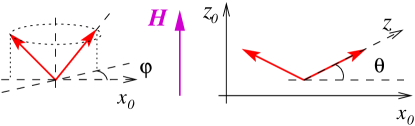
Figure 1: (Color online) Left: angle of twist $\varphi$ in the $x_{0}-y_{0}$ plane of spins in one sublattice with respect to the other. Right: field-induced canting by the angle $\theta$.

We consider the spin-$S$ HAF on the square lattice in an external field along the $z_{0}$ axis of the laboratory reference frame with the Hamiltonian given by

$$\hat{\cal H}=J\sum_{\langle ij\rangle}{\bf S}_{i}\cdot{\bf S}_{j}-H\sum_{i}S^{z_{0}}_{i}\ ,$$ (2)

where $\langle ij\rangle$ refer to the nearest-neighbor bonds. To study the spin stiffness, the Hamiltonian should be modified to introduce a twist angle between spins, rigidity to which should yields the stiffness directly. One of the prescriptionsHuse_Singh is to twist spins in every second row by the fixed angle $\varphi$. Another, intuitively more symmetric approach is to twist all the spins in one sublattice relative to the other.Lauchli In the latter method the twist energy is two times larger than in the former case because every spin has twice as many nearest neighbors that are twisted. For the Heisenberg model on a bi-partite lattice in zero field the direction of such a uniform twist is arbitrary. In the case of a non-zero external field, such a twist should be made in the plane perpendicular to the direction of the field, that is, in the $x_{0}-y_{0}$ plane, see Fig. 1. Thus, using the sublattice twist with a small angle $\varphi\ll 1$, the modified Hamiltonian reads:

$$\hat{\cal H}\approx J\sum_{\langle ij\rangle}{\bf S}_{i}\cdot{\bf S}_{j}-\frac{J\varphi^{2}}{2}\sum_{\langle ij\rangle}{\bf S}^{\perp}_{i}\cdot{\bf S}^{\perp}_{j}-H\sum_{i}S^{z_{0}}_{i}\ ,$$ (3)

where ${\bf S}^{\perp}_{i}=(S_{i}^{x_{0}},S_{i}^{y_{0}},0)$ and we have omitted the terms that are linear in $\varphi$, as they either vanish or contribute to the $\rho_{s}$-term only in the higher ($1/S^{2}$) order.Hamer ; Igarashi As such, the Hamiltonian (3) contains all the necessary terms to study both the classical limit of the model and the $1/S$ fluctuation corrections to it.

To study quantum fluctuations around the classical spin configuration it is convenient to transform spins to “rotating” local reference frames in which the quantization axis $z$ is along the classical spin direction.Zh_Nikuni ; field ; Chernyshev_06 Magnetic field cants spins toward its direction as is shown in Fig. 1. Assuming that the spins lie in the $x$–$z$ plane we perform transformation from the laboratory frame $(x_{0},z_{0})$ into the rotating frame $(x,z)$:Zh_Nikuni ; field

$$S_{i}^{z_{0}} = S_{i}^{z}\sin\theta-e^{i{\bf Q}r_{i}}S_{i}^{x}\cos\theta\ ,$$ (4)

$$S_{i}^{x_{0}} = e^{i{\bf Q}r_{i}}S_{i}^{z}\cos\theta+S_{i}^{x}\sin\theta\ ,\ \ S_{i}^{y_{0}}=S_{i}^{y}\ ,$$

where ${\bf Q}=(\pi,\pi)$ is the ordering wave-vector, and canting angle is as shown in Fig. 1. The spin Hamiltonian (3) in the local coordinate system (4) takes the form:

$$\hat{\cal H} \approx J\sum_{\langle ij\rangle}\Bigl{[}S_{i}^{y}S_{j}^{y}-\cos 2\theta\left(S^{z}_{i}S^{z}_{j}+S^{x}_{i}S^{x}_{j}\right)$$

$$\mbox{}-\frac{\varphi^{2}}{2}\left(S_{i}^{y}S_{j}^{y}+S^{x}_{i}S^{x}_{j}\sin^{2}\theta-S^{z}_{i}S^{z}_{j}\cos^{2}\theta\right)\Bigr{]}\,,$$

$$-H\sin\theta\sum_{i}S^{z}_{i}\ ,$$

where, again, the terms that are not contributing to the harmonic approximation are omitted.

At the first glance, the spin stiffness can be defined from the averaging of the second line in Eq. (Hydrodynamic relation in 2D Heisenberg antiferromagnet in a field) over the ground state. However, the situation is slightly more complex as the field-induced canting angle $\theta$, which should be found from the minimization of the classical energy in (Hydrodynamic relation in 2D Heisenberg antiferromagnet in a field),Zh_Nikuni also depends on the twist angle.Lauchli Performing such a minimization for (Hydrodynamic relation in 2D Heisenberg antiferromagnet in a field),Zh_Nikuni one obtains:

$$\sin\theta=h\left(1+\frac{\varphi^{2}}{4}\right),$$ (6)

where the terms of higher order in the twist angle are truncated and the dimensionless variable $h=H/(8JS)$, the field normalized to the saturation field $H_{s}=8JS$ at which spins become fully aligned, is introduced. With the help of (6) one can eliminate $\theta$ in (Hydrodynamic relation in 2D Heisenberg antiferromagnet in a field) to obtain

$$\hat{\cal H} \approx \hat{\cal H}_{\varphi=0}+\hat{\cal H}_{\rho_{s}}\ ,$$ (7)

where $\hat{\cal H}_{\varphi=0}$ contains no twist angle and $\hat{\cal H}_{\rho_{s}}$ is given by:

$$\hat{\cal H}_{\rho_{s}} = \frac{J\varphi^{2}}{2}\bigg{\{}\sum_{\langle ij\rangle}\Bigl{[}(1+h^{2})S_{i}^{z}S_{j}^{z}+h^{2}S^{x}_{i}S^{x}_{j}-S^{y}_{i}S^{y}_{j}\Bigr{]}$$ (8)

$${\phantom{\frac{J\varphi^{2}}{2}\sum_{\langle ij\rangle}}}-4Sh^{2}\sum_{i}S^{z}_{i}\bigg{\}}\ ,$$

The subsequent treatment of the Hamiltonian $\hat{\cal H}_{\varphi=0}$ involves standard bosonization of spin operators via the Holstein-Primakoff transformation to the first $1/S$ order:

$$S_{i}^{z}=S-a^{\dagger}_{i}a_{i}\ ,\ \ S_{i}^{-}\approx a^{\dagger}\sqrt{2S}\ ,\ \ S_{i}^{+}=(S_{i}^{-})^{\dagger}\ ,$$ (9)

which is followed by the Bogolyubov transformation.Zh_Nikuni This yields the linear spin-wave theory Hamiltonian:

$$\hat{\cal H}_{\varphi=0}\approx E_{\rm GS}+4JS\sum_{\bf k}\omega_{\bf k}\alpha^{\dagger}_{\bf k}\alpha_{\bf k}\ ,$$ (10)

see Ref. Zh_Nikuni, for details. The dimensionless frequency is:

$$\omega_{\bf k}=\sqrt{(1+\gamma_{\bf k})(1-(1-2h^{2})\gamma_{\bf k})}\ ,$$ (11)

and $\gamma_{\bf k}=(\cos k_{x}+\cos k_{y})/2$.

Figure 2: (Color online) $1/S$ quantum correction to the spin stiffness $-\delta\rho_{s}/JS$ as a function of the field $h$. Inset: $\rho_{s}/JS^{2}$ vs $h$ for $S=1/2$, dashed line is $\rho_{s}^{\rm cl}/JS^{2}$ vs $h$.

After diagonalization of $\hat{\cal H}_{\varphi=0}$, the spin stiffness can be found as a coefficient in front of $\varphi^{2}$ in the twist part $\hat{\cal H}_{\rho_{s}}$ of the Hamiltonian (8) by averaging the spin operators over the spin-wave ground state and keeping terms to $1/S$ order. Having in mind the extra factor of 2 in the sublattice twist approach, this finally yields:

$$\delta E_{\varphi}=\left\langle\hat{\cal H}_{\rho_{s}}\right\rangle=\varphi^{2}N\rho_{s}\ ,$$ (12)

where $\rho_{s}=\rho_{s}^{\rm cl}+\delta\rho_{s}$ with the classical and quantum contributions given by

$$\rho_{s}^{\rm cl} = JS^{2}\left(1-h^{2}\right)\ ,$$ (13)

$$\delta\rho_{s} = -JS\left[2n-\Delta(1+h^{2})+m(1-h^{2})\right]\ ,$$

where we use the following Hartree-Fock averages of the two-boson operator combinations:

$$n = \langle a^{\dagger}_{i}a_{i}\rangle=\frac{1}{2}\sum_{\bf q}\Bigl{[}\frac{1+h^{2}\gamma_{\bf q}}{\omega_{\bf q}}-1\Bigr{]}\ ,$$

$$\Delta = \langle a_{i}a_{j}\rangle=\frac{1}{2}(1-h^{2})\sum_{\bf q}\frac{\gamma_{\bf q}^{2}}{\omega_{\bf q}}\ ,$$ (14)

$$m = \langle a^{\dagger}_{i}a_{j}\rangle=\frac{1}{2}\sum_{\bf q}\frac{\gamma_{\bf q}+h^{2}\gamma_{\bf q}^{2}}{\omega_{\bf q}}\ ,$$

The above result (13) gives $\rho_{s}$ to the order $1/S$ and for the fields anywhere between zero and the saturation value. At $H=0$ the expression for $\rho_{s}$ in (13) and (Hydrodynamic relation in 2D Heisenberg antiferromagnet in a field) coincides with the known zero-field formula for the Heisenberg model. Igarashi ; Hamer The field-dependence of the quantum correction to the spin stiffness $\delta\rho_{s}$ is shown in Fig. 2. The inset presents $\rho_{s}$ for the spin-1/2 case. One of the interesting observations is that $\delta\rho_{s}$ changes sign as a function of the field. It also exhibits a singular behavior in the derivative as $h\rightarrow 1$, similar to the one discussed before for the magnetization,Zh_Nikuni and is related to the logarithmically vanishing scattering amplitude in the dilute 2D gas of bosons. The linear (non-analytic) field-dependence at small field is also clear from Fig. 2.

With the expressions (13) and (Hydrodynamic relation in 2D Heisenberg antiferromagnet in a field) at hand, one can now study the field dependence of $\rho_{s}$ at $h\rightarrow 0$. After some algebra one finds:

$$\rho_{s}=\rho_{s}^{H=0}-JS\sum_{\bf k}\left(\frac{1}{\omega_{\bf k}}-\frac{1}{\omega^{H=0}_{\bf k}}\right)+{\cal O}(h^{2}).$$ (15)

It is easy to see that due to the field-induced gap $\propto H$ in the magnon spectrum the fluctuation terms like the one in (15) are yielding corrections $\propto|H|$ in 2D. Some further algebra gives:

$$\rho_{s} = JS^{2}\left(Z_{\rho_{s}}+\frac{2}{\pi S}\,|h|\right)+{\cal O}(h^{2},1/S^{2})$$ (16)

$$\approx \rho_{s}^{H=0}\left(1+\frac{2}{\pi S}\,|h|\right),$$

where $\rho_{s}^{H=0}$ contains zero-field, $1/S$ renormalization factor $Z_{\rho_{s}}$, Ref. Hamer, , and the last expression is obtained within the same $1/S$ accuracy.

For completeness, we also list the corresponding $1/S$ expressions for the susceptibility. Magnetization of the square-lattice HAF is $M=M_{\rm cl}+\delta M$ with the classical part and the quantum correction given by:Zh_Nikuni

$$M_{\rm cl}=Sh,\ \ \ \ \delta M=-h(m+\Delta).$$ (17)

Using $\chi=\partial M/\partial H$ yields:

$$\chi=\chi_{\rm cl}+\delta\chi=\frac{1}{8J}\Bigl{[}1-\frac{1}{S}\bigl{(}m+\Delta-h^{2}I_{1}\bigr{)}\Bigr{]},$$ (18)

where $I_{1}$ stands for the integral

$$I_{1}=\sum_{\bf q}\frac{\gamma_{\bf q}^{2}(1+\gamma_{\bf q})^{2}}{\omega_{\bf q}^{3}}\ .$$ (19)

At small fields, the same algebra as above gives:

$$\chi = \frac{1}{8J}\Bigl{(}Z_{\chi}+\frac{4}{\pi S}\,|h|\Bigr{)}+{\cal O}(h^{2},1/S^{2})$$ (20)

$$\approx \chi^{H=0}\Bigl{(}1+\frac{4}{\pi S}\,|h|\Bigr{)}.$$

Figure 3 shows the field-dependence of the quantum correction to the susceptibility $\delta\chi$. The inset presents $\chi$ for the case of $S=1/2$. Similarly to $\delta\rho_{s}$, $\delta\chi$ changes sign as a function of the field. As is discussed in Ref. Zh_Nikuni, , $\chi$ has a singular logarithmic behavior at $h\rightarrow 1$ and the linear, non-analytic field-dependence at $h\rightarrow 0$ is also clearly seen in Fig. 3.

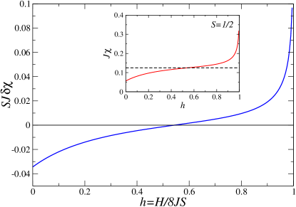
Figure 3: (Color online) $1/S$ quantum correction to the susceptibility $JS\delta\chi$ as a function of the field $h$. Inset: $J\chi$ vs $h$ for $S=1/2$, dashed line is $J\chi_{\rm cl}$.

For the square lattice HAF in external magnetic field the energy of magnons to the first-order of the $1/S$ expansion is given byfield

$$\bar{\varepsilon}_{\bf k}=4JS\omega_{\bf k}+\delta\varepsilon^{(1)}_{\bf k}+\delta\varepsilon^{(2)}_{\bf k}\ ,$$ (21)

where $\omega_{\bf k}$ is defined in Eq. (11), correction $\delta\varepsilon^{(1)}_{\bf k}$ includes the Hartree-Fock and the canting angle renormalizations

$$\delta\varepsilon^{(1)}_{\bf k} = \frac{4J}{\omega_{\bf k}}\Bigl{\{}\Delta\!-\!n\!+\!h^{2}(\Delta\!+\!m)\left[1-2\gamma_{\bf k}(1\!-\!h^{2})\right]$$

$$+ \gamma^{2}_{\bf k}\bigl{[}n-\Delta(1\!-\!h^{2}\!+\!2h^{4})-mh^{2}(3\!-\!2h^{2})\bigr{]}\Bigr{\}}$$

and $\delta\varepsilon^{(2)}_{\bf k}$ is the one-loop contributions from the three-magnon coupling:

$$\delta\varepsilon^{(2)}_{\bf k} = -4Jh^{2}(1-h^{2})$$

$$\times \sum_{\bf q}\biggl{[}\frac{\widetilde{\Gamma}_{1}({\bf k},{\bf q})^{2}}{\omega_{\bf q}\!+\omega_{\bf k-q+Q}\!-\omega_{\bf k}}+\frac{\widetilde{\Gamma}_{2}({\bf k},{\bf q})^{2}}{\omega_{\bf k}\!+\omega_{\bf q}\!+\omega_{\bf k+q-Q}}\biggr{]}$$

Explicit expressions for $\widetilde{\Gamma}_{1}({\bf k},{\bf q})$ and $\widetilde{\Gamma}_{2}({\bf k},{\bf q})$ are given in Ref. field, . After some algebra, the $1/S$ correction to the spin-wave velocity can be written as:

$$\frac{c-c_{0}}{c_{0}} = \frac{\Delta(1-h^{2}\!+h^{4})-n+mh^{2}(2-h^{2})}{S(1-h^{2})}$$

$$\mbox{}-\frac{h^{2}}{2S}\,I_{1}-\frac{2h^{2}}{S}\!\left.\biggl{(}\frac{I_{2}({\bf k})-4\Delta}{k^{2}}\biggr{)}\right|_{k\rightarrow 0}\ ,$$

where the bare spin-wave velocity is $c_{0}^{2}=8J^{2}S^{2}(1-h^{2})$ and the ${\bf k}$-dependent function in the last term is:

$$I_{2}({\bf k})=2(1-h^{2})\sum_{\bf q}\gamma_{1}\,\frac{\gamma_{1}\alpha_{1}\beta_{2}+\gamma_{2}\omega_{1}\omega_{2}}{\omega_{1}\omega_{2}(\omega_{1}+\omega_{2})}\ ,$$ (25)

with $\alpha_{1}=(1+\gamma_{1})$, $\beta_{2}=\left[1-(1-2h^{2})\gamma_{2}\right]$, and $1,2={\bf q},{\bf q-k}$.

The field-dependence of the quantum correction to the spin-wave velocity $\Delta c$, obtained by numerical evaluation of the integrals in Eq. (Hydrodynamic relation in 2D Heisenberg antiferromagnet in a field), is shown in Fig. 4. The inset presents the normalized magnon velocity for $S=1/2$. The linear (non-analytic) field-dependence at small field is clearly visible in Fig. 4. Behavior of $\Delta c$ at $h\rightarrow 1$ is also singular, similarly to other quantities. It is interesting to note that the correction to the spin-wave velocity $\Delta c$ is almost flat for $0.2\lesssim h\lesssim 0.9$.

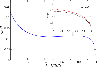
Figure 4: (Color online) $1/S$ quantum correction to the spin-wave velocity $\Delta c/J$ as a function of the field $h$. Inset: $c/2JS$ vs $h$ for $S=1/2$, dashed line is $c_{0}/2JS$ vs $h$.

It is easy to see that the first Hartree-Fock term in Eq. (Hydrodynamic relation in 2D Heisenberg antiferromagnet in a field) does not contribute to the anomalous non-analytic field dependence. After some more algebra, one can show that the same is true for the last term in (Hydrodynamic relation in 2D Heisenberg antiferromagnet in a field). The second term in Eq. (Hydrodynamic relation in 2D Heisenberg antiferromagnet in a field), on the other hand, yields at $h\rightarrow 0$:

$$\frac{\Delta c}{c_{0}}\approx-\frac{2h^{2}}{S}\sum_{\bf q}\left(\frac{1}{(\omega_{\bf q})^{3}}-\frac{1}{(\omega^{H=0}_{\bf q})^{3}}\right)=-\frac{|h|}{\pi S}\ .$$ (26)

This gives the same result as in Ref. Kopietz, :

$$c^{2}\approx c^{2}_{H=0}\left(1-\frac{2}{\pi S}\,|h|\right).$$ (27)

Combining the expressions for the small-field expansion of all three quantities, $\rho_{s}$, $\chi$, and $c$ from Eqs. (16), (20), and (27), one can easily see that the hydrodynamic relation (1) is obeyed as all the non-analytic terms explicitly cancel each other in the leading order in $h$. Moreover, such a verification of the relation (1) can be extended to an arbitrary field. Expanding the hydrodynamic relation (1) to $1/S$ order and observing that it is fulfilled at the classical level, $\chi_{\rm cl}\,c_{0}^{2}/\rho_{s}^{\rm cl}=1$, one concludes that for the hydrodynamic relation to exist the quantum corrections from all three quantities must cancel each other at any field in each order of $1/S$. For the $1/S$ corrections this leads to

$$\frac{\chi\,c^{2}}{\rho_{s}}-\frac{\chi_{\rm cl}\,c_{0}^{2}}{\rho_{s}^{\rm cl}}\approx\left(\frac{\delta\chi}{\chi_{\rm cl}}+2\frac{\Delta c}{c_{0}}-\frac{\delta\rho_{s}}{\rho_{s}^{\rm cl}}\right)=0\ .$$ (28)

Numerical verification of the above relation is made using expressions (13), (18), and (Hydrodynamic relation in 2D Heisenberg antiferromagnet in a field) and is presented by the solid line in Fig. 5. The dashed lines show contributions of individual terms in (28). One can conclude that the cancellation takes place for all values of $0<h<1$.

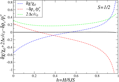
Figure 5: (Color online) Cancellation of the $1/S$ quantum corrections in the hydrodynamic relation (28) as a function of the field $h$ (solid line). Dashed lines show contributions of individual terms in (28).

Having in mind the relation (28), we can now obtain a much simpler expression for the spin-wave velocity renormalization in magnetic field:

$$\frac{c-c_{0}}{c_{0}}=\frac{1}{S}\Bigl{(}\frac{\Delta-n}{1-h^{2}}-\frac{h^{2}}{2}I_{1}\Bigr{)}\ ,$$ (29)

where $I_{1}$ is defined in Eq. (19).

Altogether, we have confirmed the validity of the hydrodynamic relation for the 2D Heisenberg antiferromagnet in a uniform field. Despite the appearance of the non-analytic terms in the field-dependence of all key quantities due to quantum fluctuation involving small field-induced gap, they are not sufficient to violate such a relation. We have obtained expressions for the spin-stiffness $\rho_{s}$ and for the spin-wave velocity $c$ for the square-lattice HAF, valid to the first-order in $1/S$ and for the whole range of magnetic fields. The non-analytic field-dependence of $c$, previously obtained by a hybrid $1/S$-expansion$-{\bm{\sigma}}$-model approach, is verified using the more conventional spin-wave theory.

We are grateful to D. V. Efremov for useful discussion and to P. Kopietz for communications and discussions. Part of this work has been done at the Max-Plank Institute for Complex Systems which we would like to thank for hospitality. This work was supported by DOE under grant DE-FG02-04ER46174 (A.L.C.) and by the visiting professorship at the Institute for Solid State Physics, University of Tokyo (M.E.Z.).

References

- (1) B. I. Halperin, and P. C. Hohenberg, Phys. Rev. 188, 898 (1969).
- (2) C. J. Hamer, Z. Weihong, and J. Oitmaa, Phys. Rev. B 50, 6877 (1994), and references therein.
- (3) J. Igarashi, Phys. Rev. B 46, 10763 (1992).
- (4) R. R. Singh and D. A. Huse, Phys. Rev. B 40, 10801 (1989).
- (5) T. Einarsson and H. J. Schulz, Phys. Rev. B 51, 6151 (1995).
- (6) F. M. Woodward, A. S. Albrecht, C. M. Wynn, C. P. Landee, and M. M. Turnbull, Phys. Rev. B 65, 144412 (2002).
- (7) D. S. Fisher, Phys. Rev. B 39, 11783 (1989).
- (8) M. E. Zhitomirsky and T. Nikuni, Phys. Rev. B 57, 5013 (1998).
- (9) A. Kreisel, F. Sauli, N. Hasselmann, and P. Kopietz, Phys. Rev. B 78, 035127 (2008).
- (10) A. L. Chernyshev, Phys. Rev. B 72, 174414 (2005).
- (11) J.-B. Fouet, O. Tchernyshyov, and F. Mila, Phys. Rev. B 70, 174427 (2004).
- (12) A. Luscher and A. Laeuchli, arXiv:0812.3420.
- (13) M. E. Zhitomirsky and A. L. Chernyshev, Phys. Rev. Lett. 82, 4536 (1999).
- (14) A. L. Chernyshev and M. E. Zhitomirsky, Phys. Rev. Lett. 97, 207202 (2006).