ON THE GRENANDER ESTIMATOR AT ZERO

Fadoua Balabdaoui¹, Hanna Jankowski², Marios Pavlides³,

Arseni Seregin⁴, and Jon Wellner⁴

¹Université Paris-Dauphine, ²York University, ³Frederick University Cyprus

and  ⁴University of Washington

Abstract: We establish limit theory for the Grenander estimator of a monotone density near zero. In particular we consider the situation when the true density $f_{0}$ is unbounded at zero, with different rates of growth to infinity. In the course of our study we develop new switching relations by use of tools from convex analysis. The theory is applied to a problem involving mixtures.

Key words and phrases: Convex analysis, inconsistency, limit distribution, maximum likelihood, mixture distributions, monotone density, nonparametric estimation, Poisson process, rate of growth, switching relations.

1. Introduction and Main Results

Let $X_{1},\ldots,X_{n}$ be a sample from a decreasing density $f_{0}$ on $(0,\infty)$, and let $\widehat{f}_{n}$ denote the Grenander estimator (i.e. the maximum likelihood estimator) of $f_{0}$. Thus $\widehat{f}_{n}\equiv\widehat{f}_{n}^{L}$ is the left derivative of the least concave majorant $\widehat{F}_{n}$ of the empirical distribution function ${\mathbb{F}}_{n}$; see e.g. Grenander (1956a, b), Groeneboom (1985), and Devroye (1987, chapter 8).

The Grenander estimator $\widehat{f}_{n}$ is a uniformly consistent estimator of $f_{0}$ on sets bounded away from $0$ if $f_{0}$ is continuous:

$$\sup_{x\geq c}|\widehat{f}_{n}(x)-f_{0}(x)|\rightarrow_{a.s.}0$$

for each $c>0$. It is also known that $\widehat{f}_{n}$ is consistent with respect to the $L_{1}$ ($\|p-q\|_{1}\equiv\int|p(x)-q(x)|dx$) and Hellinger ($h^{2}(p,q)\equiv 2^{-1}\int\left[\sqrt{p(x)}-\sqrt{q(x)}\right]^{2}dx$) metrics: that is,

$$\|\widehat{f}_{n}-f_{0}\|_{1}\rightarrow_{a.s.}0\qquad\mbox{and}\qquad h(\widehat{f}_{n},f_{0})\rightarrow_{a.s.}0;$$

see e.g. Devroye (1987, Theorem 8.3, page 144) and van de Geer (1993).

However, it is also known that $\widehat{f}_{n}(0)\equiv\widehat{f}_{n}(0+)$ is an inconsistent estimator of $f_{0}(0)\equiv f_{0}(0+)=\lim_{x\searrow 0}f_{0}(x)$, even when $f_{0}(0)<\infty$. In fact, Woodroofe and Sun (1993) showed that

(1.1) $$\widehat{f}_{n}(0)\rightarrow_{d}f_{0}(0)\sup_{t>0}\frac{{\mathbb{N}}(t)}{t}\stackrel{{\scriptstyle d}}{{=}}f_{0}(0)\frac{1}{U}$$

as $n\rightarrow\infty$ where ${\mathbb{N}}$ is a standard Poisson process on $[0,\infty)$ and $U\sim\$Uniform$(0,1)$. Woodroofe and Sun (1993) introduced penalized estimators $\widetilde{f}_{n}$ of $f_{0}$ which yield consistency at $0$: $\widetilde{f}_{n}(0)\rightarrow_{p}f_{0}(0)$. Kulikov and Lopuhaä (2006) study estimation of $f_{0}(0)$ based on the Grenander estimator $\widehat{f}_{n}$ evaluated at points of the form $t=cn^{-\gamma}$. Among other things, they show that $\widehat{f}_{n}(n^{-1/3})\rightarrow_{p}f_{0}(0)$ if $|f_{0}^{\prime}(0+)|>0$.

Our view in this paper is that the inconsistency of $\widehat{f}_{n}(0)$ as an estimator of $f_{0}(0)$ exhibited in (1.1) can be regarded as a simple consequence of the fact that the class of all monotone decreasing densities on $(0,\infty)$ includes many densities $f$ which are unbounded at $0$, so that $f(0)=\infty$, and the Grenander estimator $\widehat{f}_{n}$ simply has difficulty deciding which is true, even when $f_{0}(0)<\infty$. From this perspective we would like to have answers to the following three questions under some reasonable hypotheses concerning the growth of $f_{0}(x)$ as $x\searrow 0$:

• How fast does $\widehat{f}_{n}(0)$ diverge as $n\rightarrow\infty$?

• Do the stochastic processes $\{b_{n}\widehat{f}_{n}(a_{n}t):\ 0\leq t\leq c\}$ converge for some sequences $a_{n}$, $b_{n}$, and $c>0$?

• What is the behavior of the relative error

  $$\sup_{0\leq x\leq c_{n}}\bigg{|}\frac{\widehat{f}_{n}(x)}{f_{0}(x)}-1\bigg{|}$$

  for some constant $c_{n}$?

It turns out that answers to questions Q1 - Q3 are intimately related to the limiting behavior of the minimal order statistic $X_{n:1}\equiv\min\{X_{1},\ldots,X_{n}\}$. By Gnedenko (1943) or de Haan and Ferreira (2006, Theorem 1.1.2, page 5)), it is well-known that there exists a sequence $\{a_{n}\}$ such that

(1.2) $$a_{n}^{-1}X_{n:1}\rightarrow_{d}Y$$

where $Y$ has a nondegenerate limiting distribution $G$ if and only if

(1.3) $$nF_{0}(a_{n}x)\rightarrow x^{\gamma},\qquad x>0,$$

for some $\gamma>0$, and hence $a_{n}\rightarrow 0$. One possible choice of $a_{n}$ is $a_{n}=F_{0}^{-1}(1/n)$, but any sequence $\{a_{n}\}$ satisfying $nF_{0}(a_{n})\rightarrow 1$ also works. Since $F_{0}$ is concave the convergence in (1.3) is uniform on any interval $[0,K]$. Concavity of $F_{0}$ and existence of $f_{0}$ also implies convergence of the derivative:

(1.4) $$na_{n}f_{0}(a_{n}x)\to\gamma x^{\gamma-1}.$$

By Gnedenko (1943), (1.2) is equivalent to

(1.5) $$\lim_{x\to 0+}\frac{F_{0}(cx)}{F_{0}(x)}=c^{\gamma},\qquad c>0.$$

Thus (1.2), (1.3), and (1.5) are equivalent. In this case we have:

(1.6) $$G(x)=1-e^{-x^{\gamma}},\quad x\geq 0.$$

Since $F_{0}$ is concave, the power $\gamma\in(0,1]$.

As illustrations of our general result, we consider the following three hypotheses on $f_{0}$:

• The density $f_{0}$ is bounded at zero: $f_{0}(0)<\infty$.

• For some $\beta\geq 0$ and $0<C_{1}<\infty$,

  $$(\log(1/x))^{-\beta}f_{0}(x)\rightarrow C_{1}\qquad\mbox{as}\ \ x\searrow 0.$$

• For some $0\leq\alpha<1$ and $0<C_{2}<\infty$

  $$x^{\alpha}f_{0}(x)\rightarrow C_{2}\qquad\mbox{as}\ \ x\searrow 0.$$

Note that in G2 the value $\alpha=1$ is not possible for a positive limit $C_{2}$ since $xf(x)\rightarrow 0$ as $x\rightarrow 0$ for any monotone density $f$; see e.g. Devroye (1986, Theorem 6.2, page 173). Below we assume that $F_{0}$ satisfies the condition (1.5). Our cases $\mathbf{G0}$ and $\mathbf{G1}$ correspond to $\gamma=1$ and $\mathbf{G2}$ to $\gamma=1-\alpha$.

One motivation for considering monotone densities which are unbounded at zero comes from the study of mixture models. An example of this type, as discussed by Donoho and Jin (2004), is as follows. Suppose $X_{1},\ldots,X_{n}$ are i.i.d. with distribution function $F$ where,

$$\mbox{under}\ H_{0}:\ F=\Phi,\hskip 28.45274pt\mbox{the standard normal d.f.}$$

$$\mbox{under}\ H_{1}:\ F=(1-\epsilon)\Phi+\epsilon\Phi(\cdot-\mu),\ \ \epsilon\in(0,1),\ \ \mu>0.$$

If we transform to $Y_{i}\equiv 1-\Phi(X_{i})\sim G$, then, for $0\leq y\leq 1$,

$$\hskip 28.45274pt\mbox{under}\ H_{0}:G(y)=y,\hskip 21.33955pt\mbox{the Uniform}(0,1)\ \mbox{d.f.},$$

$$\hskip 28.45274pt\mbox{under}\ H_{1}:G=G_{\epsilon,\mu}(y)=(1-\epsilon)y+\epsilon(1-\Phi(\Phi^{-1}(1-y)-\mu)).$$

It is easily seen that the density $g_{\epsilon,\mu}$ of $G_{\epsilon,\mu}$, given by

$$g_{\epsilon,\mu}(y)=(1-\epsilon)+\epsilon\frac{\phi(\Phi^{-1}(1-y)-\mu)}{\phi(\Phi^{-1}(1-y))},$$

is monotone decreasing on $(0,1)$ and is unbounded at zero. As we will show in Section 4, $G_{\epsilon,\mu}$ satisfies our key hypothesis (1.5) below with $\gamma=1$. Moreover, we will show that the whole class of models of this type with $\Phi$ replaced by the generalized Gaussian (or Subbotin) distribution, also satisfy (1.5), and hence the behavior of the Grenander estimator at zero gives information about the behavior of the contaminating component of the mixture model (in the transformed form) at zero.

Another motivation for studying these questions in the monotone density framework is to gain insights for a study of the corresponding questions in the context of nonparametric estimation of a monotone spectral density. In that (related, but different) setting, singularities at the origin correspond to the interesting phenomena of long-range dependence and long-memory processes; see e.g. Cox (1984), Beran (1994), Martin and Walker (1997), Gneiting (2000), and Ma (2002). Although our results here do not apply directly to the problem of nonparametric estimation of a monotone spectral density function, it seems plausible that similar results will hold in that setting; note that when $f$ is a spectral density, the assumptions G1 and G2 correspond to long-memory processes (with the usual description being in terms of $\beta=1-\alpha\in(0,1)$ or the Hurst coefficient $H=1-\beta/2=1-(1-\alpha)/2=(1+\alpha)/2$). See Anevski and Soulier (2009) for recent work on nonparametric estimation of a monotone spectral density.

Let ${\mathbb{N}}$ denote the standard Poisson process on ${\mathbb{R}}^{+}$. When (1.5) and hence also (1.6) hold, it follows from Miller (1976, Theorem 2.1, page 522) together with Jacod and Shiryaev (2003, Theorem 2.15(c)(ii), pages 306-307), that

(1.7) $$n\mathbb{F}_{n}(a_{n}t)\Rightarrow{\mathbb{N}}(t^{\gamma})\qquad\text{ in }D[0,\infty),$$

which should be compared to (1.3).

Since we are studying the estimator $\widehat{f}_{n}$ near zero and because the value of $\widehat{f}_{n}$ at zero is defined as the right limit $\lim_{x\searrow 0}\widehat{f}_{n}(x)\equiv\widehat{f}_{n}(0)$, it is sensible to study instead the right-continuous modification of $\widehat{f}_{n}$, and this of course coincides with the right derivative $\widehat{f}_{n}^{R}$ of the least concave majorant $\widehat{F}_{n}$ of the empirical distribution function ${\mathbb{F}}_{n}$. Therefore we change notation for the rest of this paper and write $\widehat{f}_{n}$ for $\widehat{f}_{n}^{R}$ throughout the following. We write $\widehat{f}_{n}^{L}$ for the left-continuous Grenander estimator.

We now obtain the following theorem concerning the behavior of the Grenander estimator at zero.

Theorem 1.1.

Suppose that (1.5) holds. Let $a_{n}$ satisfy $nF_{0}(a_{n})\sim 1$, let $\widehat{h}_{\gamma}$ denote the right derivative of the least concave majorant of $t\mapsto{\mathbb{N}}(t^{\gamma})$, $t\geq 0$. Then:
(i)  $na_{n}\widehat{f}_{n}(ta_{n})\Rightarrow\widehat{h}_{\gamma}(t)\qquad\mbox{in}\ \ D[0,\infty)$.
(ii)  For all $c\geq 0$

$$\sup_{0<x\leq ca_{n}}\left|\frac{\widehat{f}_{n}(x)}{f_{0}(x)}-1\right|\to_{d}\sup_{0<t\leq c}\left|\frac{t^{1-\gamma}\widehat{h}_{\gamma}(t)}{\gamma}-1\right|.$$

The behavior of $\widehat{f}_{n}$ near zero under the different hypotheses G0, G1, and G2 now follows as corollaries to Theorem 1.1. Let $Y_{\gamma}\equiv\widehat{h}_{\gamma}(0)$. We then have

(1.8) $$Y_{\gamma}=\sup_{t>0}({\mathbb{N}}(t^{\gamma})/t)=\sup_{s>0}({\mathbb{N}}(s)/s^{1/\gamma}).$$

Here we note that $Y_{1}=_{d}1/U$ where $U\sim\mbox{Uniform}(0,1)$ has distribution function $H_{1}(x)=1-1/x$ for $x\geq 1$. The distribution of $Y_{\gamma}$ for $\gamma\in(0,1]$ is given in Proposition 1.5 below. The first part of the following corollary was established by Woodroofe and Sun (1993).

Corollary 1.2.

Suppose that G0 holds. Then $\gamma=1$, $a_{n}^{-1}=nf_{0}(0+)$ satisfies $nF_{0}(a_{n})\rightarrow 1$, and it follows that:
(i)

$$\widehat{f}_{n}(0)\rightarrow_{d}f_{0}(0)\widehat{h}_{1}(0)=f_{0}(0)Y_{1}.$$

(ii)   The processes $\{t\mapsto\widehat{f}_{n}(tn^{-1}):\ n\geq 1\}$ satisfy

$$\widehat{f}_{n}(tn^{-1})\Rightarrow f_{0}(0)\widehat{h}_{1}(f_{0}(0)t)\qquad\mbox{in}\ \ D[0,\infty).$$

(iii)  For $c_{n}=c/n$ with $c>0$,

$$\sup_{0<x\leq c_{n}}\left|\frac{\widehat{f}_{n}(x)}{f_{0}(x)}-1\right|\rightarrow_{d}Y_{1}-1$$

which has distribution function $H_{1}(x+1)=1-1/(x+1)$ for $x\geq 0.$

Corollary 1.3.

Suppose that G1 holds. Then $F_{0}(x)\sim C_{1}x(\log(1/x))^{\beta}$, so $\gamma=1$, and $a_{n}^{-1}=C_{1}n(\log n)^{\beta}$ satisfies $nF_{0}(a_{n})\rightarrow 1$. It follows that:
(i)

$$\frac{\widehat{f}_{n}(0)}{(\log n)^{\beta}}\rightarrow_{d}C_{1}Y_{1}.$$

(ii)  The processes $\{t\mapsto(\log n)^{-\beta}\widehat{f}_{n}(t/(n(\log n)^{\beta})):\ n\geq 1\}$ satisfy

$$\frac{1}{(\log n)^{\beta}}\widehat{f}_{n}\left(\frac{t}{n(\log n)^{\beta}}\right)\Rightarrow C_{1}\widehat{h}_{1}(C_{1}t)\qquad\mbox{in}\ \ D[0,\infty)$$

(iii)  For $c_{n}=c/(n(\log n)^{\beta})$ with $c>0$,

$$\sup_{0<x\leq c_{n}}\left|\frac{\widehat{f}_{n}(x)}{f_{0}(x)}-1\right|\rightarrow_{d}Y_{1}-1.$$

Corollary 1.4.

Suppose that G2 holds and set $\widetilde{C}_{2}=(C_{2}/(1-\alpha))^{1/(1-\alpha)}$. Then $F_{0}(x)\sim C_{2}x^{1-\alpha}/(1-\alpha)$, so $\gamma=1-\alpha$, $a_{n}^{-1}=\widetilde{C}_{2}n^{1/(1-\alpha)}$ satisfies $nF_{0}(a_{n})\rightarrow 1$, and it follows that:
(i)

(1.9) $$\frac{\widehat{f}_{n}(0)}{n^{\alpha/(1-\alpha)}}\rightarrow_{d}\widetilde{C}_{2}Y_{1-\alpha}.$$

(ii)  The processes $\{t\mapsto n^{-\alpha/(1-\alpha)}\widehat{f}_{n}(tn^{-1/(1-\alpha)}):\ n\geq 1\}$ satisfy

$$\frac{\widehat{f}_{n}(tn^{-1/(1-\alpha)})}{n^{\alpha/(1-\alpha)}}\Rightarrow\widetilde{C}_{2}\widehat{h}_{1-\alpha}(\widetilde{C}_{2}t)\qquad\mbox{in}\ \ D[0,\infty).$$

(iii)  For $c_{n}=c/n^{1/(1-\alpha)}$ with $c>0$,

$$\sup_{0<x\leq c_{n}}\left|\frac{\widehat{f}_{n}(x)}{f_{0}(x)}-1\right|\rightarrow_{d}\sup_{0<t\leq c\widetilde{C}_{2}}\left|\frac{t^{\alpha}\widehat{h}_{1-\alpha}(t)}{1-\alpha}-1\right|.$$

Taking $\beta=0$ in (i) of Corollary 1.3 yields the limit theorem (1.1) of Woodroofe and Sun (1993) as a corollary; in this case $C_{1}=f_{0}(0)$. Similarly, taking $\alpha=0$ in (ii) of Corollary 1.4 yields the limit theorem (1.1) of Woodroofe and Sun (1993) as a corollary; in this case $C_{2}=f_{0}(0)$. Note that Theorem 1.1 yields further corollaries when assumptions G1 and G2 are modified by other slowly varying functions.

Recall the definition (1.8) of $Y_{\gamma}$. The following proposition gives the distribution of $Y_{\gamma}$ for $\gamma\in(0,1]$.

Proposition 1.5.

For fixed $0<\gamma\leq 1$ and $x>0$,

$$\Pr\left(\sup_{s>0}\left\{\frac{{\mathbb{N}}(s)}{s^{1/\gamma}}\right\}\leq x\right)=\left\{\begin{array}[]{l l}1-1/x\,,&\mbox{if}\ \gamma=1,\ x\geq 1,\\ 1-\sum_{k=1}^{\infty}a_{k}(x,\gamma)\,,&\mbox{if}\ \gamma<1,\ x>0,\end{array}\right.$$

where the sequence $\{a_{k}(x,\gamma)\}_{k\geq 1}$ is constructed recursively as follows:

$$a_{1}(x,\gamma) =p\left(\left(\frac{1}{x}\right)^{\gamma};1\right)\,,$$

and, for $$j\geq 1$$,

$$a_{k}(x,\gamma) =p\left(\left(\frac{k}{x}\right)^{\gamma};k\right)-\sum_{i=1}^{k-1}\left\{a_{i}(x,\gamma)\cdot p\left(\left(\frac{k}{x}\right)^{\gamma}-\left(\frac{i}{x}\right)^{\gamma};k-i\right)\right\}\,,$$

where $p(m;k)\equiv e^{-m}m^{k}/k!$.

Figure 1. The distribution functions of $Y_{\gamma}$, $\gamma\in\{0.2,0.4,0.6,0.8,1.0\}$.

Remark 1.6.

The random variables $Y_{\gamma}$ are increasingly heavy-tailed as $\gamma$ decreases; cf. Figure 1. Let $T_{1},T_{2},\ldots$ be the event times of the Poisson process ${\mathbb{N}}$; i.e. ${\mathbb{N}}(t)=\sum_{j=1}^{\infty}1_{[T_{j}\leq t]}$. Then note that

$$Y_{\gamma}\stackrel{{\scriptstyle d}}{{=}}\sup_{j\geq 1}\frac{j}{T_{j}^{1/\gamma}}\geq\frac{1}{T_{1}^{1/\gamma}}$$

where $T_{1}\sim\$Exponential$(1)$. On the other hand

$$Y_{\gamma}=\left(\sup_{t>0}\frac{{\mathbb{N}}(t)^{\gamma}}{t}\right)^{1/\gamma}\leq\left(\sup_{t>0}\frac{{\mathbb{N}}(t)}{t}\right)^{1/\gamma}\stackrel{{\scriptstyle d}}{{=}}\frac{1}{U^{1/\gamma}}$$

where $U\sim\$Uniform$(0,1)$. Thus it is easily seen that $E(Y_{\gamma}^{r})<\infty$ if and only if $r<\gamma$, and that the distribution function $F_{\gamma}$ of $Y_{\gamma}$ is bounded above and below by the distribution functions $G_{\gamma}^{L}$ and $G_{\gamma}^{U}$ of $1/T_{1}^{1/\gamma}$ and $1/U^{1/\gamma}$, respectively.

The proofs of the above results appear in Appendix A. They rely heavily on a set equality known as the “switching relation”. We study this relation using convex analysis in Section 2. Section 3 gives some numerical results which accompany the results presented here, and Section 4 studies applications to the estimation of mixture models.

2. Switching relations

In this section we consider several general variants of the so-called switching relation first given in Groeneboom (1985), and used repeatedly by other authors, including Kulikov and Lopuhaä (2005, 2006), and van der Vaart and Wellner (1996). Other versions of the switching relation were also studied by van der Vaart and van der Laan (2006, Lemma 4.1). In particular, we provide a novel proof of the result using convex analysis. This approach also allows us to re-state the relation without restricting the domain to compact intervals. Throughout this section we make use of definitions from convex analysis (cf. Rockafellar (1970); Rockafellar and Wets (1998); Boyd et al. (2004)) which are given in Appendix B.

Suppose that $\Phi$ is a function, $\Phi:D\rightarrow{\mathbb{R}}$, defined on the (possibly infinite) closed interval $D\subset{\mathbb{R}}$. The least concave majorant $\widehat{\Phi}$ of $\Phi$ is the pointwise infimum of all closed concave functions $g:D\rightarrow{\mathbb{R}}$ with $g\geq\Phi$. Since $\widehat{\Phi}$ is concave, it is continuous on $D^{o}$, the interior of $D$. Furthermore, $\widehat{\Phi}$ has left and right derivatives on $D^{o}$, and is differentiable with the exception of at most countably many points. Let $\widehat{\phi}_{L}$ and $\widehat{\phi}_{R}$ denote the left and right derivatives, respectively, of $\widehat{\Phi}$.

If $\Phi$ is upper semicontinuous, then so is the function $\Phi_{y}(x)=\Phi(x)-yx$ for each $y\in{\mathbb{R}}$. If $D$ is compact, then $\Phi_{y}$ attains a maximum on $D$, and the set of points achieving the maximum is closed. Compactness of $D$ was assumed by van der Vaart and van der Laan (2006, see their Lemma 4.1, page 24). One of our goals here is to relax this assumption.

Assuming they are defined, we consider the argmax functions

$$\kappa_{L}(y)\equiv\mbox{argmax}^{L}\Phi_{y} \equiv \mbox{argmax}_{x}^{L}\{\Phi(x)-yx\}$$

$$= \inf\{x\in D:\ \Phi_{y}(x)=\sup_{z\in D}\Phi_{y}(z)\},$$

$$\kappa_{R}(y)\equiv\mbox{argmax}^{R}\Phi_{y} \equiv \mbox{argmax}_{x}^{R}\{\Phi(x)-yx\}$$

$$= \sup\{x\in D:\ \Phi_{y}(x)=\sup_{z\in D}\Phi_{y}(z)\}.$$

Theorem 2.1.

Suppose that $\Phi$ is a proper upper-semicontinuous real-valued function defined on a closed subset $D\subset{\mathbb{R}}$. Then $\widehat{\Phi}$ is proper if and only if $\Phi\leq l$ for some linear function $l$ on $D$. Furthermore, if $\mbox{conv}(\mbox{hypo}(\Phi))$ is closed, then the functions $\kappa_{L}$ and $\kappa_{R}$ are well defined and the following two switching relations hold: for $x\in D$ and $y\in{\mathbb{R}}$,

S1:

$\widehat{\phi}_{L}(x)<y$ if and only if $\kappa_{R}(y)<x$.

S2:

$\widehat{\phi}_{R}(x)\leq y$ if and only if $\kappa_{L}(y)\leq x$.

When $\Phi$ is the empirical distribution function ${\mathbb{F}}_{n}$ as in Section 1, then $\widehat{\Phi}=\widehat{F}_{n}$ is the least concave majorant of ${\mathbb{F}}_{n}$, and $\widehat{\phi}_{L}=\widehat{f}_{n}^{L}$ the Grenander estimator as defined in Section 1, while $\widehat{\phi}_{R}=\widehat{f}_{n}=\widehat{f}_{n}^{R}$ is the right continuous version of the estimator. In this situation the argmax functions $\kappa_{R},\kappa_{L}$ correspond to

$$\widehat{s}^{R}_{n}(y) = \sup\{x\geq 0:{\mathbb{F}}_{n}(x)-yx=\sup_{z\geq 0}({\mathbb{F}}_{n}(z)-yz)\},$$

$$\widehat{s}^{L}_{n}(y) = \inf\{x\geq 0:{\mathbb{F}}_{n}(x)-yx=\sup_{z\geq 0}({\mathbb{F}}_{n}(z)-yz)\}.$$

The switching relation given by Groeneboom (1985) says that with probability one

(2.10) $$\{\widehat{f}_{n}^{L}(x)\leq y\}=\{\widehat{s}_{n}^{R}(y)\leq x\}.$$

van der Vaart and Wellner (1996, page 296), say that (2.10) holds for every $x$ and $y$; see also Kulikov and Lopuhaä (2005, page 2229), and Kulikov and Lopuhaä (2006, page 744). The advantage of (2.10) is immediate: the MLE is related to a continuous map of a process whose behavior is well-understood.

The following corollary gives the conclusion of Theorem 2.1 when $\Phi$ is the empirical distribution function ${\mathbb{F}}_{n}$.

Corollary 2.2.

Let $\widehat{F}_{n}$ be the least concave majorant of the empirical distribution function ${\mathbb{F}}_{n}$, and let $\widehat{f}_{n}^{L}$ and $\widehat{f}_{n}^{R}$ denote its left and right derivatives respectively. Then:

(2.11) $$\{\widehat{f}_{n}^{L}(x)<y\}=\{\widehat{s}_{n}^{R}(y)<x\},$$

(2.12) $$\{\widehat{f}_{n}^{R}(x)\leq y\}=\{\widehat{s}_{n}^{L}(y)\leq x\}.$$

The following example shows, however, that the set identity (2.10) can fail.

Example 2.3.

Suppose that we observe $(X_{1},X_{2},X_{3})=(1,2,4)$. Then the MLE $\widehat{f}_{n}^{L}$ is given by

$$\widehat{f}_{n}^{L}(x)=\left\{\begin{array}[]{l l}1/3,&0<x\leq 2,\\ 1/6,&2<x\leq 4,\\ 0,&4<x<\infty.\end{array}\right.$$

The process $\widehat{s}_{n}^{R}$ is given by

$$\widehat{s}_{n}^{R}(y)=\left\{\begin{array}[]{l l}4,&0<y\leq 1/6,\\ 2,&1/6<y\leq 1/3,\\ 0,&1/3<y<\infty.\end{array}\right.$$

Note that (2.10) fails if $x=4$ and $0<y<1/6$, since in this case $\widehat{f}_{n}^{L}(x)=\widehat{f}_{n}^{L}(4)=1/6$ and the event $\{\widehat{f}_{n}^{L}(x)\leq y\}$ fails to hold while $\widehat{s}_{n}^{R}(y)=4$ and the event $\{\widehat{s}_{n}^{R}(y)\leq x\}$ holds. However, (2.11) does hold: with $x=4$ and $0<y<1/6$, both of the events $\{\widehat{f}_{n}^{L}(x)<y\}$ and $\{\widehat{s}_{n}^{R}(y)<x\}$ fail to hold. Some checking shows that (2.11) as well as (2.12) hold for all other values of $x$ and $y$.

Our proof of Theorem 2.1 will be based on the following proposition which is a consequence of general facts concerning convex functions as given in Rockafellar (1970) and Rockafellar and Wets (1998).

Proposition 2.4.

Let $h$ be a closed proper convex function on ${\mathbb{R}}$, and let $f$ be its conjugate,

$$f(y)=\sup_{x\in{\mathbb{R}}}\{yx-h(x)\}.$$

Let $h_{-}^{\prime}$ and $h_{+}^{\prime}$ be the left and right derivatives of $h$, and define functions $s_{-}$ and $s_{+}$ by

(2.13) $$s_{-}(y)=\inf\{x\in{\mathbb{R}}:\ yx-h(x)=f(y)\},$$

(2.14) $$s_{+}(y)=\sup\{x\in{\mathbb{R}}:\ yx-h(x)=f(y)\}.$$

Then the following set identities hold:

(2.15) $$\{(x,y):\ h^{\prime}_{-}(x)\leq y\}=\{(x,y):\ s_{+}(y)\geq x\},$$

(2.16) $$\{(x,y):\ h^{\prime}_{+}(x)<y\}=\{(x,y):\ s_{-}(y)>x\},$$

Proof. All the references in this proof are to Rockafellar (1970). By Theorem 24.3 (page 232) the set $\Gamma=\{(x,y)\in{\mathbb{R}}^{2}:\ y\in\partial h(x)\}$ (i.e. the graph of $\partial h$), is a maximal complete non-decreasing curve. By Theorem 23.5, page 218, the closed proper convex function $h$ and its conjugate $f$ satisfy

$$h(x)+f(y)\geq xy$$

and equality holds if and only if $y\in\partial h(x)$, or equivalently if $x\in\partial f(y)$ where $\partial h$ and $\partial f$ denote the subdifferentials of $h$ and $f$ respectively (see page 215). Thus we also have:

$$\Gamma=\{(x,y)\in{\mathbb{R}}^{2}:\ x\in\partial f(x)\},$$

and, by the definitions of $s_{-}$ and $s_{+}$,

$$\Gamma=\{(x,y):\ s_{-}(y)\leq x\leq s_{+}(y)\}.$$

By Theorem 24.1 (page 227) the curve $\Gamma$ is defined by the left and right derivatives of $h$:

(2.17) $$\Gamma=\{(x,y):\ h_{-}^{\prime}(x)\leq y\leq h_{+}^{\prime}(x)\}.$$

Using the dual representation we obtain:

(2.18) $$\Gamma=\{(x,y):\ f_{-}^{\prime}(y)\leq x\leq f_{+}^{\prime}(y)\},$$

therefore $s_{-}\equiv f_{-}^{\prime}$ and $s_{+}\equiv f_{+}^{\prime}$. Moreover, the functions $h_{-}^{\prime}$ and $f_{-}^{\prime}$ are left-continuous, the functions $h_{+}^{\prime}$ and $f_{+}^{\prime}$ are right continuous, and all of these functions are nondecreasing.

From (2.17) and (2.18) it follows that:

$$\{h_{-}^{\prime}(x)\leq y\}=\{f_{+}^{\prime}(y)\geq x\},$$

which implies (2.15). Since the functions $h$ and $f$ are conjugate to each other, the relations between them are symmetric. Thus we have

$$\{f_{-}^{\prime}(y)\leq x\}=\{h_{+}^{\prime}(x)\geq y\},$$

or equivalently

$$\{f_{-}^{\prime}(y)>x\}=\{h_{+}^{\prime}(x)<y\},$$

which implies (2.16). $\Box$

Before proving Theorem 2.1 we need the following two lemmas.

Lemma 2.5.

Let $S=\mathop{\rm{argmax}\mathstrut}\nolimits_{D}\Phi$ and $\widehat{S}=\mathop{\rm{argmax}\mathstrut}\nolimits_{D}\widehat{\Phi}$ be the maximal superlevel sets of $\Phi$ and $\widehat{\Phi}$. Then the set $\widehat{S}$ is defined if and only if the set $S$ is defined and in this case $\mathop{\mathrm{conv}\mathstrut}\nolimits(S)\subseteq\widehat{S}$.

Lemma 2.6.

If $\mathop{\mathrm{conv}\mathstrut}\nolimits(\mathop{\rm{hypo}\mathstrut}\nolimits(\Phi))$ is a closed convex set then $\mathop{\mathrm{conv}\mathstrut}\nolimits(S)=\widehat{S}$.

Proof of Lemma 2.5: Since $\mathop{\mathrm{cl}\mathstrut}\nolimits(\Phi)\leq\widehat{\Phi}$ the set $S$ is defined if $\widehat{S}$ is defined. On the other hand, if $S$ is defined then $\Phi$ is bounded from above on $D$. Since:

$$\sup_{D}\Phi=\sup_{D}\widehat{\Phi},$$

the function $\widehat{\Phi}$ is also bounded from above on $D$, i.e. the set $\widehat{S}$ is defined.

By (2.19) we have $S\subseteq\widehat{S}$. Since $\Phi$ and $\widehat{\Phi}$ are upper semicontinuous the sets $S$ and $\widehat{S}$ are closed. Since $\widehat{S}$ is convex we have $\mathop{\mathrm{conv}\mathstrut}\nolimits(S)\subseteq\widehat{S}$. $\Box$

Proof of Lemma 2.6: Indeed, we have $\mathop{\mathrm{conv}\mathstrut}\nolimits(\mathop{\rm{hypo}\mathstrut}\nolimits(\Phi))\equiv\mathop{\mathrm{conv}\mathstrut}\nolimits(\mathop{\mathrm{cl}\mathstrut}\nolimits(\mathop{\rm{hypo}\mathstrut}\nolimits(\Phi)))$, and

$$\mathop{\mathrm{conv}\mathstrut}\nolimits(\mathop{\rm{hypo}\mathstrut}\nolimits(\Phi))\subseteq\mathop{\rm{hypo}\mathstrut}\nolimits(\widehat{\Phi}).$$

Therefore $\mathop{\mathrm{conv}\mathstrut}\nolimits(\mathop{\rm{hypo}\mathstrut}\nolimits(\Phi))$ is a hypograph of some closed concave function $H$ such that:

$$\Phi\leq H\leq\widehat{\Phi}.$$

Thus $H=\widehat{\Phi}$. The set $\widehat{S}$ is a face of $\mathop{\rm{hypo}\mathstrut}\nolimits(\widehat{\Phi})$ and the set $\mathop{\mathrm{conv}\mathstrut}\nolimits(S)$ is a face of $\mathop{\mathrm{conv}\mathstrut}\nolimits(\mathop{\rm{hypo}\mathstrut}\nolimits(\Phi))$. The statement now follows from Rockafellar (1970, Theorem 18.3, page 165). $\Box$

Proof of Theorem 2.1. To prove the first statement, first suppose $\widehat{\Phi}$ is proper. We have:

(2.19) $$\mathop{\rm{hypo}\mathstrut}\nolimits(\Phi)\subseteq\mathop{\rm{hypo}\mathstrut}\nolimits(\mathop{\mathrm{cl}\mathstrut}\nolimits(\Phi))\equiv\mathop{\mathrm{cl}\mathstrut}\nolimits(\mathop{\rm{hypo}\mathstrut}\nolimits(\Phi))\subseteq\mathop{\mathrm{cl}\mathstrut}\nolimits(\mathop{\mathrm{conv}\mathstrut}\nolimits(\mathop{\rm{hypo}\mathstrut}\nolimits(\Phi)))\equiv\mathop{\rm{hypo}\mathstrut}\nolimits(\widehat{\Phi})$$

and therefore $\mathop{\rm{hypo}\mathstrut}\nolimits(\Phi)$ is bounded by any support plane of $\mathop{\rm{hypo}\mathstrut}\nolimits(\widehat{\Phi})$. This implies that there exists a linear function $l$ such that $\Phi\leq l$.

Now suppose that there exists a linear function $l$ such that $\Phi\leq l$ on $D$. Then $\mathop{\mathrm{cl}\mathstrut}\nolimits(\Phi)\leq l$ and from (2.19) we have:

$$\mathop{\rm{hypo}\mathstrut}\nolimits(\Phi)\subseteq\mathop{\rm{hypo}\mathstrut}\nolimits(l),$$

$$\mathop{\mathrm{conv}\mathstrut}\nolimits(\mathop{\rm{hypo}\mathstrut}\nolimits(\Phi))\subseteq\mathop{\rm{hypo}\mathstrut}\nolimits(l),$$

$$\mathop{\rm{hypo}\mathstrut}\nolimits(\widehat{\Phi})\equiv\mathop{\mathrm{cl}\mathstrut}\nolimits(\mathop{\mathrm{conv}\mathstrut}\nolimits(\mathop{\rm{hypo}\mathstrut}\nolimits(\Phi)))\subseteq\mathop{\rm{hypo}\mathstrut}\nolimits(l).$$

Thus $\widehat{\Phi}<+\infty$ on $D$. Since $\mathop{\rm{hypo}\mathstrut}\nolimits(\Phi)\subseteq\mathop{\rm{hypo}\mathstrut}\nolimits(\widehat{\Phi})$ there exists a finite point in $\mathop{\rm{hypo}\mathstrut}\nolimits(\widehat{\Phi})$.

To show that the two switching relations hold, first consider the convex function $h=-\widehat{\Phi}$. Then

$$\widehat{\phi}_{L}(x)=-h^{\prime}_{-}(x),$$

$$\widehat{\phi}_{R}(x)=-h^{\prime}_{+}(x),$$

$$\kappa_{L}(y)=s_{-}(-y),$$

$$\kappa_{R}(y)=s_{+}(-y),$$

and by the properness of $\widehat{\Phi}$ proved above and Proposition 2.4, it suffices to show that

$$\mbox{argmax}_{x}^{L}(\Phi(x)-yx)=\mbox{argmax}_{x}^{L}(\widehat{\Phi}(x)-yx),$$

$$\mbox{argmax}_{x}^{R}(\Phi(x)-yx)=\mbox{argmax}_{x}^{R}(\widehat{\Phi}(x)-yx).$$

To accomplish this, it suffices, without loss of generality, to prove the equalities in the last display when $y=0$, and this in turn will follow if we relate the maximal superlevel sets of $\Phi$ and $\widehat{\Phi}$. This follows from Lemmas 2.5 and 2.6. $\Box$

Remark 2.7.

Note that $\mathop{\mathrm{conv}\mathstrut}\nolimits(S)\neq\widehat{S}$ in general. To see this, consider the function $\Phi$ defined on ${\mathbb{R}}$ as follows:

$$\Phi(x)=\begin{cases}0&x\neq 0\\ 1&x=0.\end{cases}$$

We have that $\Phi$ is upper-semicontinuous, $S=\{0\}$ and $\widehat{\Phi}\equiv 1$, so $\widehat{S}={\mathbb{R}}$.

Remark 2.8.

Note that if $\mathop{\mathrm{conv}\mathstrut}\nolimits(\mathop{\rm{hypo}\mathstrut}\nolimits(\Phi))$ is a polyhedral set, then it is closed (see e.g. Rockafellar (1970, Corollary 19.1.2)). This is the case in our applications.

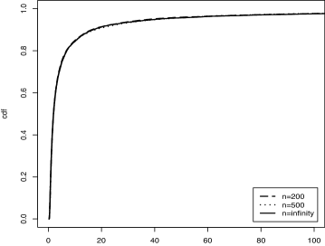
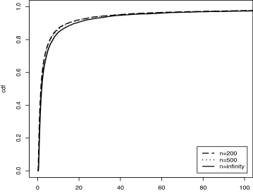
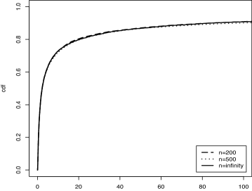
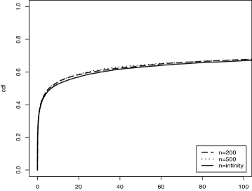
Figure 2. Empirical distributions of the re-scaled MLE at zero when sampling from the Beta distribution (left) and the Gamma distribution (right): from top to bottom we have $\alpha=0.2,0.5,0.8$.

3. Some Numerical Results

Figure 2 gives plots of the empirical distributions of $m=10000$ Monte Carlo samples from the distributions of $\widehat{f}_{n}(0)/(C_{2}n^{\alpha}/(1-\alpha))^{1/(1-\alpha)})$ when $n=200$ and $n=500$, together with the limiting distribution function obtained in (1.9). The true density $f_{0}$ on the right side in Figure 2 is

(3.20) $$f_{0}(x)=\int_{0}^{\infty}\frac{1}{y}1_{[0,y]}(x)\frac{y^{c-1}}{\Gamma(c)}\exp(-y)dy;$$

For $c\in(0,1)$, this family satisfies (G2) with $\alpha=1-c$ and $C_{2}=1/(\alpha\Gamma(1-\alpha))$. (Note that for $c=1$, $f_{0}(x)\sim\log(1/x)$ as $x\searrow 0$.)

The true density $f_{0}$ on the left side in Figure 2 is

(3.21) $$f_{0}(x)=\frac{1}{\mbox{Beta}(1-a,2)}x^{-a}(1-x)1_{(0,1]}(x);$$

For $a\in[0,1)$, this family satisfies (G2) with $\alpha=a$ and $C_{2}=1/\mbox{Beta}(1-\alpha,2)$.

Figure 3. Empirical distributions of the supremum measure: the cutoff values shown are $c=5$ (top left), $c=25$ (top right), $c=100$ (bottom left), $c=1000$ (bottom right).

Figure 3 shows simulations of the limiting distribution

(3.22) $$\sup_{0\leq t\leq c}\left|t^{1-\gamma}\widehat{h}(t)/\gamma-1\right|$$

for different values of $c$ and $\gamma$. Recall that if $\gamma=1$ the supremum occurs at $t=0$ regardless of the value of $c$, and the limiting distribution (3.22) has cumulative distribution function $1-1/(x+1).$ However, for $\gamma<1$, the distribution of (3.22) depends both on $\gamma$ and on $c$, although the dependence on $c$ is not visually prominent in Figure 3. Table 1 shows estimated values of

(3.23) $$P\left(\sup_{0\leq t\leq c}|t^{1-\gamma}\widehat{h}(t)/\gamma-1|=1\right)$$

for different $c$ and $\gamma<1$, which clearly depends on the cutoff value $c$ (upper bound on the standard deviation in each case is 0.016). Note that (3.22) is equal to one if the location of the supremum occurs at $t=0$ (with probability one).

Table 1. Simulation of (3.23) for different values of $\gamma$ and $c$.

	$c=0.5$	$c=5$	$c=25$	$c=100$	$c=1000$
$\gamma=0.25$	0.361	0.171	0.140	0.092	0.06
$\gamma=0.50$	0.422	0.249	0.190	0.162	0.148
$\gamma=0.75$	0.489	0.387	0.349	0.358	0.367

Cumulative distribution functions for the location of the supremum in (3.22) are shown in Figure 4, which clearly depend both on $\gamma$ and on $c$.

Figure 4. Empirical distributions of the location where the supremum occurs: from left to right we have $\gamma=0.25,0.50,0.75$. Recall that for $\gamma=1$, the (non-unique) location of the supremum is always zero by Corollary 1.2. The data were re-scaled to lie within the interval $[0,1]$.

4. Application to Mixtures

4.1. Behavior near zero

First, suppose that $X_{1},\ldots,X_{n}$ are i.i.d. with distribution function $F$ where,

$$\mbox{under}\ H_{0}:\ F=\Phi_{r},\qquad\mbox{the generalized normal distribution}$$

$$\mbox{under}\ H_{1}:\ F=(1-\epsilon)\Phi_{r}+\epsilon\Phi_{r}(\cdot-\mu),\ \ \epsilon\in(0,1),\ \ \mu>0,$$

where $\Phi_{r}(x)\equiv\int_{-\infty}^{x}\phi_{r}(y)dy$ with $\phi_{r}(y)\equiv\exp(-|y|^{r}/r)/C_{r}$ for $r>0$ gives the generalized normal (or Subbotin) distribution; here $C_{r}\equiv 2\Gamma(1/r)r^{(1/r)-1}$ is the normalizing constant. If we transform to $Y_{i}\equiv 1-\Phi_{r}(X_{i})\sim G$, then, for $0~{}\leq~{}y~{}\leq~{}1$,

$$\mbox{under}\ H_{0}:G(y)=y,\qquad\mbox{the Uniform}(0,1)\ \mbox{d.f.},$$

$$\mbox{under}\ H_{1}:G(y)=G_{\epsilon,\mu,r}(y)=(1-\epsilon)y+\epsilon(1-\Phi_{r}(\Phi_{r}^{-1}(1-y)-\mu)).$$

Let $g_{\epsilon,\mu,r}$ denote the density of $G_{\epsilon,\mu,r}$; thus

(4.24) $$\hskip 28.45274ptg_{\epsilon,\mu,r}(y) = 1-\epsilon+\epsilon\exp\left\{-\frac{1}{r}\left(|\Phi_{r}^{-1}(1-y)-\mu|^{r}-|\Phi_{r}^{-1}(1-y)|^{r}\right)\right\}.$$

It is easily seen that $g_{\epsilon,\mu,r}$ is monotone decreasing on $(0,1)$ and is unbounded at zero if $r>1$. Figure 5 shows plots of these densities for $\epsilon=.1$, $\mu=1$, and $r\in\{1.0,1.1,\ldots,2.0\}$. Note that $g_{\epsilon,\mu,1}$ is bounded at $0$: in fact $g_{\epsilon,\mu,1}(y)=1-\epsilon+\epsilon e^{\mu}$ for $0\leq y\leq 2^{-1}e^{-\mu}$.

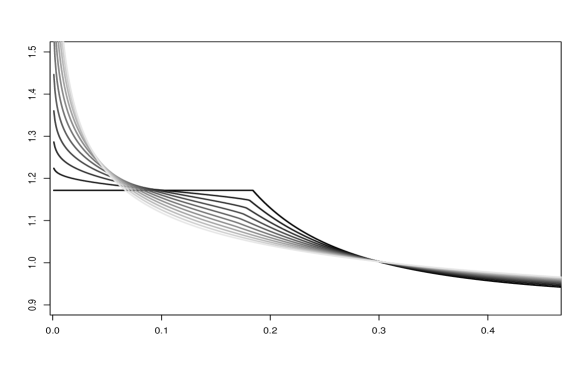
Figure 5. Generalized Gaussian (or Subbotin) mixture densities with $\epsilon=.1$, $\mu=1$, $r\in\{1.0,1.2,\ldots,2.0\}$ (black to light grey, respectively) as given by (4.24).

Proposition 4.1.

The distribution $F_{\mu,r}(y)\equiv 1-\Phi_{r}(\Phi_{r}^{-1}(1-y)-\mu)$ is regularly varying at $0$ with exponent $1$. That is, for any $c>0$,

$$\lim_{y\rightarrow 0+}\frac{F_{\mu,r}(cy)}{F_{\mu,r}(y)}=c,$$

i.e. (1.5) holds with $\gamma=1$.

Proof. Define $\kappa_{r}(y)=\Phi_{r}^{-1}(1-y).$ Our first goal will be to show that

(4.25) $$\lim_{y\rightarrow 0}\frac{\kappa_{r}(y)}{\tilde{\kappa}_{r}(y)}=1,$$

where (for $y$ small)

$$\tilde{\kappa}_{r}(y)=\left(-r\log\left({C_{r}\ y\ \left\{r\log\left(\frac{1}{C_{r}y}\right)\right\}^{(r-1)/r}}\right)\right)^{1/r}.$$

To prove (4.25), it is enough to show that

(4.26) $$\lim_{y\rightarrow 0}{\tilde{\kappa}_{r}(y)^{r-1}}(\kappa_{r}(y)-\tilde{\kappa}_{r}(y))=0.$$

This result follows from de Haan and Ferreira (2006, Theorem 1.1.2). Define

$$b_{n}=\tilde{\kappa}_{r}(1/n),\ \ \ a_{n}=1/b_{n}^{r-1},$$

and choose $F=\Phi_{r}$ in the statement of Theorem 1.1.2. Then, if we can show that

(4.27) $$n(1-\Phi_{r}(a_{n}x+b_{n}))\rightarrow\log G(x)\equiv e^{-x},\qquad x\in{\mathbb{R}},$$

it follows from de Haan and Ferreira (2006, Theorem 1.1.2 and Section 1.1.2) that for all $x\in{\mathbb{R}}$

$$\lim_{y\rightarrow 0}\frac{U(x/y)-b_{\lfloor 1/y\rfloor}}{a_{\lfloor 1/y\rfloor}}=G^{-1}(e^{-1/x})=\log(1/x),$$

where $U(t)=(1/(1-\Phi_{r}))^{-1}(t)=\Phi_{r}^{-1}(1-1/t).$ Choosing $x=1$ yields (4.26). Therefore, we need to prove (4.27).

To do this, we make use of the following, which is a generalization of Mills’ ratio to the generalized Gaussian family

(4.28) $$1-\Phi_{r}(z)\sim\frac{\phi_{r}(z)}{z^{r-1}}\qquad\mbox{as}\ \ z\rightarrow\infty.$$

The statement follows from l’Hôpital’s rule:

$$\lim_{z\rightarrow\infty}\frac{\int_{z}^{\infty}\phi_{r}(y)dy}{z^{1-r}\phi_{r}(z)} = \lim_{z\rightarrow\infty}\frac{-\phi_{r}(z)}{(1-r)z^{-r}\phi_{r}(z)+z^{1-r}\phi_{r}(z)(-z^{r-1})}$$

$$= \lim_{z\rightarrow\infty}\frac{1}{1-(1-r)z^{-r}}=1.$$

Now,

$$n(1-\Phi_{r}(a_{n}x+b_{n})) \sim n\frac{\phi_{r}(a_{n}x+b_{n})}{(a_{n}x+b_{n})^{r-1}}$$

$$= \frac{n}{C_{r}b_{n}^{r-1}}\frac{\exp\left(-\frac{b_{n}^{r}}{r}\left(1+\frac{a_{n}x}{b_{n}}\right)^{r}\right)}{(1+a_{n}x/b_{n})^{r-1}}$$

$$\sim \frac{n}{C_{r}b_{n}^{r-1}}\exp\left(-\frac{b_{n}^{r}}{r}\left(1+\frac{rx}{b_{n}^{r}}\right)\right)$$

$$= \exp\left(-\left(\frac{b_{n}^{r}}{r}+(r-1)\log b_{n}-\log n+\log C_{r}\right)\right)\exp(-x)$$

$$\rightarrow \exp(-0)\cdot\exp(-x)$$

by using the definition of $b_{n}$. We have thus shown that (4.25) holds.

Then, for $y\rightarrow 0$, by (4.28) and (4.25)

$$F_{\mu,r}(y) = 1-\Phi_{r}(\kappa_{r}(y)-\mu)\sim 1-\Phi_{r}(\tilde{\kappa}_{r}(y)-\mu)$$

$$\sim \frac{\phi_{r}(\tilde{\kappa}_{r}(y)-\mu)}{(\tilde{\kappa}_{r}(y)-\mu)^{r-1}}.$$

Plugging in the definition of $\phi_{r},$ we find that

$$F_{\mu,r}(y) \sim \frac{1/C_{r}}{(\tilde{\kappa}_{r}(y)-\mu)^{r-1}}\exp\left(-\frac{\tilde{\kappa}_{r}(y)^{r}}{r}\left|1-\frac{\mu}{\tilde{\kappa}_{r}(y)}\right|^{r}\right)$$

$$= \frac{1/C_{r}}{(\tilde{\kappa}_{r}(y)-\mu)^{r-1}}\exp\left\{\left(\log(C_{r}y)+\log(r\log(1/(C_{r}y)))\right)\left|1-\frac{\mu}{\tilde{\kappa}_{r}(y)}\right|^{r}\right)$$

$$= \frac{1/C_{r}}{(\tilde{\kappa}_{r}(y)-\mu)^{r-1}}\ (C_{r}y)^{\left|1-\frac{\mu}{\tilde{\kappa}_{r}(y)}\right|^{r}}\cdot\left\{r\log\frac{1}{C_{r}y}\right\}^{\frac{r-1}{r}\left|1-\frac{\mu}{\tilde{\kappa}_{r}(y)}\right|^{r}}.$$

Note that $\lim_{y\rightarrow 0}\tilde{\kappa}_{r}(cy)/\tilde{\kappa}_{r}(y)=1$. Therefore,

$$\frac{F_{\mu,r}(cy)}{F_{\mu,r}(y)} \sim c^{\left|1-\frac{\mu}{\tilde{\kappa}_{r}(cy)}\right|^{r}}\cdot(C_{r}y)^{{\left|1-\frac{\mu}{\tilde{\kappa}_{r}(cy)}\right|^{r}}-{\left|1-\frac{\mu}{\tilde{\kappa}_{r}(y)}\right|^{r}}}\cdot\left(\frac{\tilde{\kappa}_{r}(y)-\mu}{\tilde{\kappa}_{r}(cy)-\mu}\right)^{r-1}$$

$$\qquad\cdot\frac{\left\{r\log\frac{1}{C_{r}cy}\right\}^{\frac{r-1}{r}\left|1-\frac{\mu}{\tilde{\kappa}_{r}(cy)}\right|^{r}}}{\left\{r\log\frac{1}{C_{r}y}\right\}^{\frac{r-1}{r}\left|1-\frac{\mu}{\tilde{\kappa}_{r}(y)}\right|^{r}}}$$

$$\rightarrow c\cdot 1\cdot 1\cdot 1=c.$$

Thus (1.5) holds with $\gamma=1$. $\Box$

By the theory of regular variation (see e.g. Bingham et al. (1989, page 21)), this implies that $F_{\mu,r}(y)=y\ell(y)$ where $\ell$ is slowly varying at $0$. It then follows easily that (1.5) holds for $F_{0}=G_{\epsilon,\mu,r}$ with exponent $1$. Thus our theory of Section 1 applies with $a_{n}$ of Theorem 1.1 taken to be $a_{n}=G_{\epsilon,\mu,\gamma}(1/n)$; i.e.

$$\frac{1}{n}=G_{\epsilon,\mu,r}(a_{n})=(1-\epsilon)a_{n}+\epsilon F_{\mu,r}(a_{n})\ \dot{=}\ \epsilon F_{\mu,r}(a_{n})$$

where the last approximation is valid for $r>1$, but not for $r=1$. When $r=1$, the first equality can be solved explicitly, and we find:

(4.31) $$a_{n}=\left\{\begin{array}[]{l l}1-\Phi_{r}(\Phi_{r}^{-1}(1-(1/(n\epsilon)))+\mu),&\mbox{when}\ \ r>1\\ n^{-1}(1-\epsilon+\epsilon e^{\mu})^{-1},&\mbox{when}\ \ r=1.\end{array}\right.$$

We conclude that Theorem 1.1 holds for $a_{n}$ as in the last display where $\widehat{f}_{n}$ is the Grenander estimator of $g_{\epsilon,\mu,r}$ based on $Y_{1},\ldots,Y_{n}$.

Another interesting mixture family to consider is as follows: suppose that $\Phi_{1}$, $\Phi_{2}$ are two fixed distribution functions: then

$$\mbox{under}\ H_{0}:\ F=\Phi_{1},$$

$$\mbox{under}\ H_{1}:\ F=(1-\epsilon)\Phi_{1}+\epsilon\Phi_{2},\ \ \epsilon\in(0,1).$$

Using the transformation to $Y_{i}\equiv 1-\Phi_{1}(X_{i})\sim G$, then, for $0\leq y\leq 1$ we find that under $H_{1}$ the distribution of the $Y_{i}$’s is given by

$$G(y)=(1-\epsilon)y+\epsilon(1-\Phi_{2}(\Phi_{1}^{-1}(1-y))),$$

$$g(y)=(1-\epsilon)+\epsilon\frac{\phi_{2}(\Phi_{1}^{-1}(1-y))}{\phi_{1}(\Phi_{1}^{-1}(1-y))}.$$

For $\Phi_{2}$ given in terms of $\Phi_{1}$ by the (Lehmann alternative) distribution function $\Phi_{2}(y)=1-(1-\Phi_{1}(y))^{\gamma}$, this becomes

$$G(y)=(1-\epsilon)y+\epsilon y^{\gamma},$$

$$g(y)=(1-\epsilon)+\epsilon\gamma y^{\gamma-1}.$$

When $0<\gamma<1$ this family fits into the framework of our condition G2 with $\alpha=1-\gamma$ and $C_{2}=\epsilon\gamma$.

4.2. Estimation of the contaminating density

Suppose that $G_{\epsilon,F}(y)=(1-\epsilon)y+\epsilon F(y)$ where $F$ is a concave distribution on $[0,1]$ with monotone decreasing density $f$. Thus the density $g_{\epsilon,F}$ of $G_{\epsilon,F}$ is given by $g_{\epsilon,F}(y)=(1-\epsilon)+\epsilon f(y)$. Note that $g_{\epsilon,F}$ is also monotone decreasing, and $g_{\epsilon,F}(y)\geq 1-\epsilon+\epsilon f(1)=1-\epsilon=g_{\epsilon,F}(1)$ if $f(1)=0$. For $\epsilon>0$ we can write

$$f(y)=\frac{g_{\epsilon,F}(y)-(1-\epsilon)}{\epsilon}.$$

If $Y_{1},\ldots,Y_{n}$ are i.i.d. $g_{\epsilon,F}$ then we can estimate $g_{\epsilon,F}$ by the Grenander estimator $\widehat{g}_{n}$, and we can estimate $\epsilon$ by

$$\widehat{\epsilon}_{n}=1-\widehat{g}_{n}(1).$$

This results in the following estimator $\widehat{f}_{n}$ of the contaminating density $f$:

$$\widehat{f}_{n}(y)=\frac{\widehat{g}_{n}(y)-(1-\widehat{\epsilon}_{n})}{\widehat{\epsilon}_{n}}=\frac{\widehat{g}_{n}(y)-\widehat{g}_{n}(1)}{1-\widehat{g}_{n}(1)},$$

which is quite similar in spirit to a setting studied by Swanepoel (1999). Here, however, we propose using the shape constraint of monotonicity, and hence the Grenander estimator, to estimate both $\epsilon$ and $f$. We intend to study this estimator elsewhere.

Appendix A: Proofs for Section 1

Before proving Theorem 1.1, we need the following two lemmas. The first lemma shows that the functionals $\mathop{\rm{argmax}\mathstrut}\nolimits^{R}$ and $\mathop{\rm{argmax}\mathstrut}\nolimits^{L}$ are both $O_{p}(1)$, while the second shows these are equivalent almost surely for the limiting Poisson process. Together, these two lemmas will show that both functionals $\mathop{\rm{argmax}\mathstrut}\nolimits^{R}$ and $\mathop{\rm{argmax}\mathstrut}\nolimits^{L}$ are continuous. Below we assume that (1.5) holds and that $nF_{0}(a_{n})\sim 1$. Thus both (1.3) and (1.7) also hold.

Lemma 5.2.

(i)  When $\gamma=1$ and $x>1$, $\mbox{argmax}_{v}^{L,R}\{n{\mathbb{F}}_{n}(a_{n}v)-xv\}=O_{p}(1)$.
(ii)  When $\gamma\in(0,1)$ and $x>0$, $\mbox{argmax}_{v}^{L,R}\{n{\mathbb{F}}_{n}(a_{n}v)-xv\}=O_{p}(1)$.

Proof. It suffices to show that

$$\limsup_{n\rightarrow\infty}P(\sup_{v\geq K}\{n{\mathbb{F}}_{n}(a_{n}v)-xv\}\geq 0)\rightarrow 0,\ \ \mbox{as}\ \ K\rightarrow\infty$$

under the conditions specified. Let $h(x)=x(\log x-1)+1$ and recall the inequality

$$P(\mbox{Bin}(n,p)/(np)\geq t)\leq\exp(-nph(t))$$

for $t\geq 1$ where $\mbox{Bin}(n,p)$ denotes a Binomial$(n,p)$ random variable; see e.g. Shorack and Wellner (1986, inequality 10.3.2, page 415). It follows that

(5.32) $$P(\sup_{v\geq K}\{n{\mathbb{F}}_{n}(a_{n}v)-xv\}\geq 0)$$

$$= P(\cup_{j=K}^{\infty}\{n{\mathbb{F}}_{n}(a_{n}v)-xv\geq 0\ \ \mbox{for some}\ \ v\in[j,j+1)\})$$

$$\leq \sum_{j=K}^{\infty}P(n{\mathbb{F}}_{n}(a_{n}(j+1))-xj\geq 0)$$

$$= \sum_{j=K}^{\infty}P\left(\frac{n{\mathbb{F}}_{n}(a_{n}(j+1))}{nF_{0}(a_{n}(j+1))}\geq\frac{xj}{nF_{0}(a_{n}(j+1))}\right)$$

$$\leq \sum_{j=K}^{\infty}\exp\left(-nF_{0}(a_{n}(j+1))h\left(\frac{xj}{nF_{0}(a_{n}(j+1))}\right)\right)$$

Next, since $F_{0}$ is concave,

$$nF_{0}(a_{n}(j+1))\leq nF_{0}(a_{n}(K+1))\frac{j+1}{K+1}$$

for $j\geq K$ and $nF_{0}(a_{n}(K+1))\rightarrow(K+1)^{\gamma}$ and $n\rightarrow\infty$. Therefore, for all $j\geq K$ and sufficiently large $n$, we have

$$\frac{xj}{nF_{0}(a_{n}(j+1))}\geq\delta(K+1)^{1-\gamma}\frac{xj}{j+1}$$

for any fixed $\delta<1.$ We need to handle the two cases $\gamma=1$ and $\gamma<1$ separately. Note that if $\gamma<1$, then the above display shows that $K,n$ can be chosen sufficiently large so that $(xj)/nF_{0}(a_{n}(j+1))$ is uniformly large. On the other hand, if $\gamma=1$ and $x>1$ then we can pick $\delta,K,n$ large enough so that $(xj)/nF_{0}(a_{n}(j+1))$ is strictly greater than $1+\epsilon$ for some $\epsilon>0$, again uniformly in $j$.

Suppose first that $\gamma<1$. Then for $K,n$ large, since $h(x)\sim x\log x$ as $x\rightarrow\infty$, there exists a constant $0<C<1$ such that for all $j\geq K$

$$nF_{0}(a_{n}(j+1))h\left(\frac{xj}{nF_{0}(a_{n}(j+1))}\right) \geq C(xj)\log\left(\frac{xj}{j+1}\right)$$

$$\geq C_{x}(xj),$$

for some other constant $C_{x}>0$. This shows that the sum in (5.32) converges to zero as $K\rightarrow\infty,$ as required.

Suppose next that $\gamma=1$. Note that the function $h(x)>0$ for $x>1$. Therefore, combining our arguments above, we find that for all $j\geq K$

$$nF_{0}(a_{n}(j+1))h\left(\frac{xj}{nF_{0}(a_{n}(j+1))}\right) \geq \delta(j+1)h\left(\frac{xj}{nF_{0}(a_{n}(j+1))}\right)$$

$$\geq C_{x,\delta}(j+1),$$

again for some $C_{x,\delta}>0$. This again implies that the sum in (5.32) converges to zero as $K\rightarrow\infty,$ and completes the proof. $\Box$

Lemma 5.3.

Suppose that $\gamma\in(0,1]$. Then

$$V_{x}^{L}\equiv\mathop{\rm{argmax}\mathstrut}\nolimits_{v}^{L}\{{\mathbb{N}}(v^{\gamma})-xv\}=\mathop{\rm{argmax}\mathstrut}\nolimits_{v}^{R}\{{\mathbb{N}}(v^{\gamma})-xv\}\equiv V_{x}^{R}\qquad a.s.$$

Proof. Suppose that $V_{x}^{L}<V_{x}^{R}$. Then it follows that ${\mathbb{N}}((V_{x}^{L})^{\gamma})-xV_{x}^{L}={\mathbb{N}}((V_{x}^{R})^{\gamma})-xV_{x}^{R}$, or, equivalently

$${\mathbb{N}}((V_{x}^{R})^{\gamma})-{\mathbb{N}}((V_{x}^{L})^{\gamma})=x\{V_{x}^{R}-V_{x}^{L}\}.$$

Now $(V_{x}^{R})^{\gamma},\ (V_{x}^{L})^{\gamma}\in J({\mathbb{N}})\equiv\{t>0:\ {\mathbb{N}}(t)-{\mathbb{N}}(t-)\geq 1\}$, so the left side of the last display takes values in the set $\{1,2,\ldots\}$, while the right side takes values in $x\cdot\{r^{1/\gamma}-s^{1/\gamma}:\ r,s\in J({\mathbb{N}}),r>s\}$. But it is well-known that all the (joint) distributions of the points in $J({\mathbb{N}})$ are absolutely continuous with respect to Lebesgue measure, and hence the equality in the last display holds only for sets with probability $0$. $\Box$

Proof of Theorem 1.1: We first prove convergence of the one-dimensional distributions of $na_{n}\widehat{f}_{n}(a_{n}t)$. Fix $K>0$, and let $x>1_{\{\gamma=1\}}$ and $t\in(0,K]$. By the switching relation (2.12),

$$P(na_{n}\widehat{f}_{n}(a_{n}t)\leq x) = P(\widehat{s}_{n}^{L}(x/(na_{n}))\leq a_{n}t)$$

$$= P(\mbox{argmax}_{s}^{L}\{{\mathbb{F}}_{n}(s)-xs/(na_{n})\}\leq a_{n}t)$$

$$= P(\mbox{argmax}_{v}^{L}\{{\mathbb{F}}_{n}(va_{n})-x(v/n)\}\leq t)$$

$$= P(\mbox{argmax}_{v}^{L}\{n{\mathbb{F}}_{n}(va_{n})-xv\}\leq t)$$

$$\rightarrow P(\mbox{argmax}_{v}^{L}\{{\mathbb{N}}(v^{\gamma})-xv\}\leq t)$$

$$= P(\widehat{h}_{\gamma}(t)\leq x)$$

where the convergence follows from (1.7), and the argmax continuous mapping theorem for $D[0,\infty)$ applied to the processes $\{v\mapsto n{\mathbb{F}}_{n}(va_{n})-xv:\ v\geq 0\}$; see e.g. Ferger (2004, Theorem 3 and Corollary 1). Note that Lemma 5.2 yields the $O_{p}(1)$ hypothesis of Ferger’s Corollary 1, while Lemma 5.3 shows that equality holds in the limit conclusion.

Convergence of the finite-dimensional distributions of $\widehat{h}_{n}(t)\equiv na_{n}\widehat{f}_{n}(a_{n}t)$ follows in the same way by using the process convergence in (1.7) for finitely many values $(t_{1},x_{1}),\ldots,(t_{m},x_{m})$ where each $t_{j}\in{\mathbb{R}}^{+}$ and $x_{j}>1_{\{\gamma=1\}}$.

To verify tightness of $\widehat{h}_{n}$ in $D[0,\infty)$ we use Billingsley (1999, Theorem 16.8). Thus, it is sufficient to show that for any $K>0$, and any $\epsilon>0$

(5.33) $$\lim_{M\rightarrow\infty}\limsup_{n}P\left(\sup_{0\leq t\leq K}|\widehat{h}_{n}(t)|\geq M\right) = 0$$

(5.34) $$\lim_{\delta\rightarrow 0}\limsup_{n}P\left(w_{\delta,K}(\widehat{h}_{n})\geq\epsilon\right) = 0,$$

where $w_{\delta,K}(h)$ is the modulus of continuity in the Skorohod topology defined as

$$w_{\delta,K}(h) = \inf_{\{t_{i}\}_{r}}\max_{0<i\leq r}\sup\left\{|h(t)-h(s)|:s,t\in[t_{i-1},t_{i})\cap[0,K]\right\},$$

where $\{t_{i}\}_{r}$ is a partition of $[0,K]$ such that $0=t_{0}<t_{1}<\ldots<t_{r}=K$ and $t_{i}-t_{i-1}>\delta$. Suppose then that $h$ is a piecewise constant function with discontinuities occurring at the (ordered) points $\{\tau_{i}\}_{i\geq 0}$. Then if $\delta\leq\inf_{i}|\tau_{i}-\tau_{i-1}|$ we necessarily have that $w_{\delta,K}(h)=0.$

First, note that since $\widehat{h}_{n}$ is non-increasing,

$$\|\widehat{h}_{n}\|_{0}^{m}\equiv\sup_{0\leq t\leq m}|\widehat{h}_{n}(t)|=\widehat{h}_{n}(0),$$

and hence (5.33) follows from the finite-dimensional convergence proved above.

Next, fix $\epsilon>0$. Let $0=\tau_{n,0}<\tau_{n,1}<\cdots<\tau_{n,K_{n}}<K$ denote the (ordered) jump points of $\widehat{h}_{n}$, and let $0=T_{n,0}<T_{n,1}<\cdots<T_{n,J_{n}}<K$ denote the (again, ordered) jump points of $n{\mathbb{F}}_{n}(a_{n}t)$. Because $\{\tau_{n,1},\ldots,\tau_{n,K_{n}}\}\subset\{T_{n,1},\ldots,T_{n,J_{n}}\}$, it follows that $\inf\{\tau_{i,n}-\tau_{i-1,n}\}\geq\inf\{T_{i,n}-T_{i-1,n}\}$ and hence

$$P\left(w_{\delta,K}(\widehat{h}_{n})\geq\epsilon\right)\leq P\left(\inf_{i=1,\ldots,J_{n}}\{T_{i,n}-T_{i-1,n}\}<\delta\right).$$

Now, by (1.7) and continuity of the inverse map (see e.g. Whitt (2002, Theorem 13.6.3, page 446))

$$(T_{n,1},\ldots,T_{n,J_{n}},0,0,\ldots)\Rightarrow(T_{1}^{1/\gamma},\ldots,T_{J}^{1/\gamma},0,0,\ldots),$$

where $T_{1},\ldots,T_{J}$ denote the successive arrival times on $[0,K]$ of a standard Poisson process. Thus,

$$\lim_{\delta\rightarrow 0}P\left(\inf_{i=1,\ldots,J}\{T_{i}^{1/\gamma}-T_{i-1}^{1/\gamma}\}<\delta\right)=0.$$

and therefore (5.34) holds. This completes the proof of (i).

Now we prove (ii): Fix $0<c<\infty$. We first write

(5.35) $$\sup_{0<x\leq ca_{n}}\left|\frac{\widehat{f}_{n}(x)}{f_{0}(x)}-1\right| = \sup_{0<t\leq c}\left|\frac{na_{n}\widehat{f}_{n}(ta_{n})}{na_{n}f_{0}(ta_{n})}-1\right|.$$

Suppose we could show that the ratio process $na_{n}\widehat{f}_{n}(a_{n}t)/na_{n}f_{0}(a_{n}t)$ converges to the process $t^{1-\gamma}\widehat{h}_{\gamma}(t)/\gamma$ in $D[0,\infty)$. Then the conclusion follows by noting that the functional $h\mapsto\sup_{0<t\leq c}|h|$ is continuous in the Skorohod topology as long as $c$ is not a point of discontinuity of $h$ (Jacod and Shiryaev (2003, Proposition VI 2.4, page 339)). Since ${\mathbb{N}}(t^{\gamma})$ is stochastically continuous (i.e. $P({\mathbb{N}}(t^{\gamma})-{\mathbb{N}}(t^{\gamma}-)>0)=0$ for each fixed $t>0$), $t^{1-\gamma}\widehat{h}_{\gamma}(t)/\gamma$ is almost surely continuous at $c$.

It remains to prove convergence of the ratio. Fix $K>c$, and again we may assume that $K$ is a continuity point. Consider first the term in the denominator, $na_{n}f_{0}(a_{n}t)$: it follows from (1.4) that

$$g_{n}(t)\equiv(na_{n}f_{0}(a_{n}t))^{-1}\rightarrow\gamma^{-1}t^{1-\gamma}\equiv g(t)$$

where $g$ is monotone increasing and uniformly continuous on $[0,K]$. Thus $g_{n}\rightarrow g$ in $C[0,K]$. Since the term in the numerator satisfies $h_{n}(t)\equiv na_{n}\widehat{f}_{n}(a_{n}t)\Rightarrow\widehat{h}_{\gamma}(t)\equiv h(t)$ in $D[0,K]$, it follows that $g_{n}h_{n}\Rightarrow gh$ in $D[0,K]$, as required. Here, we have again used the continuity of the supremum. This completes the proof of (ii). $\Box$

Before proving Corollaries 1.2 - 1.4 we state the following lemma.

Lemma 5.4.

Suppose that $a_{n}=p(1/n)$ for some function with $p(0)=0$ satisfying $\lim_{x\rightarrow 0+}p^{\prime}(x)f_{0}(p(x))=1$. Then $nF_{0}(a_{n})\rightarrow 1$.

Proof: This follows easily from l’Hôpital’s rule, since

$$\lim_{n\rightarrow\infty}nF_{0}(a_{n})=\lim_{x\rightarrow 0+}\frac{F_{0}(p(x))}{x}=\lim_{x\rightarrow 0+}f_{0}(p(x))p^{\prime}(x).$$

$\Box$

Proof of Corollary 1.2: Under the assumption G0 we see that $F_{0}(x)\sim f_{0}(0+)x$ as $x\rightarrow 0$, so (1.5) holds with $\gamma=1$. The claim that $a_{n}=1/(nf_{0}(0+))$ satisfies $nF_{0}(a_{n})\rightarrow 1$ follows from Lemma 5.4 with $p(x)=x/f_{0}(0+)$. For (i) note that $\widehat{h}_{1}(0)=\widehat{h}_{1}(0+)=\sup_{t>0}({\mathbb{N}}(t)/t)$, and the indicated equality in distribution follows from Pyke (1959); see Proposition 1.5 and its proof. (ii) follows directly from (i) of Theorem 1.1. To prove (iii), note that from (ii) of Theorem 1.1 it suffices to show that

(5.36) $$\sup_{0<t\leq c}\left|\widehat{h}_{1}(t)-1\right|=\left|\widehat{h}_{1}(0+)-1\right|=\widehat{h}_{1}(0+)-1=Y_{1}-1$$

for each $c>0$ where $\widehat{h}_{1}(t)$ is the right derivative of the LCM of ${\mathbb{N}}(t)$. The equality in (5.36) holds if $\widehat{h}_{1}(c)>1$, since $\widehat{h}_{1}$ is decreasing by definition. By the switching relation (2.12), we have the equivalence

$$\{\widehat{h}_{1}(c)>1\}=\{\widehat{s}^{L}(1)>c\}.$$

The equality in (5.36) thus follows if $\widehat{s}^{L}(1)=\infty$. That is, if

$${\mathbb{N}}(t)-t<\sup_{y\geq 0}\{{\mathbb{N}}(y)-y\}\ \ \mbox{ for all finite }t.$$

Let $W=\sup_{y\geq 0}\{{\mathbb{N}}(y)-y\}$. Pyke (1959, pages 570-571) showed that $P(W\leq x)=0$ for $x\geq 0$; i.e. $P(W=\infty)=1$. $\Box$

Proof of Corollary 1.3: Under the assumption G1 we see that $F_{0}(x)\sim C_{1}x(\log(1/x))^{\beta}$ as $x\rightarrow 0$, so (1.5) holds with $\gamma=1$. The claim that $a_{n}=1/(C_{1}n(\log n)^{\beta})$ satisfies $nF_{0}(a_{n})\rightarrow 1$ follows from Lemma 5.4 with $p(x)=x/(C_{1}\log(1/x))^{\beta}$. For (i) note that $\widehat{h}_{1}(0)=\widehat{h}_{1}(0+)=\sup_{t>0}({\mathbb{N}}(t)/t)$ just as in the proof of Corollary 1.2. (ii) again follows directly from (i) of Theorem 1.1, and the proof of (iii) is just the same as in the proof of Corollary 1.2. $\Box$

Proof of Corollary 1.4: Under the assumption G2 we see that $F_{0}(x)\sim C_{2}x^{1-\alpha}/(1-\alpha)$ as $x\rightarrow 0$, so (1.5) holds with $\gamma=1-\alpha$. The claim that $a_{n}=\{(1-\alpha)/(nC_{2})\}^{1/(1-\alpha)}$ satisfies $nF_{0}(a_{n})\rightarrow 1$ follows from Lemma 5.4 with $p(x)=((1-\alpha)x/C_{2})^{1/(1-\alpha)}$. For (i) note that

$$\widehat{h}_{1-\alpha}(0)=\widehat{h}_{1-\alpha}(0+)=\sup_{t>0}({\mathbb{N}}(t^{1-\alpha})/t)=\sup_{s>0}({\mathbb{N}}(s)/s^{1/(1-\alpha)})$$

much as in the proof of Corollary 1.2. (ii) and (iii) follow directly from (i) and (ii) of Theorem 1.1. $\Box$

Proof of Proposition 1.5: The part of the proposition with $\gamma=1$ follows from Pyke (1959, pages 570-571); this is closely related to a classical result of Daniels (1945) for the empirical distribution function; see e.g. Shorack and Wellner (1986, Theorem 9.1.2, page 345).

The proof for the case $\gamma<1$ proceeds much along the lines of Mason (1983, pages 103–105). Fix $x>0$ and $\gamma<1$. We aim at establishing an expression for the distribution function of $Y_{\gamma}\equiv\sup_{s>0}({\mathbb{N}}(s)/s^{1/\gamma})$ at $x>0$. First, observe that

(5.37) $$P(Y_{\gamma}\leq x) = P\left(\sup_{s>0}\left\{\frac{{\mathbb{N}}(s)}{s^{1/\gamma}}\right\}\leq x\right)$$

$$= P({\mathbb{N}}(t)\leq U(t)\ \quad\text{for all $t>0$})$$

where the function $U(t)=xt^{1/\gamma}$. For $j\in{\mathbb{N}}$ let $t_{j}:=(j/x)^{\gamma}$, and note that $t_{1}<t_{2}<~{}\ldots$ and $U(t_{j})=j$.

Define sets $B$ and $C$ by

$$B\equiv[{\mathbb{N}}(t_{k})\neq k\,;\text{ for all $k\geq 1$}]\ \ \mbox{and}\ \ C\equiv[{\mathbb{N}}(s)>U(s)\,;\text{ for some $s>0$}].$$

Then $P(B\cap C)=0$ as a consequence of the following argument: Suppose that there exists some $t>0$ and $k\in{\mathbb{N}}$ such that $k={\mathbb{N}}(t)>U(t)$ and ${\mathbb{N}}(t_{i})\neq i$, for all $i\geq 1$. It then follows that $t_{k}>t$, for otherwise it follows that $k=U(t_{k})\leq U(t)$, as $U(\cdot)$ is increasing, which is a contradiction. Therefore, $t_{k}>t$ implies that ${\mathbb{N}}(t_{k})>{\mathbb{N}}(t)=k$, as ${\mathbb{N}}(\cdot)$ is non–decreasing while ${\mathbb{N}}(t_{k})=k$ is disallowed, by hypothesis. Hence, ${\mathbb{N}}(t_{i})>i$ holds true for all $i\geq k$, for otherwise there would exist some $j\geq k$ such that ${\mathbb{N}}(t_{j})=j$, since ${\mathbb{N}}(\cdot)$ is a counting process. Therefore, for each $i\geq k$ we have that ${\mathbb{N}}(s)\geq i+1$ holds for all $t_{i}\leq s\leq t_{i+1}$ and, consequently, that ${\mathbb{N}}(s)\geq U(s)$ holds for all $s\geq t_{k}$. This implies that $B\cap C\subseteq[\liminf_{s\to\infty}\{{\mathbb{N}}(s)/s^{1/\gamma}\}\geq x]$ and therefore $P(B\cap C)=0$, since the SLLN implies that ${\mathbb{N}}(s)/s^{1/\gamma}\rightarrow 0$ holds almost surely, for fixed $\gamma<1$. We thus conclude that $P(B\cap C)=0$.

We conclude that $P(C)=P(C\cap B^{c})$. Furthermore, since $U$ is a strictly increasing function, and since ${\mathbb{N}}$ has jumps at the points $\{t_{k}\}$ with probability zero, we also find that $P(C\cap B^{c})=P(B^{c})$. Finally, partition $B^{c}$ as $B^{c}=\cup_{k=1}^{\infty}A_{k}$ for the disjoint sets $A_{k}\equiv[{\mathbb{N}}(t_{k})=k,{\mathbb{N}}(t_{j})\neq j\text{ for all $1\leq j<k$}]$, $k\geq 1$. Combining all arguments above, we conclude that

$$P(Y_{\gamma}\leq x)=1-P(C)=1-\sum_{k=1}^{\infty}P(A_{k})$$

where $P(A_{1})=P({\mathbb{N}}(t_{1})=1)=p(t_{1};1)$, and, for $k\geq 2$, $P(A_{k})$ may be written as

$$P({\mathbb{N}}(t_{k})=k)-P(\{{\mathbb{N}}(t_{k})=k\}\cap\{{\mathbb{N}}(t_{i})\not=i,\,i<k\}^{c})$$

$$= P({\mathbb{N}}(t_{k})=k)-\sum_{j=1}^{k-1}P({\mathbb{N}}(t_{k})=k,\,{\mathbb{N}}(t_{j})=j,\,{\mathbb{N}}(t_{i})\not=i,\,i<j)$$

$$= P({\mathbb{N}}(t_{k})=k)-\sum_{j=1}^{k-1}P({\mathbb{N}}(t_{k})-{\mathbb{N}}(t_{j})=k-j)P({\mathbb{N}}(t_{j})=j,{\mathbb{N}}(t_{i})\not=i,\,i<j).$$

The result follows. $\Box$

Appendix B: Definitions from Convex Analysis

The epigraph (hypograph) of a function $f$ from a subset $S$ of ${\mathbb{R}}^{d}$ to $[-\infty,+\infty]$ is the subset $\mbox{epi}(f)$ ($\mbox{hypo}(f)$) of ${\mathbb{R}}^{d+1}$ defined by

$$\mbox{epi}(f) = \{(x,t):\,x\in S,\,t\in{\mathbb{R}},\,t\geq f(x)\},$$

$$\mbox{hypo}(f) = \{(x,t):\ x\in S,\,t\in{\mathbb{R}};\ t\leq f(x)\}.$$

The function $f$ is convex if $\mbox{epi}(f)$ is a convex set. The effective domain of a convex function $f$ on $S$ is

$$\mbox{dom}(f)=\{x\in{\mathbb{R}}^{d}:\,(x,t)\in\mbox{epi}(f)\ \mbox{for some }\ t\}=\{x\in{\mathbb{R}}^{d}:\ f(x)<\infty\}.$$

The $t-$sublevel set of a convex function $f$ is the set $C_{t}=\{x\in\mbox{dom}(f):\ f(x)\leq t\},$ and the $t-$superlevel set of a concave function $g$ is the set $S_{t}=\{x\in\mbox{dom}(g):\ g(x)\geq t\}.$ The sets $C_{t}$, $S_{t}$ are convex. The convex hull of a set $S\subset{\mathbb{R}}^{d}$, denoted by $\mbox{conv}(S)$, is the intersection of all the convex sets containing $S$.

A convex function $f$ is said to be proper if its epigraph is non-empty and contains no vertical lines; i.e. if $f(x)<+\infty$ for at least one $x$ and $f(x)>-\infty$ for every $x$. Similarly, a concave function $g$ is proper if the convex function $-g$ is proper. The closure of a concave function $g$, denoted by $\mbox{cl}(g)$, is the pointwise infimum of all affine functions $h\geq g$. If $g$ is proper, then

$$\mbox{cl}(g)(x)=\limsup_{y\rightarrow x}g(y).$$

For every proper convex function $f$ there exists closed proper convex function $\mathop{\mathrm{cl}\mathstrut}\nolimits(f)$ such that $\mbox{epi}(\mathop{\mathrm{cl}\mathstrut}\nolimits(f))\equiv\mathop{\mathrm{cl}\mathstrut}\nolimits(\mbox{epi}(f))$. The conjugate function $g^{*}$ of a concave function $g$ is defined by

$$g^{*}(y)=\inf\{\langle x,y\rangle-g(x):\ x\in{\mathbb{R}}^{d}\},$$

and the conjugate function $f^{*}$ of a convex function $f$ is defined by

$$f^{*}(y)=\sup\{\langle x,y\rangle-f(x):\ x\in{\mathbb{R}}^{d}\}.$$

If $g$ is concave, then $f=-g$ is convex and $f$ has conjugate $f^{*}(y)=-g^{*}(-y)$.

A complete non-decreasing curve is a subset of ${\mathbb{R}}^{2}$ of the form

$$\Gamma=\{(x,y):\ x\in{\mathbb{R}},\ y\in{\mathbb{R}},\ \varphi_{-}(x)\leq y\leq\varphi_{+}(x)\}$$

for some non-decreasing function $\varphi$ from ${\mathbb{R}}$ to $[-\infty,+\infty]$ which is not everywhere infinite. Here $\varphi_{+}$ and $\varphi_{-}$ denote the right and left continuous versions of $\varphi$ respectively. A vector $y\in{\mathbb{R}}^{d}$ is said to be a subgradient of a convex function $f$ at a point $x$ if

$$f(z)\geq f(x)+\langle y,z-z\rangle\qquad\mbox{for all}\ \ z\in{\mathbb{R}}^{d}.$$

The set of all subgradients of $f$ at $x$ is called the subdifferential of $f$ at $x$, and is denoted by $\partial f(x)$.

A face of a convex set $C$ is a convex subset $B$ of $C$ such that every closed line segment in $C$ with a relative interior point in $B$ has both endpoints in $B$. If $B$ is the set of points where a linear function $h$ achieves its maximum over $C$, then $B$ is a face of $C$. If the maximum is achieved on the relative interior of a line segment $L\subset C$, then $h$ must be constant on $L$ and $L\subset B$. A face $B$ of this type is called an exposed face.

Centre de Recherche en Mathématiques de la Décision
Université Paris-Dauphine, Paris, France E-mail: fadoua@ceremade.dauphine.fr Department of Mathematics and Statistics
York University, Toronto, Canada E-mail: hkj@mathstat.yorku.ca Department of Mechanical Engineering
Frederick University Cyprus, Nicosia, Cyprus E-mail: m.pavlides@frederick.ac.cy Department of Statistics
University of Washington, Seattle, USA E-mail: arseni@stat.washington.edu Department of Statistics
University of Washington, Seattle, USA E-mail: jaw@stat.washington.edu

References

- Anevski and Soulier (2009) Anevski, D. and Soulier, P. (2009). Monotone spectral density estimation. Tech. rep., University of Lund, Department of Mathematics.
- Beran (1994) Beran, J. (1994). Statistics for long-memory processes, vol. 61 of Monographs on Statistics and Applied Probability. Chapman and Hall, New York.
- Billingsley (1999) Billingsley, P. (1999). Convergence of Probability Measures. 2nd ed. John Wiley & Sons Inc., New York.
- Bingham et al. (1989) Bingham, N. H., Goldie, C. M. and Teugels, J. L. (1989). Regular Variation, vol. 27 of Encyclopedia of Mathematics and its Applications. Cambridge University Press, Cambridge.
- Boyd et al. (2004) Boyd, S. and Vandenberghe, L. (2004). Convex Optimization. Cambridge University Press, Cambridge.
- Cox (1984) Cox, D. R. (1984). Long-range dependence: A review. In Statistics: An Appraisal (H. A. David and H. T. David, eds.). Iowa State University.
- Daniels (1945) Daniels, H. E. (1945). The statistical theory of the strength of bundles of threads. I. Proc. Roy. Soc. London. Ser. A. 183 405–435.
- de Haan and Ferreira (2006) de Haan, L. and Ferreira, A. (2006). Extreme Value Theory. Springer Series in Operations Research and Financial Engineering, Springer, New York.
- Devroye (1986) Devroye, L. (1986). Nonuniform Random Variate Generation. Springer-Verlag, New York.
- Devroye (1987) Devroye, L. (1987). A Course in Density Estimation, vol. 14 of Progress in Probability and Statistics. Birkhäuser Boston Inc., Boston, MA.
- Donoho and Jin (2004) Donoho, D. and Jin, J. (2004). Higher criticism for detecting sparse heterogeneous mixtures. Ann. Statist. 32 962–994.
- Ferger (2004) Ferger, D. (2004). A continuous mapping theorem for the argmax-functional in the non-unique case. Statist. Neerlandica 58 83–96.
- Gnedenko (1943) Gnedenko, B. (1943). Sur la distribution limite du terme maximum d’une série aléatoire. Ann. of Math. (2) 44 423–453.
- Gneiting (2000) Gneiting, T. (2000). Power-law correlations, related models for long-range dependence and their simulation. J. Appl. Probab. 37 1104–1109.
- Grenander (1956a) Grenander, U. (1956a). On the theory of mortality measurement. I. Skand. Aktuarietidskr. 39 70–96.
- Grenander (1956b) Grenander, U. (1956b). On the theory of mortality measurement. II. Skand. Aktuarietidskr. 39 125–153 (1957).
- Groeneboom (1985) Groeneboom, P. (1985). Estimating a monotone density. In Proceedings of the Berkeley conference in honor of Jerzy Neyman and Jack Kiefer, Vol. II (Berkeley, Calif., 1983). Wadsworth Statist./Probab. Ser., Wadsworth, Belmont, CA.
- Jacod and Shiryaev (2003) Jacod, J. and Shiryaev, A. N. (2003). Limit Theorems for Stochastic Processes, vol. 288 of Grundlehren der Mathematischen Wissenschaften [Fundamental Principles of Mathematical Sciences]. 2nd ed. Springer-Verlag, Berlin.
- Kulikov and Lopuhaä (2005) Kulikov, V. N. and Lopuhaä, H. P. (2005). Asymptotic normality of the -error of the Grenander estimator. Ann. Statist. 33 2228–2255.
- Kulikov and Lopuhaä (2006) Kulikov, V. N. and Lopuhaä, H. P. (2006). The behavior of the NPMLE of a decreasing density near the boundaries of the support. Ann. Statist. 34 742–768.
- Ma (2002) Ma, C. (2002). Correlation models with long-range dependence. J. Appl. Probab. 39 370–382.
- Martin and Walker (1997) Martin, R. J. and Walker, A. M. (1997). A power-law model and other models for long-range dependence. J. Appl. Probab. 34 657–670.
- Mason (1983) Mason, D. M. (1983). The asymptotic distribution of weighted empirical distribution functions. Stochastic Process. Appl. 15 99–109.
- Miller (1976) Miller, D. R. (1976). Order statistics, Poisson processes and repairable systems. J. Appl. Probability 13 519–529.
- Pyke (1959) Pyke, R. (1959). The supremum and infimum of the Poisson process. Ann. Math. Statist. 30 568–576.
- Rockafellar (1970) Rockafellar, R. T. (1970). Convex Analysis. Princeton Mathematical Series, No. 28, Princeton University Press, Princeton, N.J.
- Rockafellar and Wets (1998) Rockafellar, R. T. and Wets, R. J.-B. (1998). Variational Analysis, vol. 317 of Grundlehren der Mathematischen Wissenschaften [Fundamental Principles of Mathematical Sciences]. Springer-Verlag, Berlin.
- Shorack and Wellner (1986) Shorack, G. R. and Wellner, J. A. (1986). Empirical Processes with Applications to Statistics. Wiley Series in Probability and Mathematical Statistics: Probability and Mathematical Statistics, John Wiley & Sons Inc., New York.
- Swanepoel (1999) Swanepoel, J. W. H. (1999). The limiting behavior of a modified maximal symmetric -spacing with applications. Ann. Statist. 27 24–35.
- van de Geer (1993) van de Geer, S. (1993). Hellinger-consistency of certain nonparametric maximum likelihood estimators. Ann. Statist. 21 14–44.
- van der Vaart and van der Laan (2006) van der Vaart, A. and van der Laan, M. J. (2006). Estimating a survival distribution with current status data and high-dimensional covariates. Int. J. Biostat. 2 Art. 9, 42.