Restoration of the chiral limit
in Pauli–Villars-regulated light-front QED

Abstract

The dressed-electron eigenstate of Feynman-gauge QED is computed in light-front quantization with a Fock-space truncation to include at most the one-photon/one-electron sector. The theory is regulated by the inclusion of three massive Pauli–Villars (PV) particles, one PV electron, and two PV photons. In particular, the chiral limit is investigated, and the correct limit is found to require two PV photons, not just one as previously thought. The renormalization and covariance of the electron current are also analyzed. We find that the plus component is well behaved and use its spin-flip matrix element to compute the electron’s anomalous moment. The dependence of the moment on the regulator masses is shown to be slowly varying when the second PV photon is used to guarantee the correct chiral limit.

I Introduction

Over the past several years, a method of Pauli–Villars (PV) regularization PauliVillars has been developed for nonperturbative analysis of quantum field theories bhm1 ; bhm2 ; YukawaDLCQ ; ExactSolns ; YukawaOneBoson ; OnePhotonQED ; YukawaTwoBoson . It is based on the introduction of massive, negatively normed fields directly to the Lagrangian and the derivation of a light-front quantized Hamiltonian Dirac ; DLCQreview . The Hamiltonian is then used to construct an eigenvalue problem for the mass and Fock-state wave functions of bound states. The use of light-front quantization allows a meaningful Fock-state expansion with well-defined wave functions.

Bound-state problems in quantum field theories are notoriously difficult. Their nonperturbative nature complicates the regularization and renormalization. Of the various methods that have been attempted, such as lattice gauge theory lattice , Schwinger–Dyson equations SDE , and light-front quantization DLCQreview , only the light-front approach can provide well-defined wave functions.

To regulate the nonperturbative light-front problem, the regulators that work in perturbation theory and provide equivalence with Feynman perturbation theory are assumed to be sufficient. Careful studies of perturbative equivalence have been made by Paston et al Paston . To renormalize, the bare parameters of the Lagrangian are fixed via physical conditions, such as setting certain bound-state masses equal to measured values. This is distinct from the sector-dependent approach SectorDependent to renormalization, where the bare parameters are assigned different values in each Fock sector.

The purpose in studying QED with such a technique is to test methods in a gauge theory, the goal being to develop a method that works for bound states of QCD. There is no expectation that nonperturbative light-front results for QED will be at all competitive with high-order perturbative calculations Kinoshita . The numerical errors in solving the bound-state eigenvalue problem are currently of order 1%. For the calculation reported here, the Fock-space truncation is severe enough to make calculations tractable analytically, but not enough physics is included to expect close agreement with experiment. The main point of the calculation is instead that the behavior of the anomalous moment is now a slowly varying function of the regulator masses.

Specifically, we reconsider the dressed-electron state in Feynman-gauge QED truncated at the one-photon/one-electron Fock state. An earlier analysis OnePhotonQED was sufficient in a particular limit of Pauli–Villars masses. There, one PV electron and one PV photon were added to the Lagrangian to regulate the theory. The resulting bound-state problem was solved analytically, and the anomalous moment was calculated in the limit that the PV electron mass is taken to infinity.

When the PV electron mass is not infinite, however, the analysis breaks down, due to a violation of chiral symmetry in the massless electron limit. This violation was not recognized in the earlier work on this particular PV regularization OnePhotonQED but is quite consistent with what has been found in different PV regularizations of QED and Yukawa theory ChiralSymYukawa . We restore this symmetry by adding a second PV photon, with its coupling strength and mass related by a simple condition. We also verify that the electron one-loop self-energy is consistent with the Feynman result at the same order and show that the vertex and wave function renormalization constants, $Z_{1}$ and $Z_{2}$, are equal. However, the equality of $Z_{1}$ and $Z_{2}$ is effective only for the plus component of the current; our truncation destroys the covariance of the current, and only the plus component can be used.

With the second PV photon included, we are able to do a calculation of the electron’s anomalous moment at finite PV electron mass. The moment is computed from the spin-flip matrix element of the (unrenormalized) plus component of the current BrodskyDrell . We show that without the second PV photon, the anomalous moment has a strong dependence on the PV masses, and we identify the mechanism whereby restoration of the correct chiral limit removes the strong mass dependence.

The alternative, sector-dependent renormalization scheme SectorDependent has been employed in studies of light-front QED by Hiller and Brodsky hb and more recently by Karmanov et al. Karmanov:2006zf ; Bernard . Unfortunately, the most recent form of the sector-dependent approach Karmanov:2006zf leads to difficulties with the interpretation of the wave functions. The amplitude for the bare-electron state is of the form $\sqrt{1-\alpha J}$, where $J$ is a positive integral that is infinite when the regulators are removed. The probability of the one-photon/one-electron sector is $\alpha J$, and thus the norm is 1. For our case, the bare amplitude is $1/\sqrt{1+\alpha J}$ and the probability of the higher sector is $\alpha J/(1+\alpha J)$, again with a norm of 1. However, only in our case are there well-defined probabilities between zero and 1 for each Fock sector and for any value of $J$. What is more, if one calculates something directly from the wave functions of Karmanov et al., infinities are encountered before taking the regulator masses to infinity. For example, the expectation value of the number of photons in the dressed-electron state is infinite for finite PV masses, even in the one-photon truncation. An analogous calculation in QCD, such as a quark distribution function, would also yield infinity. In their method, useful information can be extracted from the wave functions only by embedding the eigenstate in a larger process and using an external probe combined with a separate renormalization of this external coupling, a process not so different from the effort required in lattice QCD, where wave functions are also not well defined.

Our calculations are done in terms of light-cone coordinates Dirac , which are defined by

$$x^{\pm}\equiv x^{0}\pm x^{3},\;\;\vec{x}_{\perp}\equiv(x^{1},x^{2}).$$ (1)

The covariant four-vector is written $x^{\mu}=(x^{+},x^{-},\vec{x}_{\perp})$. This corresponds to a spacetime metric of

$$g^{\mu\nu}=\left(\begin{array}[]{llll}0&2&0&0\\ 2&0&0&0\\ 0&0&-1&0\\ 0&0&0&-1\end{array}\right).$$ (2)

Dot products are then given by

$$x\cdot y=g_{\mu\nu}x^{\mu}y^{\nu}=\frac{1}{2}(x^{+}y^{-}+x^{-}y^{+})-\vec{x}_{\perp}\cdot\vec{y}_{\perp}.$$ (3)

For light-cone three-vectors we use the underscore notation

$$\underline{x}\equiv(x^{-},\vec{x}_{\perp}).$$ (4)

For momentum, the conjugate to $x^{-}$ is $p^{+}$, and, therefore, we use

$$\underline{p}\equiv(p^{+},\vec{p}_{\perp})$$ (5)

as the light-cone three-momentum. The dot product of momentum and position three-vectors is

$$\underline{p}\cdot\underline{x}\equiv\frac{1}{2}p^{+}x^{-}-\vec{p}_{\perp}\cdot\vec{x}_{\perp}.$$ (6)

The derivatives are

$$\partial_{+}\equiv\frac{\partial}{\partial x^{+}}\thinspace,\qquad\partial_{-}\equiv\frac{\partial}{\partial x^{-}}\thinspace,\qquad\partial_{i}\equiv\frac{\partial}{\partial x^{i}}.$$ (7)

The time variable is taken to be $x^{+}$, and time evolution of a system is then determined by ${\cal P}^{-}$, the operator associated with the momentum component conjugate to $x^{+}$. Stationary states are obtained as eigenstates of ${\cal P}^{-}$. As has been customary, we express the eigenvalue problem in terms of a light-cone Hamiltonian PauliBrodsky ; DLCQreview $H_{\rm LC}={\cal P}^{+}{\cal P}^{-}$ as

$$H_{\rm LC}|P\rangle=(M^{2}+P_{\perp}^{2})|P\rangle,\;\;\underline{\cal P}|P\rangle=\underline{P}|P\rangle,$$ (8)

where $M$ is the mass of the state, and ${\cal P}^{+}$ and $\vec{\cal P}_{\perp}$ are light-cone momentum operators. Without loss of generality, we will limit the total transverse momentum $\vec{P}_{\perp}$ to zero.

The structure of the remainder of the paper is as follows. In Sec. II we summarize the Feynman-gauge formulation of light-front QED, including two PV photons and one PV electron as regulators, and construct the Hamiltonian that defines the bound-state problem. We then give in Sec. III an update of the known analytic solution of the one-photon truncation OnePhotonQED to include the additional PV photon. The analysis of the electron self-energy, in particular the chiral limit, and of the renormalization of the current are discussed in Sec. IV. These developments are applied to the calculation of the anomalous moment in Sec. V, followed by a brief summary in Sec. VI. Appendices contain a discussion of the gauge condition and a proof of a useful identity for terms in the self-energy.

II Light-Front QED in Feynman Gauge

The Feynman-gauge QED Lagrangian, regulated by two PV photons and one PV electron, is

$${\cal L} = \sum_{i=0}^{2}(-1)^{i}\left[-\frac{1}{4}F_{i}^{\mu\nu}F_{i,\mu\nu}+\frac{1}{2}\mu_{i}^{2}A_{i}^{\mu}A_{i\mu}-\frac{1}{2}\left(\partial^{\mu}A_{i\mu}\right)^{2}\right]$$

$$+\sum_{i=0}^{1}(-1)^{i}\bar{\psi_{i}}(i\gamma^{\mu}\partial_{\mu}-m_{i})\psi_{i}-e\bar{\psi}\gamma^{\mu}\psi A_{\mu},$$

where

$$A_{\mu}=\sum_{i=0}^{2}\sqrt{\xi_{i}}A_{i\mu},\;\;\psi=\sum_{i=0}^{1}\psi_{i},\;\;F_{i\mu\nu}=\partial_{\mu}A_{i\nu}-\partial_{\nu}A_{i\mu}.$$ (10)

The subscript $i=0$ denotes a physical field and $i=1$ or 2 a PV field. Fields with odd index $i$ are chosen to be negatively normed. The mass of the physical photon, $\mu_{0}$, is set to zero.

The constants $\xi_{i}$ are introduced to adjust the couplings $\sqrt{\xi_{i}}e$ of the different photon flavors, in order to arrange the cancellations that are at the heart of PV regularization. The $\xi_{i}$ must satisfy constraints. One is simply that $\xi_{0}=1$, so that $e$ is the coupling of the physical electron to the physical photon. Another is to guarantee that summing over photon flavors, in an internal line of a Feynman graph, cancels the leading divergence associated with integration over the momentum of that line. Since the $i$th flavor has norm $(-1)^{i}$ and couples to a charge $\sqrt{\xi_{i}}e$ at each end, the constraint is

$$\sum_{i=0}^{2}(-1)^{i}\xi_{i}=0.$$ (11)

This also guarantees that $A^{\mu}$ in (10) is a zero-norm field. A third constraint will be imposed in Sec. IV, to obtain the correct chiral limit.

The dynamical fields are

$$\psi_{i+} = \frac{1}{\sqrt{16\pi^{3}}}\sum_{s}\int d\underline{k}\chi_{s}\left[b_{is}(\underline{k})e^{-i\underline{k}\cdot\underline{x}}+d_{i,-s}^{\dagger}(\underline{k})e^{i\underline{k}\cdot\underline{x}}\right]\,,$$ (12)

$$A_{i\mu} = \frac{1}{\sqrt{16\pi^{3}}}\int\frac{d\underline{k}}{\sqrt{k^{+}}}\left[a_{i\mu}(\underline{k})e^{-i\underline{k}\cdot\underline{x}}+a_{i\mu}^{\dagger}(\underline{k})e^{i\underline{k}\cdot\underline{x}}\right]\,,$$ (13)

with LepageBrodsky $\chi_{s}$ an eigenspinor of $\Lambda_{+}\equiv\gamma^{0}\gamma^{+}/2$. The creation and annihilation operators satisfy (anti)commutation relations

$$\{b_{is}(\underline{k}),b_{i^{\prime}s^{\prime}}^{\dagger}(\underline{k}^{\prime}\} = (-1)^{i}\delta_{ii^{\prime}}\delta_{ss^{\prime}}\delta(\underline{k}-\underline{k}^{\prime}),$$ (14)

$$\{d_{is}(\underline{k}),d_{i^{\prime}s^{\prime}}^{\dagger}(\underline{k}^{\prime}\} = (-1)^{i}\delta_{ii^{\prime}}\delta_{ss^{\prime}}\delta(\underline{k}-\underline{k}^{\prime}),$$ (15)

$${[}a_{i\mu}(\underline{k}),a_{i^{\prime}\nu}^{\dagger}(\underline{k}^{\prime}] = (-1)^{i}\delta_{ii^{\prime}}\epsilon^{\mu}\delta_{\mu\nu}\delta(\underline{k}-\underline{k}^{\prime}).$$ (16)

Here $\epsilon^{\mu}=(-1,1,1,1)$ is the metric signature for the photon field components in Gupta–Bleuler quantization GuptaBleuler ; GaugeCondition . For the zero-norm photon field $A_{\mu}$, we have $a_{\mu}=\sum_{i}\sqrt{\xi_{i}}a_{i\mu}$ and the commutator

$${[}a_{\mu}(\underline{k}),a_{\nu}^{\dagger}(\underline{k}^{\prime})]=\left[\sum_{i}(-1)^{i}\xi_{i}\right]\epsilon^{\mu}\delta_{\mu\nu}\delta(\underline{k}-\underline{k}^{\prime})=0.$$ (17)

The implementation of the gauge condition $\partial^{\mu}A_{i\mu}=0$ is discussed in Appendix A.

An important consequence of the regularization method is that one is not limited to light-cone gauge. The coupling of the two zero-norm fields $A^{\mu}$ and $\psi$ as the interaction term reduces the fermionic constraint equation to a solvable equation without forcing the gauge field $A_{-}=A^{+}$ to zero. The nondynamical components of the fermion fields satisfy the constraints ($i=0,1$)

$$i(-1)^{i}\partial_{-}\psi_{i-}+eA_{-}\sum_{j}\psi_{j-} = (i\gamma^{0}\gamma^{\perp})\left[(-1)^{i}\partial_{\perp}\psi_{i+}-ieA_{\perp}\sum_{j}\psi_{j+}\right]$$ (18)

$$-(-1)^{i}m_{i}\gamma^{0}\psi_{i+}.$$

It would appear that a nontrivial inversion of the covariant derivative is needed to solve these constraints, except when light-cone gauge ($A^{+}=0$) is used. However, if we subtract (18) for $i=1$ from (18) for $i=0$, the terms containing the gauge field cancel, and the constraint reduces to

$$i\partial_{-}(\psi_{0-}+\psi_{1-})=(i\gamma^{0}\gamma^{\perp})\partial_{\perp}(\psi_{0+}+\psi_{1+})-\gamma^{0}(m_{0}\psi_{0+}+m_{1}\psi_{1+}).$$ (19)

Thus, the nondynamical part of the null combination $\psi_{0}+\psi_{1}$ that couples to $A^{+}$ satisfies the same constraint as does the free fermion field. This constraint is then solved explicitly, and the nondynamical fermion fields are eliminated from the Lagrangian. The full Fermi field can then be written as

$$\psi_{i}=\frac{1}{\sqrt{16\pi^{3}}}\sum_{s}\int\frac{d\underline{k}}{\sqrt{k^{+}}}\left[b_{is}(\underline{k})e^{-i\underline{k}\cdot\underline{x}}u_{is}(\underline{k})+d_{i,-s}^{\dagger}(\underline{k})e^{i\underline{k}\cdot\underline{x}}v_{is}(\underline{k})\right],$$ (20)

and the light-cone Hamiltonian ${\cal P}^{-}$ can be constructed directly from the above Lagrangian.

Another important consequence of the regularization is the absence of instantaneous fermion contributions. The contributions from the instantaneous physical electron and the instantaneous PV electron cancel, because they are of opposite sign and are independent of the fermion mass.

The regularization scheme does have the disadvantage of breaking gauge invariance, through the presence of “flavor” changing currents where a physical fermion can be transformed to a PV fermion or vice versa. However, the breaking effects disappear in the limit of large PV fermion mass OnePhotonQED , because the physical fermion cannot make a transition to a state with infinite mass.

Without antifermion terms, the Hamiltonian is

$${\cal P}^{-}=\sum_{i,s}\int d\underline{p}\frac{m_{i}^{2}+p_{\perp}^{2}}{p^{+}}(-1)^{i}b_{i,s}^{\dagger}(\underline{p})b_{i,s}(\underline{p})$$

$$+\sum_{l,\mu}\int d\underline{k}\frac{\mu_{l}^{2}+k_{\perp}^{2}}{k^{+}}(-1)^{l}\epsilon^{\mu}a_{l\mu}^{\dagger}(\underline{k})a_{l\mu}(\underline{k})$$

$$+\sum_{i,j,l,s,\mu}\int d\underline{p}d\underline{q}\left\{b_{i,s}^{\dagger}(\underline{p})\left[b_{j,s}(\underline{q})V^{\mu}_{ij,2s}(\underline{p},\underline{q})\right.\right.$$

$$\left.\left.\rule{36.135pt}{0.0pt}+b_{j,-s}(\underline{q})U^{\mu}_{ij,-2s}(\underline{p},\underline{q})\right]\sqrt{\xi_{l}}a_{l\mu}^{\dagger}(\underline{q}-\underline{p})+H.c.\right\}.$$

This is a straightforward generalization of the Hamiltonian given in OnePhotonQED , to include the second PV photon and the $\xi$ factors. The vertex functions are the same, but are repeated here for convenience:

$$V^{0}_{ij\pm}(\underline{p},\underline{q}) = \frac{e}{\sqrt{16\pi^{3}}}\frac{\vec{p}_{\perp}\cdot\vec{q}_{\perp}\pm i\vec{p}_{\perp}\times\vec{q}_{\perp}+m_{i}m_{j}+p^{+}q^{+}}{p^{+}q^{+}\sqrt{q^{+}-p^{+}}},$$ (22)

$$V^{3}_{ij\pm}(\underline{p},\underline{q}) = \frac{-e}{\sqrt{16\pi^{3}}}\frac{\vec{p}_{\perp}\cdot\vec{q}_{\perp}\pm i\vec{p}_{\perp}\times\vec{q}_{\perp}+m_{i}m_{j}-p^{+}q^{+}}{p^{+}q^{+}\sqrt{q^{+}-p^{+}}},$$

$$V^{1}_{ij\pm}(\underline{p},\underline{q}) = \frac{e}{\sqrt{16\pi^{3}}}\frac{p^{+}(q^{1}\pm iq^{2})+q^{+}(p^{1}\mp ip^{2})}{p^{+}q^{+}\sqrt{q^{+}-p^{+}}},$$

$$V^{2}_{ij\pm}(\underline{p},\underline{q}) = \frac{e}{\sqrt{16\pi^{3}}}\frac{p^{+}(q^{2}\mp iq^{1})+q^{+}(p^{2}\pm ip^{1})}{p^{+}q^{+}\sqrt{q^{+}-p^{+}}},$$

$$U^{0}_{ij\pm}(\underline{p},\underline{q}) = \frac{\mp e}{\sqrt{16\pi^{3}}}\frac{m_{j}(p^{1}\pm ip^{2})-m_{i}(q^{1}\pm iq^{2})}{p^{+}q^{+}\sqrt{q^{+}-p^{+}}},$$

$$U^{3}_{ij\pm}(\underline{p},\underline{q}) = \frac{\pm e}{\sqrt{16\pi^{3}}}\frac{m_{j}(p^{1}\pm ip^{2})-m_{i}(q^{1}\pm iq^{2})}{p^{+}q^{+}\sqrt{q^{+}-p^{+}}},$$

$$U^{1}_{ij\pm}(\underline{p},\underline{q}) = \frac{\pm e}{\sqrt{16\pi^{3}}}\frac{m_{i}q^{+}-m_{j}p^{+}}{p^{+}q^{+}\sqrt{q^{+}-p^{+}}},$$

$$U^{2}_{ij\pm}(\underline{p},\underline{q}) = \frac{ie}{\sqrt{16\pi^{3}}}\frac{m_{i}q^{+}-m_{j}p^{+}}{p^{+}q^{+}\sqrt{q^{+}-p^{+}}}.$$

III One-Photon Truncation

The dressed-electron problem in QED has been solved analytically for a one-photon/one-electron truncation OnePhotonQED in the limit of an infinite PV electron mass. For calculations with higher-order truncation, even for a two-photon truncation, this infinite-mass limit cannot be taken explicitly. Therefore, the one-photon truncation must be studied for finite PV electron masses before proceeding to higher-order truncations. The eigenvalue problem is still analytically soluble; however, there are additional issues to be addressed in the renormalization, which we discuss in Sec. IV.

III.1 Electron Eigenstate

It is convenient to work in a Fock basis where ${\cal P}^{+}$ and $\vec{\cal P}_{\perp}$ are diagonal. We expand the eigenfunction for the dressed-electron state with total $J_{z}=\pm\frac{1}{2}$ in such a Fock basis as

$$|\psi^{\pm}(\underline{P})\rangle=\sum_{i}z_{i}b_{i\pm}^{\dagger}(\underline{P})|0\rangle+\sum_{ijs\mu}\int d\underline{k}C_{ijs}^{\mu\pm}(\underline{k})b_{is}^{\dagger}(\underline{P}-\underline{k})a_{j\mu}^{\dagger}(\underline{k})|0\rangle,$$ (23)

where we keep only the one-electron and one-photon/one-electron Fock sectors and have chosen the frame where the total transverse momentum is zero. The amplitudes $z_{i}$ and wave functions $C_{ijs}^{\mu\pm}$ that define this state must satisfy the coupled system of equations that results from the field-theoretic mass-squared eigenvalue problem (8) and satisfy the normalization condition

$$\langle\psi^{\sigma^{\prime}}(\underline{P}^{\prime})|\psi^{\sigma}(\underline{P})\rangle=\delta(\underline{P}^{\prime}-\underline{P})\delta_{\sigma^{\prime}\sigma}.$$ (24)

Careful interpretation of the solution is required to obtain physically meaningful answers. In particular, there needs to be a physical state with positive norm. We apply the same approach as was used in Yukawa theory YukawaOneBoson . A projection onto the physical subspace is accomplished by expressing Fock states in terms of positively normed creation operators $a_{0\mu}^{\dagger}$, $a_{2\mu}^{\dagger}$, and $b_{0s}^{\dagger}$ and the null combinations $a_{\mu}^{\dagger}=\sum_{i}\sqrt{\xi_{i}}a_{i\mu}^{\dagger}$ and $b_{s}^{\dagger}=b_{0s}^{\dagger}+b_{1s}^{\dagger}$. The $b_{s}^{\dagger}$ particles are annihilated by the generalized electromagnetic current $\bar{\psi}\gamma^{\mu}\psi$; thus, $b_{s}^{\dagger}$ creates unphysical contributions to be dropped, and, by analogy, we also drop contributions created by $a_{\mu}^{\dagger}$.

The projected dressed-fermion state is

$$|\psi_{\rm phys}^{\pm}(\underline{P})\rangle = \sum_{i}(-1)^{i}z_{i}b_{0\pm}^{\dagger}(\underline{P})|0\rangle$$

$$+\sum_{s\mu}\int d\underline{k}\sum_{i=0}^{1}\sum_{j=0,2}\sqrt{\xi_{j}}\sum_{k=j/2}^{j/2+1}\frac{(-1)^{i+k}}{\sqrt{\xi_{k}}}C_{iks}^{\mu\pm}(\underline{k})b_{0s}^{\dagger}(\underline{P}-\underline{k})a_{j\mu}^{\dagger}(\underline{k})|0\rangle.$$

This projection is to be used to compute the anomalous moment. We do not make the gauge projection $a_{j\mu}^{\dagger}\rightarrow\tilde{a}_{j\mu}^{\dagger}$ defined in (69), because gauge invariance has been broken by both the truncation and the flavor-changing currents. The remaining negative norm of $a_{j0}^{\dagger}$ does not cause difficulties for our calculations; in particular, the solution has positive norm.

III.2 Integral Equations

The amplitudes satisfy coupled equations that come from the basic eigenvalue equation $H_{\rm LC}|\psi\rangle=M^{2}|\psi\rangle$. These equations are, with $y=k^{+}/P^{+}$,

$$[M^{2}-m_{i}^{2}]z_{i} = \int P^{+}dyd^{2}k_{\perp}\sum_{j,l,\mu}\sqrt{\xi_{l}}(-1)^{j+l}\epsilon^{\mu}P^{+}\left[V_{ji+}^{\mu*}(\underline{P}-\underline{k},\underline{P})C^{\mu+}_{jl+}(\underline{k})\right.$$

$$\rule{144.54pt}{0.0pt}\left.+U_{ji+}^{\mu*}(\underline{P}-\underline{k},\underline{P})C^{\mu+}_{jl-}(\underline{k})\right],$$

and

$$\left[M^{2}-\frac{m_{i}^{2}+k_{\perp}^{2}}{(1-y)}-\frac{\mu_{l}^{2}+k_{\perp}^{2}}{y}\right]C^{\mu\pm}_{il\pm}(\underline{k}) = \sqrt{\xi_{l}}\sum_{j}(-1)^{j}z_{j}P^{+}V_{ij\pm}^{\mu}(\underline{P}-\underline{k},\underline{P}),$$ (27)

$$\left[M^{2}-\frac{m_{i}^{2}+k_{\perp}^{2}}{(1-y)}-\frac{\mu_{l}^{2}+k_{\perp}^{2}}{y}\right]C^{\mu\pm}_{il\mp}(\underline{k}) = \sqrt{\xi_{l}}\sum_{j}(-1)^{j}z_{j}P^{+}U_{ij\pm}^{\mu}(\underline{P}-\underline{k},\underline{P}).$$ (28)

The wave functions $C_{ils}^{\mu\pm}$ are obtained directly OnePhotonQED

$$C^{\mu\pm}_{il\pm}(\underline{k}) = \sqrt{\xi_{l}}\frac{\sum_{j}(-1)^{j}z_{j}P^{+}V_{ij\pm}^{\mu}(\underline{P}-\underline{k},\underline{P})}{M^{2}-\frac{m_{i}^{2}+k_{\perp}^{2}}{1-y}-\frac{\mu_{l}^{2}+k_{\perp}^{2}}{y}},$$ (29)

$$C^{\mu\pm}_{il\mp}(\underline{k}) = \sqrt{\xi_{l}}\frac{\sum_{j}(-1)^{j}z_{j}P^{+}U_{ij\pm}^{\mu}(\underline{P}-\underline{k},\underline{P})}{M^{2}-\frac{m_{i}^{2}+k_{\perp}^{2}}{1-y}-\frac{\mu_{l}^{2}+k_{\perp}^{2}}{y}}.$$ (30)

These can be eliminated from the first of the coupled equations to yield

$$(M^{2}-m_{i}^{2})z_{i} = \int dy\;d^{2}k_{\perp}\sum_{\mu,i^{\prime},j,l}(-1)^{i^{\prime}+j+l}\xi_{l}z_{i^{\prime}}(P^{+})^{3}\epsilon^{\mu}$$

$$\times\frac{V^{\mu*}_{ji+}(\underline{P}-\underline{k},\underline{P})V^{\mu}_{ji^{\prime}+}(\underline{P}-\underline{k},\underline{P})+U^{\mu*}_{ji+}(\underline{P}-\underline{k},\underline{P})U^{\mu}_{ji^{\prime}+}(\underline{P}-\underline{k},\underline{P})}{M^{2}-\frac{m_{j}^{2}+k_{\perp}^{2}}{1-y}-\frac{\mu_{l}^{2}+k_{\perp}^{2}}{y}},$$

which, on use of the definitions (22) of the vertex functions, can be written more usefully as

$$(M^{2}-m_{i}^{2})z_{i}=2e^{2}\sum_{i^{\prime}}(-1)^{i^{\prime}}z_{i^{\prime}}\left[\bar{J}+m_{i}m_{i^{\prime}}\bar{I}_{0}-2(m_{i}+m_{i^{\prime}})\bar{I}_{1}\right],$$ (32)

with

$$\bar{I}_{n}(M^{2}) = \int\frac{dydk_{\perp}^{2}}{16\pi^{2}}\sum_{jl}\frac{(-1)^{j+l}\xi_{l}}{M^{2}-\frac{m_{j}^{2}+k_{\perp}^{2}}{1-y}-\frac{\mu_{l}^{2}+k_{\perp}^{2}}{y}}\frac{m_{j}^{n}}{y(1-y)^{n}}\,,$$ (33)

$$\bar{J}(M^{2}) = \int\frac{dydk_{\perp}^{2}}{16\pi^{2}}\sum_{jl}\frac{(-1)^{j+l}\xi_{l}}{M^{2}-\frac{m_{j}^{2}+k_{\perp}^{2}}{1-y}-\frac{\mu_{l}^{2}+k_{\perp}^{2}}{y}}\frac{m_{j}^{2}+k_{\perp}^{2}}{y(1-y)^{2}}.$$ (34)

The form of (32) matches that of the equivalent eigenvalue problem in Yukawa theory YukawaOneBoson , with the replacements $g^{2}\rightarrow 2e^{2}$, $\mu_{0}I_{1}\rightarrow-2\bar{I}_{1}$, and $\mu_{0}^{2}J\rightarrow\bar{J}$.

The integrals $\bar{I}_{0}$ and $\bar{J}$ satisfy an identity, $\bar{J}=M^{2}\bar{I}_{0}$. This was stated in OnePhotonQED without a proof being given. A new, simple proof can be found in Appendix B of this paper. With use of this identity, the eigenvalue problem reduces to the simpler form

$$(M^{2}-m_{i}^{2})z_{i}=2e^{2}\sum_{i^{\prime}}(-1)^{i^{\prime}}z_{i^{\prime}}\left[(M^{2}+m_{i}m_{i^{\prime}})\bar{I}_{0}-2(m_{i}+m_{i^{\prime}})\bar{I}_{1}\right].$$ (35)

III.3 Solution of the Eigenvalue Problem

The solution to the eigenvalue problem is OnePhotonQED

$$\alpha_{\pm}=\frac{(M\pm m_{0})(M\pm m_{1})}{8\pi(m_{1}-m_{0})(2\bar{I}_{1}\pm M\bar{I}_{0})},\;\;z_{1}=\frac{M\pm m_{0}}{M\pm m_{1}}z_{0},$$ (36)

with $z_{0}$ determined by normalization. The simplicity of this result is due in part to the algebraic simplification of (32) that comes from the identity $\bar{J}=M^{2}\bar{I}_{0}$.

The value of $m_{0}$ is determined by requiring $\alpha_{\pm}$ to be equal to the physical value of $\alpha$. For small values of the PV masses there may be no such solution; however, for reasonable values we do find at least one solution for each branch.

The plot in Fig. 1 shows $\alpha_{\pm}/\alpha$ as functions of $m_{0}$.

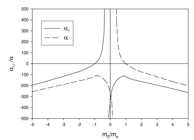
Figure 1: The two solutions of the one-photon eigenvalue problem, for PV masses $m_{1}=1000m_{e}$, $\mu_{1}=10m_{e}$, and $\mu_{2}=\infty$. The horizontal line shows where $\alpha_{\pm}=\alpha$. The $\alpha_{-}$ branch corresponds to the physical choice, but with $m_{0}$ less than $m_{e}$.

The $\alpha_{-}$ branch is the physical choice, because the no-interaction limit ($\alpha_{-}=0$) corresponds to the bare mass $m_{0}$ becoming equal to the physical electron mass, $M=m_{e}$.

If the PV electron has a sufficiently large mass, the value of $m_{0}$ that yields $\alpha_{-}=\alpha$ is less than $m_{e}$. In this case, the integrals $\bar{I}_{n}$ and $\bar{J}$ contain poles for $j=l=0$ and are defined by a principal-value prescription OnePhotonQED . The presence of the poles can then admit an additional delta-function term to the two-body wave function:

$$C_{00s}^{\mu\sigma}(\underline{k})\rightarrow C_{00s}^{\mu\sigma}(\underline{k})+c_{s}^{\mu\sigma}\delta(\underline{k}-\underline{k}_{0}),$$ (37)

where $\underline{k}_{0}$ is such that $M^{2}=\frac{m_{0}^{2}+k_{0\perp}^{2}}{1-y_{0}}+\frac{\mu_{0}^{2}+k_{0\perp}^{2}}{y_{0}}$. This remains a solution to (27), but there will be additional terms in (32) proportional to $c_{s}^{\mu\sigma}$. We do not explore this possibility, because we have found that when we include self-energy corrections from a two-photon truncation, the poles in these wave functions disappear.

III.4 Normalization

The normalization of the wave functions is determined by the condition in Eq. (24). In the case of the present truncation, this reduces to

$$1=|\sum_{i}(-1)^{i}z_{i}|^{2}+\sum_{s\mu}\int d\underline{k}\epsilon^{\mu}\sum_{j=0,2}\xi_{j}\left|\sum_{i=0}^{1}\sum_{k=j/2}^{j/2+1}\frac{(-1)^{i+k}}{\sqrt{\xi_{k}}}C_{iks}^{\mu+}(\underline{k})\right|^{2}.$$ (38)

For the given wave functions, after some tedious calculations, this becomes

$$\frac{1}{z_{0}^{2}} = (1-\zeta_{1})^{2}$$

$$+\frac{\alpha}{2\pi}\int ydydk_{\perp}^{2}\sum_{l,l^{\prime}}(-1)^{l+l^{\prime}}\zeta_{l}\zeta_{l^{\prime}}\sum_{i^{\prime}i}(-1)^{i^{\prime}+i}\sum_{j=0,2}\xi_{j}\sum_{k^{\prime}=j/2}^{j/2+1}\sum_{k=j/2}^{j/2+1}(-1)^{k^{\prime}+k}$$

$$\times\frac{m_{i^{\prime}}m_{i}-(m_{i}+m_{i^{\prime}})(m_{l}+m_{l^{\prime}})(1-y)+m_{l}m_{l^{\prime}}(1-y)^{2}+k_{\perp}^{2}}{[ym_{i^{\prime}}^{2}+(1-y)\mu_{k^{\prime}}^{2}+k_{\perp}^{2}-m_{e}^{2}y(1-y)][ym_{i}^{2}+(1-y)\mu_{k}^{2}+k_{\perp}^{2}-m_{e}^{2}y(1-y)]},$$

where $\zeta_{l}=z_{l}/z_{0}$.

For terms with $i=k=0$ or $i^{\prime}=k^{\prime}=0$, there are simple poles defined by a principal-value prescription. For the terms where all four of these indices are zero, there is a double pole, defined by the prescription OnePhotonQED

$$\int dx\frac{f(x)}{(x-a)^{2}}\equiv\lim_{\eta\rightarrow 0}\frac{1}{2\eta}\left[\mathcal{P}\int dx\frac{f(x)}{x-a-\eta}-\mathcal{P}\int dx\frac{f(x)}{x-a+\eta}\right].$$ (40)

One could instead compute the norm by taking the zero-momentum limit of the Dirac form factor, $F_{1}$; however, this would correspond to a more complicated point splitting. Our prescription splits only with respect to the magnitude of the momentum, rather than the magnitude and angle.

IV Regularization and Renormalization

To evaluate the usefulness of the chosen regularization, we consider three aspects. One is to compare the result for the one-loop electron self-energy with the standard result from covariant Feynman theory; we do this indirectly, by first comparing with the infinite-momentum-frame result of Brodsky, Roskies, and Suaya BRS , which they show to be consistent with Feynman theory. The second is to check the massless chiral limit, where we find a specific constraint on the PV photon masses and couplings. The third is to consider the renormalization of the external coupling to the charge. We exclude fermion-antifermion states, and, therefore, there is no vacuum polarization. Thus, if the vertex and wave function renormalizations cancel, there will be no renormalization of the external coupling. This is what we find, but only for the plus component of the current.

In our formulation, the perturbative one-loop electron self-energy can be read from Eq. (32) for $i=0$, with $z_{1}=0$, $M^{2}=m_{0}^{2}+\delta m^{2}$ on the left, and $M^{2}=m_{0}^{2}$ on the right. This yields

$$\delta m^{2}=2e^{2}\left[\bar{J}(m_{0}^{2})+m_{0}^{2}\bar{I}_{0}(m_{0}^{2})-4m_{0}\bar{I}_{1}(m_{0}^{2})\right].$$ (41)

When $\delta m=\delta m^{2}/2m_{0}$ is written explicitly in terms of $\alpha=e^{2}/4\pi$ and the integrals (33) and (34), we have

$$\delta m=\frac{\alpha}{4\pi}\sum_{jl}(-1)^{j+l}\frac{\xi_{l}}{m_{0}}\int\frac{dy}{y}\frac{d^{2}k_{\perp}}{\pi}\frac{m_{0}^{2}-\frac{4m_{0}m_{j}}{1-y}+\frac{m_{j}^{2}+k_{\perp}^{2}}{(1-y)^{2}}}{m_{0}^{2}-\frac{m_{0}^{2}+k_{\perp}^{2}}{1-y}-\frac{\mu_{l}^{2}+k_{\perp}^{2}}{y}}.$$ (42)

To compare with BRS , where the self-energy is regulated with only one PV photon, we restrict the sum over $l$ to two terms, $l=0$ and $l=1$. In this case, the $j=0$ term matches the form of $\delta m_{a}$ in Eq. (3.40) of BRS , which we quote here

$$\delta m_{a}=\frac{e^{2}}{16\pi^{2}m_{0}}\int d^{2}k_{\perp}\int\frac{dx}{1-x}\left[\frac{m_{0}^{2}(2-2x-x^{2})-k_{\perp}^{2}}{\lambda^{2}(1-x)+k_{\perp}^{2}+m_{0}^{2}x^{2}}-\frac{m_{0}^{2}(2-2x-x^{2})-k_{\perp}^{2}}{\Lambda^{2}(1-x)+k_{\perp}^{2}+m_{0}^{2}x^{2}}\right].$$ (43)

The $j=0$ term of (42) takes this form after setting $y=1-x$, $\mu_{0}=\lambda$, and $\mu_{1}=\Lambda$ and making some algebraic rearrangements. Also, the $j=1$ term reduces to $\delta m_{b}$ in Eq. (3.41) of BRS in the limit $m_{1}\rightarrow\infty$. In general, it is in this limit that the instantaneous fermion contributions return to the theory, and the source of $\delta m_{b}$ is just this type of graph. Here we do not take this limit, and the $j=1$ term remains as written and yields a different form for $\delta m_{b}$. However, if Brodsky et al. had used our regularization, they would also obtain this different form. Thus, our regularization produces a one-loop self-energy correction which is consistent with BRS when the same regularization is used, namely one PV electron and two PV photons, since the subtractions of contributions from the PV particles have exactly the same forms. This, in turn, is consistent with the Feynman result.

Although consistent with the standard result when regulated in the same way, the one-loop self-energy in this regularization, whether by covariant methods, by the infinite-momentum frame approach, or by light-cone quantization, does not automatically have the correct massless limit of zero, and chiral symmetry is broken. Consider the mass shift $\delta m$ in terms of the integrals defined in (33) and (34). From (42) we have

$$\delta m=16\pi^{2}\frac{\alpha}{2\pi}\left[m_{0}\bar{I}_{0}(m_{0}^{2})-2\bar{I}_{1}(m_{0}^{2})\right].$$ (44)

In the chiral limit, $m_{0}\rightarrow 0$, we obtain

$$\delta m=-32\pi^{2}\frac{\alpha}{2\pi}\bar{I}_{1}(0),$$ (45)

with

$$\bar{I}_{1}(0)=\frac{m_{1}}{16\pi^{2}}\sum_{l}(-1)^{l}\xi_{l}\int dyd^{2}k_{\perp}\frac{1}{k_{\perp}^{2}+m_{1}^{2}y+\mu_{l}^{2}(1-y)}.$$ (46)

The integrals in $\bar{I}_{1}(0)$ can be easily done, to find

$$\delta m=-\frac{\alpha}{\pi}m_{1}\sum_{l}(-1)^{l}\xi_{l}\frac{\mu_{l}^{2}/m_{1}^{2}}{1-\mu_{l}^{2}/m_{1}^{2}}\ln(\mu_{l}^{2}/m_{1}^{2}).$$ (47)

Clearly, this is zero only if $m_{1}$ is infinite or the $\xi_{l}$ and masses $\mu_{l}$ satisfy the constraint

$$\sum_{l}(-1)^{l}\xi_{l}\frac{\mu_{l}^{2}/m_{1}^{2}}{1-\mu_{l}^{2}/m_{1}^{2}}\ln(\mu_{l}^{2}/m_{1}^{2})=0.$$ (48)

This cannot be satisfied without the introduction of a second PV photon.

When the PV electron mass is sufficiently large, the chiral-limit constraint can be approximated by

$$\sum_{l}(-1)^{l}\xi_{l}\mu_{l}^{2}\ln(\mu_{l}/m_{1})=0.$$ (49)

The solution to the set of constraints, Eq. (11) and (49) along with $\xi_{0}=1$ and $\mu_{0}=0$, is then

$$\xi_{1}=1+\xi_{2}\;\;\mbox{and}\;\;\xi_{2}=\frac{\mu_{1}^{2}\ln(\mu_{1}/m_{1})}{\mu_{2}^{2}\ln(\mu_{2}/m_{1})-\mu_{1}^{2}\ln(\mu_{1}/m_{1})}.$$ (50)

Without loss of generality, we require $\mu_{2}>\mu_{1}$, so that $\xi_{2}$ is positive.

In covariant perturbation theory, it is a consequence of the Ward identity that, order by order, the wave function renormalization constant $Z_{2}$ is equal to the vertex renormalization $Z_{1}$. As discussed in BRS , this equality holds true more generally for nonperturbative bound-state calculations. However, a Fock-space truncation can have the effect of destroying covariance of the electromagnetic current, so that some components of the current require renormalization despite the absence of vacuum polarization. In the particular case here, only couplings to the plus component are not renormalized. The lack of fermion-antifermion vertices destroys covariance.

To see that $Z_{1}=Z_{2}$ holds for the plus component, define a bare state $|\psi_{\rm bare}\rangle$ of the electron as a Fock-state expansion in which the one-electron state has amplitude 1. It is then related to the physical electron state by

$$|\psi_{\rm phys}\rangle=\sqrt{Z_{2}}|\psi_{\rm bare}\rangle.$$ (51)

The normalization of the physical state $\langle\psi_{\rm phys}(p^{\prime})|\psi_{\rm phys}(p)\rangle=\delta(\underline{p}^{\prime}-\underline{p})$ implies

$$\langle\psi_{\rm bare}(p^{\prime})|\psi_{\rm bare}(p)\rangle=Z_{2}^{-1}\delta(\underline{p}^{\prime}-\underline{p}).$$ (52)

Matrix elements of the current $J^{\mu}$ define $Z_{1}$ by

$$\langle\psi_{\rm bare}|J^{\mu}(0)|\psi_{\rm bare}\rangle=Z_{1}^{-1}\bar{u}(p)\gamma^{\mu}u(p).$$ (53)

For the plus component, this matrix element can also be calculated as BrodskyDrell

$$\langle\psi_{\rm bare}(p^{\prime})|J^{+}(0)|\psi_{\rm bare}(p)\rangle=2p^{+}F_{1{\rm bare}}(-(p^{\prime}-p)^{2}).$$ (54)

Because LepageBrodsky $\bar{u}(p)\gamma^{+}u(p)=2p^{+}$ and $F_{1{\rm bare}}(0)=Z_{2}^{-1}$, we find that $\langle\psi_{\rm bare}|J^{+}(0)|\psi_{\rm bare}\rangle$ is equal to both $2p^{+}Z_{2}^{-1}$ and $2p^{+}Z_{1}^{-1}$, and therefore we have $Z_{1}=Z_{2}$.

The calculation of the anomalous moment, discussed in the next section, can then proceed. It is based on matrix elements of the plus component and thus does not require additional renormalization.

V Anomalous Magnetic Moment

We start from the Brodsky–Drell formula for the anomalous moment derived in BrodskyDrell from the spin-flip matrix element of the electromagnetic current. In the one-photon truncation their formula reduces to

$$a_{e} = m_{e}\sum_{s\mu}\int d\underline{k}\epsilon^{\mu}\sum_{j=0,2}\xi_{j}\left(\sum_{i^{\prime}=0}^{1}\sum_{k^{\prime}=j/2}^{j/2+1}\frac{(-1)^{i^{\prime}+k^{\prime}}}{\sqrt{\xi_{k^{\prime}}}}C_{i^{\prime}k^{\prime}s}^{\mu+}(\underline{k})\right)^{*}$$

$$\times y\left(\frac{\partial}{\partial k_{x}}+i\frac{\partial}{\partial k_{y}}\right)\left(\sum_{i=0}^{1}\sum_{k=j/2}^{j/2+1}\frac{(-1)^{i+k}}{\sqrt{\xi_{k}}}C_{iks}^{\mu-}(\underline{k})\right).$$

The presence of the derivative of the wave function (see Eqs. (29) and (30)) implies that we may face a triple pole; however, these terms cancel, and the expression for the anomalous moment simplifies to

$$a_{e} = \frac{\alpha}{\pi}m_{e}\int y^{2}(1-y)dydk_{\perp}^{2}\sum_{l,l^{\prime}}(-1)^{l+l^{\prime}}z_{l}z_{l^{\prime}}m_{l}\sum_{j=0,2}\xi_{j}$$

$$\times\left(\sum_{i=0}^{1}\sum_{k=j/2}^{j/2+1}\frac{(-1)^{i+k}}{ym_{i}^{2}+(1-y)\mu_{k}^{2}+k_{\perp}^{2}-m_{e}^{2}y(1-y)}\right)^{2}.$$

The double pole is handled in the same way as for the normalization integrals, discussed in Sec. III.4. The integrals can be done analytically.

In the limit where the PV electron mass $m_{1}$ is infinite, the bare-electron amplitude ratio $z_{1}/z_{0}$ is zero but the limit of the product $m_{1}z_{1}/z_{0}$ is $m_{0}-m_{e}$. Thus, the limit of the expression for the anomalous moment is

$$a_{e}=\frac{\alpha}{\pi}m_{e}^{2}z_{0}^{2}\int y^{2}(1-y)dydk_{\perp}^{2}\sum_{j=0,2}\xi_{j}\left(\sum_{k=j/2}^{j/2+1}\frac{(-1)^{k}}{ym_{0}^{2}+(1-y)\mu_{k}^{2}+k_{\perp}^{2}-m_{e}^{2}y(1-y)}\right)^{2}.$$ (57)

This differs slightly from the expression given in Eq. (70) of OnePhotonQED , where only one PV photon was included, the projection onto physical states was not taken, and $m_{1}z_{1}$ was assumed to be zero; however, the difference in values is negligible when $\mu_{1}$ and $\mu_{2}$ are sufficiently large.

If the second PV photon is not included, the results for the anomalous moment have a very strong dependence on the PV masses $\mu_{1}$ and $m_{1}$, as shown in Fig. 2.

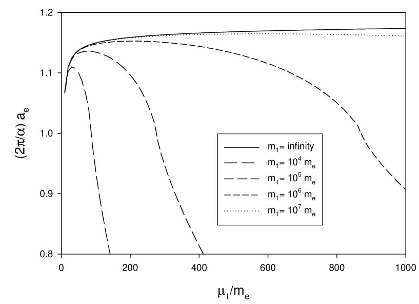
Figure 2: The anomalous moment of the electron in units of the Schwinger term (${\alpha/2\pi}$) plotted versus the PV photon mass, $\mu_{1}$, for a few values of the PV electron mass, $m_{1}$. The second PV photon is absent, and the chiral symmetry of the massless limit is broken by the remaining regularization.

A slowly varying behavior with respect to the PV photon mass $\mu_{1}$ is obtained only if the PV electron mass $m_{1}$ is (nearly) infinite.

The strong variation with $\mu_{1}$ when $m_{1}$ is finite is a consequence of broken chiral symmetry. This can be seen as follows. The anomalous moment is very sensitive to the masses of the constituents hb , and the mass $m_{0}$ of the electron constituent is determined by the eigenvalue solution (36), which contains the integral $\bar{I}_{1}$. Relative to the integral’s value $\bar{I}_{1\infty}$ at infinite $m_{1}$, we have

$$\bar{I}_{1}=\bar{I}_{1\infty}+\int\frac{dydk_{\perp}^{2}}{16\pi^{2}}\sum_{j}\frac{(-1)^{j}\xi_{j}m_{1}}{k_{\perp}^{2}+ym_{1}^{2}+(1-y)\mu_{j}^{2}-m_{e}^{2}y(1-y)}.$$ (58)

When $m_{e}$ is neglected compared to $m_{1}$, the second term becomes the chiral limit of $\bar{I}_{1}$, and this introduces a correction to the bare-electron mass of the form $\frac{\mu_{1}^{2}\ln(\mu_{1}/m_{1})}{8\pi^{2}m_{e}m_{1}(1-\mu^{2}/m_{1}^{2})}$. This correction is removed when the second PV photon is included, because the chiral limit of $\bar{I}_{1}$ is then zero, but when the correction is not removed, it injects a very strong dependence on $\mu_{1}$ and $m_{1}$ into the behavior of the bare mass $m_{0}$ and thus into the behavior of the anomalous moment.

From Fig. 2, we see that, without the second PV photon, the PV electron mass needs to be on the order of $10^{7}\,m_{e}$ before results for the one-photon truncation approach the infinite-mass limit. Thus, we estimate that the PV electron mass must be at least this large for a calculation with a two-photon Fock-space truncation, if only one PV photon is included. Unfortunately, such large mass values make numerical calculations difficult, because of contributions to integrals at momentum fractions of order $(m_{e}/m_{1})^{2}\simeq 10^{-14}$, which are then subject to large round-off errors. Therefore, a practical two-photon calculation will require the second PV photon.

We now repeat the calculation of the anomalous moment in the one-photon truncation with the second PV photon included. The result is given in Fig. 3 for PV masses related by $\mu_{2}=\sqrt{2}\mu_{1}$.

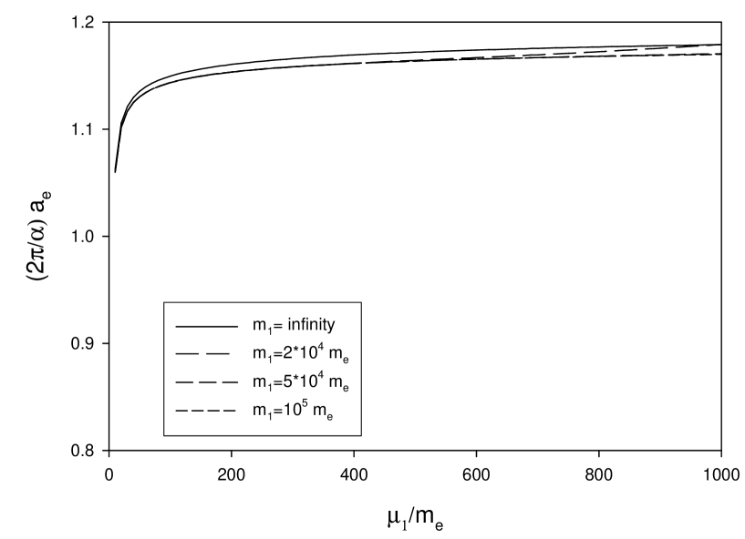
Figure 3: Same as Fig. 2, but with the second PV photon included, with a mass $\mu_{2}=\sqrt{2}\mu_{1}$, and the chiral symmetry is restored. The mass ratio is held fixed as $\mu_{1}$ and $\mu_{2}$ are varied.

Clearly, the dependence on the PV masses is greatly reduced. The value obtained for the anomalous moment differs from the leading-order Schwinger result Schwinger , and thus from the physical value, by 17%. Agreement at this level of accuracy is to be expected; the leading divergence in the normalization will not be cancelled until the truncation is relaxed to include two-photon states.

VI Summary

We have developed an improved Pauli–Villars regularization of light-front QED by establishing the correct chiral limit. Chiral symmetry is restored by the introduction of an additional Pauli–Villars photon. An application to the calculation of the anomalous magnetic moment of the electron shows much less dependence on the regulator masses, as can be seen in comparing results without and with the second PV field in Figs. 2 and 3, respectively.

The chiral condition on the coupling and mass of the second PV field is given in Eq. (49). It is of the same form as the constraint obtained earlier for Yukawa theory with three PV bosons ChiralSymYukawa ; bhm1 . Such a constraint should also be considered for the regularization of Yukawa theory with one PV boson and one PV fermion. This was not done in YukawaOneBoson or YukawaTwoBoson ; however, there none of the bosons is massless, and the anomalous moment is much less sensitive to constituent masses.

For less severe truncations, where more photons are allowed in Fock states, the number of PV photon flavors does not need to increase Paston . However, the chiral constraint will be more complicated. Fortunately, the corrections will be higher order in $\alpha$, and therefore should be small enough to be neglected.

Thus, we have a regularization scheme that can properly handle the one-photon truncation at finite PV electron mass and can be readily extended to higher truncations. The result for the anomalous moment in the one-photon truncation does differ by 17% from the experimental result, but this discrepancy is expected to be much reduced in the two-photon truncation which includes self-energy effects for the constituent electron.

Appendix A Gauge Condition

The gauge condition $\partial^{\mu}A_{i\mu}=0$ can be implemented as a projection for the positive frequency part GuptaBleuler ; GaugeCondition , with physical states $|\psi\rangle$ restricted by

$$\partial^{\mu}A_{i\mu}^{(+)}|\psi\rangle=\frac{1}{\sqrt{16\pi^{3}}}\int\frac{d\underline{k}}{\sqrt{k^{+}}}k^{\mu}a_{i\mu}(\underline{k})e^{-i\underline{k}\cdot\underline{x}}|\psi\rangle=0.$$ (59)

This restricts Fock-state expansions to physical polarizations in the following way GaugeCondition . Let $e_{\mu}^{(\lambda)}(\underline{k})$, with $\lambda=0,1,2,3$, be polarization vectors for a photon with four-momentum $k$, with the properties

$$e^{(\lambda)\mu}e_{\mu}^{(\lambda^{\prime})}=-\epsilon^{\lambda}\delta_{\lambda\lambda^{\prime}},$$ (60)

and

$$k^{\mu}e_{\mu}^{(\lambda)}=0,\;\;n^{\mu}e_{\mu}^{(\lambda)}=0,\;\;\lambda=1,2.$$ (61)

Here $\epsilon^{\mu}=(-1,1,1,1)$ is the metric signature, as in Sec. II, and $n$ is the timelike four-vector that reduces to $(1,0,0,0)$ in the frame where $\vec{k}_{\perp}=0$. We express the annihilation operator $a_{i\mu}$ in terms of these polarizations as

$$a_{i\mu}=\sum_{\lambda}e_{\mu}^{(\lambda)}a_{i}^{(\lambda)}.$$ (62)

The polarizations $\lambda=1,2$ are the physical transverse polarizations. The scalar and longitudinal polarizations may be chosen to be GaugeCondition

$$e^{(0)}=n\;\;\mbox{and}\;\;e^{(3)}(\underline{k})=\frac{k-(k\cdot n)n}{k\cdot n},$$ (63)

which satisfy the conditions (60). From these choices for $e^{(0)}$ and $e^{(3)}$, we have

$$k^{\mu}e_{\mu}^{(0)}=k\cdot n,\;\;k^{\mu}e_{\mu}^{(3)}=-k\cdot n,$$ (64)

and

$$k^{\mu}a_{i\mu}=k\cdot n(a_{i}^{(0)}-a_{i}^{(3)}).$$ (65)

Given this last result, it is convenient to define the linear combinations

$$a_{i}^{(\pm)}=(a_{i}^{(0)}\pm a_{i}^{(3)})/\sqrt{2}.$$ (66)

They are both null and satisfy the commutation relations

$$[a_{i}^{(\pm)}(\underline{k}),a_{i}^{(\pm)\dagger}(\underline{k}^{\prime})]=0,\;\;[a_{i}^{(\pm)}(\underline{k}),a_{i}^{(\mp)\dagger}(\underline{k}^{\prime})]=-(-1)^{i}\delta(\underline{k}-\underline{k}^{\prime}).$$ (67)

The restriction on physical states then reduces to

$$a_{i}^{(-)}|\psi\rangle=0.$$ (68)

Because $a_{i}^{(-)}$ commutes with all but $a_{i}^{(+)\dagger}$, the restriction (68) can be satisfied by removing from $|\psi\rangle$ all terms that contain $a_{i}^{(+)\dagger}$. This is accomplished by replacing all photon creation operators $a_{i\mu}^{\dagger}$ with the projected operator

$$\tilde{a}_{i\mu}^{\dagger}=\frac{1}{\sqrt{2}}(e_{\mu}^{(0)}-e_{\mu}^{(3)})a_{i}^{(-)\dagger}+\sum_{\lambda=1}^{2}e_{\mu}^{(\lambda)}a_{i}^{(\lambda)\dagger}.$$ (69)

Since the $a_{i}^{(-)\dagger}$ are null, only the physical polarizations contribute to expectation values of physical quantities.

The presence of photons created by $a_{i}^{(-)\dagger}$ corresponds to the residual gauge transformations GaugeCondition that satisfy $\partial^{\mu}A_{i\mu}=0$, where $A_{i\mu}\rightarrow A_{i\mu}+\partial_{\mu}\Lambda_{i}$ with $\Box\Lambda_{i}=0$. To see this, consider the expectation value GaugeCondition $\langle\psi|A_{i\mu}|\psi\rangle$, with $|\psi\rangle$ written as

$$|\psi\rangle=C_{0}|0\rangle+\int d\underline{q}C_{1}(\underline{q})a_{i}^{(-)\dagger}(\underline{q})|0\rangle+\cdots,$$ (70)

and transverse polarizations absent. In the expectation value only the $a_{i}^{(+)}$ and $a_{i}^{(+)\dagger}$ terms of $A_{i\mu}$ can contribute, as follows from the commutators in Eq. (67), and these terms give

$$\langle\psi|A_{i\mu}|\psi\rangle=-(-1)^{i}C_{0}^{*}\int\frac{d\underline{q}}{\sqrt{16\pi^{3}q^{+}}}C_{1}(\underline{q})e^{-iq\cdot x}\frac{1}{\sqrt{2}}(e_{\mu}^{(0)}(\underline{q})+e_{\mu}^{(3)}(\underline{q}))+\mbox{c.c.}$$ (71)

From (63) we have $e_{\mu}^{(0)}(\underline{q})+e_{\mu}^{(3)}(\underline{q})=2q_{\mu}/q^{+}$. The factor $q_{\mu}$ can be replaced by a partial derivative, leaving

$$\langle\psi|A_{i\mu}|\psi\rangle=\partial_{\mu}\Lambda_{i}(x),$$ (72)

with

$$\Lambda_{i}(x)=-i(-1)^{i}C_{0}^{*}\int\frac{d\underline{q}}{(2\pi q^{+})^{3/2}}C_{1}(\underline{q})e^{-iq\cdot x}+\mbox{c.c.}$$ (73)

Since $q$ is null, $\Box\Lambda_{i}=0$. Thus, the contribution from the unphysical polarizations is a pure gauge term consistent with the residual gauge symmetry. A choice of wave function for the minus polarization corresponds to a choice for the residual gauge.

Appendix B Proof of $\bar{J}=M^{2}\bar{I}_{0}$

Here we give a proof of the identity $\bar{J}=M^{2}\bar{I}_{0}$ for the integrals $\bar{I}_{0}$ and $\bar{J}$ defined in (33) and (34), respectively. It involves an interesting coordinate transformation that might have broader application.

We write the integrals in terms of their individual Fock-sector contributions as

$$\bar{I}_{0} = -\frac{1}{16\pi^{2}}\sum_{jl}(-1)^{j+l}\xi_{l}I_{0jl},$$ (74)

$$\bar{J} = -\frac{1}{16\pi^{2}}\sum_{jl}(-1)^{j+l}\xi_{l}J_{jl},$$

with

$$I_{0jl} \equiv \int\frac{dydk_{\perp}^{2}}{y}\frac{1}{\frac{m_{j}^{2}+k_{\perp}^{2}}{1-y}+\frac{\mu_{l}^{2}+k_{\perp}^{2}}{y}-M^{2}},$$ (75)

$$J_{jl} \equiv \int\frac{dydk_{\perp}^{2}}{y(1-y)^{2}}\frac{m_{j}^{2}+k_{\perp}^{2}}{\frac{m_{j}^{2}+k_{\perp}^{2}}{1-y}+\frac{\mu_{l}^{2}+k_{\perp}^{2}}{y}-M^{2}}.$$

For the $J$ integrals, we replace $y$ with a new variable $x$ defined by

$$x=(1-y)\frac{\mu_{l}^{2}+k_{\perp}^{2}}{m_{j}^{2}y+\mu_{l}^{2}(1-y)+k_{\perp}^{2}}.$$ (76)

It also ranges between 0 and 1, though in the reverse order relative to $y$, and has the remarkable property that

$$\frac{m_{j}^{2}+k_{\perp}^{2}}{1-y}+\frac{\mu_{l}^{2}+k_{\perp}^{2}}{y}=\frac{m_{j}^{2}+k_{\perp}^{2}}{1-x}+\frac{\mu_{l}^{2}+k_{\perp}^{2}}{x},$$ (77)

even though $x$ and $y$ are clearly not equal and are not even linearly related.

With this change of variable, the $J$ integrals become

$$J_{jl}=\int\frac{dxdk_{\perp}^{2}}{x}\frac{m_{j}^{2}x+\mu_{l}^{2}(1-x)+k_{\perp}^{2}}{x(1-x)}\frac{1}{\frac{m_{j}^{2}+k_{\perp}^{2}}{1-x}+\frac{\mu_{l}^{2}+k_{\perp}^{2}}{x}-M^{2}}.$$ (78)

The middle factor can be written as

$$\frac{m_{j}^{2}x+\mu_{l}^{2}(1-x)+k_{\perp}^{2}}{x(1-x)}=\frac{m_{j}^{2}+k_{\perp}^{2}}{1-x}+\frac{\mu_{l}^{2}+k_{\perp}^{2}}{x}-M^{2}+M^{2},$$ (79)

so that we obtain

$$J_{jl}=\int\frac{dxdk_{\perp}^{2}}{x}+\int\frac{dxdk_{\perp}^{2}}{x}\frac{M^{2}}{\frac{m_{j}^{2}+k_{\perp}^{2}}{1-x}+\frac{\mu_{l}^{2}+k_{\perp}^{2}}{x}-M^{2}}.$$ (80)

This last result shows that $J_{jl}$ is just $M^{2}I_{0jl}$ plus an (infinite) constant. Since the constant cancels in the sum over PV particles $\sum_{jl}(-1)^{j+l}\xi_{l}$, we have the desired identity of $\bar{J}=M^{2}\bar{I}_{0}$.

References

- (1) W. Pauli and F. Villars, Rev. Mod. Phys. 21, 434 (1949).
- (2) S.J. Brodsky, J.R. Hiller, and G. McCartor, Phys. Rev. D 58, 025005 (1998).
- (3) S.J. Brodsky, J.R. Hiller, and G. McCartor, Phys. Rev. D 60, 054506 (1999).
- (4) S.J. Brodsky, J.R. Hiller, and G. McCartor, Phys. Rev. D 64, 114023 (2001), hep-ph/0107038.
- (5) S.J. Brodsky, J.R. Hiller, and G. McCartor, Ann. Phys. 296, 406 (2002), hep-th/0107246.
- (6) S.J. Brodsky, J.R. Hiller, and G. McCartor, Ann. Phys. 305, 266 (2003), hep-th/0209028.
- (7) S.J. Brodsky, V.A. Franke, J.R. Hiller, G. McCartor, S.A. Paston, and E.V. Prokhvatilov, Nucl. Phys. B 703, 333 (2004), hep-ph/0406325.
- (8) S.J. Brodsky, J.R. Hiller, and G. McCartor, Ann. Phys. 321, 1240 (2006), hep-ph/0508295.
- (9) P.A.M. Dirac, Rev. Mod. Phys. 21, 392 (1949).
- (10) For reviews, see M. Burkardt, Adv. Nucl. Phys. 23, 1 (2002); S.J. Brodsky, H.-C. Pauli, and S.S. Pinsky, Phys. Rep. 301, 299 (1998).
- (11) For reviews, see M. Creutz, L. Jacobs and C. Rebbi, Phys. Rep. 93, 201 (1983); J.B. Kogut, Rev. Mod. Phys. 55, 775 (1983); I. Montvay, ibid. 59, 263 (1987); A.S. Kronfeld and P.B. Mackenzie, Ann. Rev. Nucl. Part. Sci. 43, 793 (1993); J.W. Negele, Nucl. Phys. A553, 47c (1993); K.G. Wilson, Nucl. Phys. B (Proc. Suppl.) 140, 3 (2005); J.M. Zanotti, PoS LAT2008, 007 (2008).
- (12) C.D. Roberts and A.G. Williams, Prog. Part. Nucl. Phys. 33, 477 (1994); P. Maris and C.D. Roberts, Int. J. Mod. Phys. E12, 297 (2003); P.C. Tandy, Nucl. Phys. B (Proc. Suppl.) 141, 9 (2005).
- (13) S.A. Paston and V.A. Franke, Theor. Math. Phys. 112, 1117 (1997) [Teor. Mat. Fiz. 112, 399 (1997)], hep-th/9901110; S.A. Paston, V.A. Franke, and E.V. Prokhvatilov, Theor. Math. Phys. 120, 1164 (1999) [Teor. Mat. Fiz. 120, 417 (1999)], hep-th/0002062.
- (14) R.J. Perry, A. Harindranath, and K.G. Wilson, Phys. Rev. Lett. 65, 2959 (1990); R.J. Perry and A. Harindranath, Phys. Rev. D 43, 4051 (1991).
- (15) T. Kinoshita and M. Nio, Phys. Rev. Lett. 90, 021803 (2003); V.W. Hughes and T. Kinoshita, Rev. Mod. Phys. 71, S133 (1999).
- (16) C. Bouchiat, P. Fayet, and N. Sourlas, Lett. Nuovo Cim. 4, 9 (1972); S.-J. Chang and T.-M. Yan, Phys. Rev. D 7, 1147 (1973); M. Burkardt and A. Langnau, Phys. Rev. D 44, 1187 (1991).
- (17) S.J. Brodsky and S.D. Drell, Phys. Rev. D 22, 2236 (1980).
- (18) J.R. Hiller and S.J. Brodsky, Phys. Rev. D 59, 016006 (1998).
- (19) V. A. Karmanov, J. F. Mathiot and A. V. Smirnov, Phys. Rev. D 75, 045012 (2007); J. F. Mathiot, V. A. Karmanov and A. V. Smirnov, Nucl. Phys. Proc. Suppl. 161, 160 (2006).
- (20) D. Bernard, Th. Cousin, V.A. Karmanov, and J.-F. Mathiot, Phys. Rev. D 65, 025016 (2001).
- (21) H.-C. Pauli and S.J. Brodsky, Phys. Rev. D 32, 1993 (1985); 32, 2001 (1985).
- (22) G.P. Lepage and S.J. Brodsky, Phys. Rev. D 22, 2157 (1980).
- (23) S.N. Gupta, Proc. Phys. Soc. (London) A63, 681 (1950); K. Bleuler, Helv. Phys. Acta 23, 567 (1950).
- (24) N.N. Bogoliubov and D.V. Shirkov, Introduction to the Theory of Quantized Fields, (Interscience, New York, 1959); S. Schweber, An Introduction to Relativistic Quantum Field Theory, (Harper & Row, New York, 1961); C. Itzykson and J.-B. Zuber, Quantum Field Theory, (McGraw–Hill, New York, 1980).
- (25) S.J. Brodsky, R. Roskies, and R. Suaya, Phys. Rev. D 8, 4574 (1973).
- (26) J. Schwinger, Phys. Rev. 73, 416 (1948); 76, 790 (1949).