A Time-Periodic Lyapunov Approach for Motion Planning of
Controllable Driftless Systems on $\mbox{SU}(n)$

Abstract

For a right-invariant and controllable driftless system on $\mbox{SU}(n)$, we consider a time-periodic reference trajectory along which the linearized control system generates $\mathfrak{su}(n)$: such trajectories always exist and constitute the basic ingredient of Coron’s Return Method. The open-loop controls that we propose, which rely on a left-invariant tracking error dynamics and on a fidelity-like Lyapunov function, are determined from a finite number of left-translations of the tracking error and they assure global asymptotic convergence towards the periodic reference trajectory. The role of these translations is to avoid being trapped in the critical region of this Lyapunov-like function. The convergence proof relies on a periodic version of LaSalle’s invariance principle and the control values are determined by numerical integration of the dynamics of the system. Simulations illustrate the obtained controls for $n=4$ and the generation of the C–NOT quantum gate.

I INTRODUCTION

Consider the right-invariant driftless system

$$\dot{X}=\sum_{k=1}^{m}u_{k}H_{k}X,\hskip 12.0ptX(0)=I,$$ (1)

where $X\in M^{n}$ is the state, $M^{n}$ is the Banach space of square $n\times n$ matrices with complex entries endowed with the Euclidean norm, $H=\{H_{1},\dots,H_{m}\}\subset\mathfrak{su}(n)$, $u_{k}\in\mathbb{R}$ are the controls, and $I$ is the identity matrix of $M^{n}$. The periodic motion planning problem for this system is formulated as follows. Given a goal state $X_{\infty}\in\mbox{SU}(n)$ and $T>0$, find a smooth periodic reference trajectory $X_{r}$: $\mathbb{R}_{+}\rightarrow\mbox{SU}(n)$ of period $T$, with $X_{r}(0)=X_{\infty}$, and determine continuous open-loop controls $u_{k}$: $\mathbb{R}_{+}\rightarrow\mathbb{R}$, for $1\leq k\leq m$, in a manner that the tracking error between the trajectory $X$: $\mathbb{R}_{+}\rightarrow\mbox{SU}(n)$ of (1) and $X_{r}$ converges to zero as $t\rightarrow\infty$, that is, $\lim_{t\rightarrow\infty}[X(t)-X_{r}(t)]=0$.

We remark that there is no loss of generality in assuming that $X(0)=I$ in (1). Indeed, since system (1) is right-invariant, if $(X(t),(u_{1}(t),\dots,u_{m}(t)))$, for $t\in\mathbb{R}_{+}$, is a solution of (1) with $X(0)=I$, then $(X(t)X_{0},(u_{1}(t),\dots,u_{m}(t)))$, for $t\in\mathbb{R}_{+}$, is a solution of (1) with initial condition $X(0)=X_{0}\in\mbox{SU}(n)$. Therefore, if the periodic motion planning problem has been solved for system (1) with $X(0)=I$, it is straightforward to show that it will also be solved for (1) with $X(0)=X_{0}\in\mbox{SU}(n)$.

The main result of this paper is the determination of a solution for the periodic motion planning problem. This is established by Theorem 2 in Section 2, whose only assumption is that system (1) regular, in the sense of Definition 1 in Section 2. The results of Coron’s Return Method show that such condition is always met in case the system is controllable on $\mbox{SU}(n)$ (see Remark 2 in Section 2). Loosely speaking, by finding an appropriate reference trajectory $X_{r}$, using the time-dependent change of coordinates $Z=Z(X,t)=X^{\dagger}X_{r}(t)$, which corresponds to the tracking error on the group $\mbox{SU}(n)$, and defining an adequate “feedback”, we determine an algorithm that obtains, in a finite number of steps, continuous open-loops controls $u_{k}$, for every $1\leq k\leq m$, which assure that the tracking error $X-X_{r}$ converges to zero as $t\rightarrow\infty$. This algorithm relies on Lyapunov-like convergence results inspired in the periodic version of LaSalle’s invariance principle presented in [11], and in the ad-condition stabilization method of [6]. In a certain sense, we have used the real part of the trace of the left-invariant tracking error $Z$ as a Lyapunov-like function, that is, $V(Z)=\Re(tr(Z))$. In the case of quantum systems, $V$ can then be seen as a fidelity-like Lyapunov function.

The problem of steering a quantum system from a given initial state to an arbitrary final state, which can be regarded as a particular case of the periodic motion planning problem here formulated, has recently been treated in [8] using a flatness-based approach and in the book [4] (see also the references therein), where many quantum control techniques used in the literature are grouped together and explained in detail, such as Lyapunov-based methods, optimal control and decompositions of $\mbox{SU}(n)$. Our Lyapunov-like approach has no restrictions on the goal state $X_{\infty}\in\mbox{SU}(n)$ and on $n$, as long as system (1) is regular.

The layout of the paper is as follows. Section 2 is entirely dedicated to the proof of Theorem 2 mentioned above. Simulations illustrate in Section 3 the generation of the Controlled-NOT (C–NOT) gate for a quantum system with $n=4$. Appendix presents the proof of the important convergence result of Theorem 1 in Section 2.

II Main Result

Based on (1), we define the reference system

$$\dot{X_{r}}=\sum_{k=1}^{m}u^{r}_{k}H_{k}X_{r},\hskip 12.0ptX_{r}(0)=X_{\infty}\in\mbox{SU}(n),$$ (2)

where $X_{r}\in M^{n}$ and the smooth time functions $u^{r}_{k}$: $\mathbb{R}\rightarrow\mathbb{R}$ are still to be specified.

Definition 1

System (1) is said to be regular when, given $T>0$, there exist smooth periodic functions $u^{T}_{k}$: $\mathbb{R}\rightarrow\mathbb{R}$ of period $T$, for all $1\leq k\leq m$, such that the solution $X^{T}_{r}$: $\mathbb{R}_{+}\rightarrow\mbox{SU}(n)$ of (2), with $X^{T}_{r}(0)=I$ and $u^{r}_{k}=u^{T}_{k}$, is also periodic of period $T$ and satisfies

$$\mbox{span}\{B^{j}_{k}(0),1\leq k\leq m,j\in\mathbb{N}\}=\mathfrak{su}(n),$$ (3)

where $\mathbb{N}$ is the set of natural numbers (including zero), $A(t)=\sum_{k=1}^{m}u^{T}_{k}(t)H_{k}\in\mathfrak{su}(n)$, $B^{0}_{k}(t)=H_{k}X^{T}_{r}(t)$, $B^{j+1}_{k}(t)=-A(t)B^{j}_{k}(t)+\dot{B}^{j}_{k}(t)$, $1\leq k\leq m$, $j\in\mathbb{N}$, $t\in\mathbb{R}$.

Remark 1

Note that $A$: $\mathbb{R}\rightarrow\mathfrak{su}(n)$, $B^{j}_{k}$, $\dot{B}^{j}_{k}$: $\mathbb{R}\rightarrow M^{n}$ are smooth and also have period $T$, for every $1\leq k\leq m$, $j\in\mathbb{N}$. Hence, they are bounded mappings.

Remark 2

Note that the linearized control system of (2) (or of (1)) along the trajectory $(X_{r}^{T},(u_{1}^{T},\dots,u_{m}^{T}))$ is given by $\dot{X}_{r}^{\ell}=A(t)X_{r}^{\ell}+\sum_{k=1}^{m}w_{k}B^{0}_{k}(t)$, $w_{k}\in\mathbb{R}$. Based on Coron’s Return Method (see [2], [3]), it can be shown that (1) is regular in case $\mbox{Lie}(H)=\mathfrak{su}(n)$. We recall that (1) is controllable on $\mbox{SU}(n)$ if and only if $\mbox{Lie}(H)=\mathfrak{su}(n)$ [1].

For simplicity, we shall assume throughout this paper that system (1) is regular, that $T>0$ has been fixed and that the functions $u^{r}_{k}$ in (2) were specified accordingly, that is, $u^{r}_{k}=u^{T}_{k}$, for $1\leq k\leq m$. Moreover, we also assume that the goal state $X_{\infty}\in\mbox{SU}(n)$ is fixed. Define $X_{r}$: $\mathbb{R}\rightarrow\mbox{SU}(n)$ as $X_{r}=X^{T}_{r}X_{\infty}$. Note that $X_{r}$ is the solution of (2) with $X_{r}(0)=X_{\infty}$ and that $X_{r}$ also has period $T$. It will be shown afterwards that $X_{r}$ can indeed be used as a reference trajectory. We also adopt the following notations. The imaginary unit of $\mathbb{C}$ is denoted by $\imath$ and if $z\in\mathbb{C}$, then $\Re(z)$ is its real part and $\Im(z)$ its imaginary part.

It is straightforward to verify from (1) and (2) that the time-dependent change of coordinates

$$Z=Z(t,X)=X^{{\dagger}}X_{r}(t),\hskip 12.0pt\mbox{ for all }(t,X)\in\mathbb{R}\times M^{n},$$

along with the time-varying control shift

$$v_{k}\triangleq u_{k}^{r}(t)-u_{k}=u_{k}^{T}(t)-u_{k},\hskip 12.0pt\mbox{ for all }t\in\mathbb{R},\;1\leq k\leq m,$$

determine the left-invariant “closed-loop system”

$$\dot{Z}=ZX^{\dagger}_{r}(t)\sum_{k=1}^{m}v_{k}H_{k}X_{r}(t),\hskip 8.0ptZ(0)=X_{\infty}\in\mbox{SU}(n),$$ (4)

for all $(t,Z)\in\mathbb{R}\times M^{n}$. If we can find continuous functions $v_{k}$: $\mathbb{R}_{+}\rightarrow\mathbb{R}$, for each $1\leq k\leq m$, such that

$$\lim_{t\rightarrow\infty}Z(t)=\lim_{t\rightarrow\infty}X^{{\dagger}}(t)X_{r}(t)=I,$$ (5)

where $Z$: $\mathbb{R}_{+}\rightarrow\mbox{SU}(n)$ is the solution of system (4) and $X$: $\mathbb{R}_{+}\rightarrow\mbox{SU}(n)$ is the solution of system (1) with the continuous open-loop controls

$$u_{k}(t)=u^{T}_{k}(t)-v_{k}(t),\hskip 12.0pt\mbox{ for all }t\in\mathbb{R}_{+},\;1\leq k\leq m,$$

it is then clear that

$$\lim_{t\rightarrow\infty}[X(t)-X_{r}(t)]=0,$$ (6)

thus solving the periodic motion planning problem.

Let $V$: $M^{n}\rightarrow\mathbb{R}$ be defined by

$$V(X)=\Re(tr(X)),\hskip 12.0pt\mbox{ for all }X\in M^{n},$$ (7)

and consider the auxiliar system

$$\dot{W}=WX^{\dagger}_{r}(t)\sum_{k=1}^{m}f_{k}a_{k}(t,W)H_{k}X_{r}(t),$$ (8)

where $(t,W)\in\mathbb{R}\times M^{n}$, $f_{k}\neq 0$ is a fixed real number, $1\leq k\leq m$, and

$$a_{k}(t,W)=f_{k}\mathrm{V}(WX^{{\dagger}}_{r}(t)H_{k}X_{r}(t)).$$ (9)

Notice that the “closed-loop” system (4) with “feedbacks” $v_{k}=f_{k}a_{k}(t,Z)$ is nothing but the auxiliar system (8)–(9). Note also that $V$ in (7) is linear and that, for $X\in\mbox{SU}(n)$, we have $-n\leq V(X)\leq n$ and $V(X)=n$ if and only if $X=I$. Furthermore, by construction, $\dot{\mathrm{V}}(t,W)=\sum_{k=1}^{m}a_{k}(t,W)^{2}\geq 0$, for all $(t,W)\in\mathbb{R}\times M^{n}$.

In what follows, we shall show how the next theorem, which is a Lyapunov-like convergence result for the auxiliar system with Lyapunov-like function $V(W)=\Re(tr(W))$, and whose proof is deferred to Appendix, determines continuous functions $v_{k}$: $\mathbb{R}_{+}\rightarrow\mathbb{R}$, for $1\leq k\leq m$, such that (5) is satisfied for the “closed-loop” system (4). We remark that the properties of $V$ stated above are essential in the proof. Our approach to solve the periodic motion planning problem is then summarized in Theorem 2.

Theorem 1

Consider the set

$$G=\{ x\in\mathbb{R}:x=\sum_{i=1}^{n}\Re(\lambda_{i}),\mbox{ for some }\lambda_{i}\in\mathbb{C}\mbox{ such}$$

$$\mbox{that }|\lambda_{i}|=1,\prod_{i=1}^{n}\lambda_{i}=1,\Im(\lambda_{1})=\dots=\Im(\lambda_{n})\}.$$

Then, $G$ is a finite set, $n\in G$ and $n=\max(G)$. Furthermore, letting $\delta$ be the maximal element of the set $G\setminus\{n\}$, we have that, for all $q=(t_{0},W_{t_{0}})\in\mathbb{R}\times\mbox{SU}(n)$,

$$V(W_{t_{0}})>\delta\Rightarrow\lim_{t\rightarrow\infty}W_{q}(t)=I,$$

where $W_{q}$: $\mathbb{R}\rightarrow\mbox{SU}(n)$ is the solution of (8)–(9) with initial condition $W_{q}(t_{0})=W_{t_{0}}$.

Suppose that $V(X_{\infty})>\delta$. In Theorem 1, we choose $q=(0,X_{\infty})\in\mathbb{R}\times\mbox{SU}(n)$. Therefore, $\lim_{t\rightarrow\infty}W_{q}(t)=I$. Hence, the smooth “feedbacks” $v_{k}$: $\mathbb{R}_{+}\rightarrow\mathbb{R}$ defined as

$$v_{k}(t)\triangleq f_{k}a_{k}(t,Z(t))=f_{k}^{2}\mathrm{V}(X^{\dagger}(t)H_{k}X_{r}(t)),$$

for $t\in\mathbb{R}_{+}$, $1\leq k\leq m$, assure that $Z(t)=W_{q}(t)$, for $t\in\mathbb{R}_{+}$. Indeed, compare (4) with (8)–(9). Thus, (5) holds.

Now, assume that $V(X_{\infty})\leq\delta$. For this case, based on continuity arguments, we determine an adequate (continuous) path from $X_{\infty}$ to $I$ which, in a certain sense, reduces the problem to the situation where $V(X_{\infty})>\delta$. In order to achieve this, the main idea is to find a path $\overline{Z}$: $[0,1]\rightarrow\mbox{SU}(n)$, with $\overline{Z}(0)=X_{\infty}$ and $\overline{Z}(1)=I$, and obtain $0=\theta_{0}<\theta_{1}<\dots<\theta_{N-1}<\theta_{N}=1$, such that $V(\overline{Z}(\theta_{\ell+1})^{\dagger}\overline{Z}(\theta_{\ell}))>\delta$, for all $0\leq\ell\leq N-1$. It thus follows from Theorem 1 that, for $1\leq\ell\leq N$, $\lim_{t\rightarrow\infty}\overline{Z}(\theta_{\ell})W_{\ell}(t)=\overline{Z}(\theta_{\ell})$, where $W_{\ell}$: $\mathbb{R}\rightarrow\mbox{SU}(n)$ is the solution of (8)–(9) with initial condition $W_{\ell}(T_{\ell})=\overline{Z}(\theta_{\ell})^{\dagger}\overline{Z}(\theta_{\ell-1})\in\mbox{SU}(n)$, where $0=T_{1}<\dots<T_{N+1}$ are such that $W_{\ell}(T_{\ell+1})\thickapprox I$. Loosely speaking, we then “glue” together the left-translations $\overline{Z}(\theta_{1})W_{1},\dots,\overline{Z}(\theta_{N})W_{N}$ in an appropriate manner in order to define a continuous solution $(Z(t),(v_{1}(t),\dots,v_{m}(t)))$, for $t\in\mathbb{R}_{+}$, of system (4) that satisfies (5). We remark that, for every $1\leq\ell\leq N$, it is as if we were in the case $V(X_{\infty})>\delta$. In the sequel, we formalise these arguments in detail and determine an algorithm which obtains, in $N$ steps, continuous functions $v_{k}$: $\mathbb{R}_{+}\rightarrow\mathbb{R}$, for $1\leq k\leq m$, such that (5) holds.

It is a standard result that any $X_{\infty}\in\mbox{SU}(n)$ can be written as $X_{\infty}=M^{\dagger}\mbox{diag}(\exp{\imath\lambda_{1}},\dots,\exp{\imath\lambda_{n}})M$, where $M$ is a unitary matrix, $\lambda_{1},\dots,\lambda_{n}\in\mathbb{R}$ and $\sum^{n}_{i=1}\lambda_{i}=0$. Consider the path $\overline{Z}$: $[0,1]\rightarrow\mbox{SU}(n)$ from $X_{\infty}$ to $I$ defined by

$$\overline{Z}(\theta)=M^{\dagger}\mbox{diag}(\exp{\imath\lambda_{1}(1-\theta)},\dots,\exp{\imath\lambda_{n}(1-\theta)})M,$$

for all $\theta\in[0,1]$. Let $a,b\in[0,1]$. Hence, $\overline{Z}(b)^{\dagger}\overline{Z}(a)=M^{\dagger}\mbox{diag}(\exp{\imath\lambda_{1}(b-a)},\dots,\exp{\imath\lambda_{n}(b-a)})M$ and therefore $V(\overline{Z}(b)^{\dagger}\overline{Z}(a))=\sum_{j=1}^{n}\cos(\lambda_{j}(b-a))$. Since the function $\gamma$: $[0,1]\rightarrow\mathbb{R}$ defined by $\gamma(\theta)=\sum_{j=1}^{n}\cos(\lambda_{j}\theta)$, for all $\theta\in[0,1]$, is continuous with $\gamma(0)=n$, there exists $\nu>0$ such that $\gamma(\theta)>\delta$ in case $|\theta|<\nu$, for all $\theta\in[0,1]$ (indeed, choose $\epsilon=n-\delta>0$). Hence, $V(\overline{Z}(b)^{\dagger}\overline{Z}(a))>\delta$ whenever $|b-a|<\nu$, for all $a,b\in[0,1]$, and there exists a non-zero $\eta\in\mathbb{N}$ such that, for all $N\geq\eta$,

$$V(\overline{Z}_{\ell+1}^{\dagger}\overline{Z}_{\ell})=\sum_{j=1}^{n}\cos(\lambda_{j}\Delta)>\delta,$$ (10)

for all $0\leq\ell\leq N-1$, where $\overline{Z}_{\ell}=\overline{Z}(\theta_{\ell})$, $\theta_{\ell}=\ell\Delta$, for every $0\leq\ell\leq N$, with $\Delta=1/N$. Note that $\overline{Z}_{0}=\overline{Z}(0)=X_{\infty}$ and $\overline{Z}_{N}=\overline{Z}(1)=I$. Let $N\geq\eta$ and consider the continuous function $\beta$: $M^{n}\times M^{n}\rightarrow\mathbb{R}$ defined by $\beta(X,Y)=V(Y^{\dagger}X)$, for all $(X,Y)\in M^{n}\times M^{n}$. Since $\mbox{SU}(n)\times\mbox{SU}(n)$ is compact, $\beta|(\mbox{SU}(n)\times\mbox{SU}(n))$ is uniformly continuous. Therefore, by (10), there exists $\mu>0$ such that, for all $X\in\mbox{SU}(n)$ and $0\leq\ell\leq N-1$, we have

$$\|X-\overline{Z}_{\ell}\|<\mu\Rightarrow V(\overline{Z}_{\ell+1}^{\dagger}X)>\delta$$ (11)

(indeed, choose $\epsilon=\sum_{j=1}^{n}\cos(\lambda_{j}\Delta)-\delta>0$ and consider the sup norm on $M^{n}\times M^{n}$). The aforementioned algorithm is described below. Recall that $\overline{Z}_{0}=X_{\infty}$ and $\overline{Z}_{N}=I$.

Algorithm 1

Let $X_{\infty}\in\mbox{SU}(n)$. Choose any non-zero $N\in\mathbb{N}$ in a manner that (10) holds. Define $T_{1}=0$ and $W_{0}(T_{1})=I$. For every $1\leq\ell\leq N-1$, choose a real number $T_{\ell+1}>T_{\ell}$ such that $V(\overline{Z}_{\ell+1}^{\dagger}\overline{Z}_{\ell}W_{\ell}(T_{\ell+1}))>\delta$, where $W_{\ell}$: $\mathbb{R}\rightarrow\mbox{SU}(n)$ is the solution of the auxiliar system (8)–(9) with initial condition $W_{\ell}(T_{\ell})=\overline{Z}_{\ell}^{\dagger}\overline{Z}_{\ell-1}W_{\ell-1}(T_{\ell})\in\mbox{SU}(n)$. Define

$$Z(t) =\overline{Z}_{\ell}W_{\ell}(t)\in\mbox{SU}(n),\,\hskip 57.0pt\mbox{for }t\in[T_{\ell},T_{\ell+1}),$$

$$v_{k}(t) =f_{k}a_{k}(t,W_{\ell}(t))\in\mathbb{R},\,1\leq k\leq m,\,\mbox{for }t\in[T_{\ell},T_{\ell+1}).$$

If $T_{N}>T_{N-1}$ has been chosen as above, define

$$Z(t) =W_{N}(t)\in\mbox{SU}(n), \mbox{ for }t\geq T_{N},$$

$$v_{k}(t) =f_{k}a_{k}(t,W_{N}(t))\in\mathbb{R},\hskip 4.0pt1\leq k\leq m, \mbox{ for }t\geq T_{N},$$

where $W_{N}$: $\mathbb{R}\rightarrow\mbox{SU}(n)$ is the solution of (8)–(9) with initial condition $W_{N}(T_{N})=\overline{Z}_{N-1}W_{N-1}(T_{N})\in\mbox{SU}(n)$.          $\blacksquare$

Some remarks are in order. First of all, from the reasoning preceding Algorithm 1, we know that there always exists some non-zero $N\in\mathbb{N}$ such that (10) is true. Furthermore, Theorem 1 and property (11) assure that $T_{\ell+1}>T_{\ell}$ can always be chosen as required in the algorithm, for every $1\leq\ell\leq N-1$. It is also clear that $(Z(t),(v_{1}(t),\dots,v_{m}(t)))$, for $t\in\mathbb{R}_{+}$, determined by the algorithm is a continuous solution of the “closed-loop” system (4). Indeed, compare (4) with (8)–(9). Finally, since $V(\overline{Z}_{N}^{\dagger}\overline{Z}_{N-1}W_{N-1}(T_{N}))=V(\overline{Z}_{N-1}W_{N-1}(T_{N}))>\delta$, Theorem 1 implies that $\lim_{t\rightarrow\infty}W_{N}(t)=I$. However, $Z(t)=W_{N}(t)$, for $t\geq T_{N}$. Therefore, the continuous functions $v_{k}$: $\mathbb{R}_{+}\rightarrow\mathbb{R}$ determined by Algorithm 1 are such that (5) is satisfied. We have thus shown our main result:

Theorem 2

Assume that system (1) is regular, in the sense of Definition 1. Given $X_{\infty}\in\mbox{SU}(n)$, $T>0$ and “feedback gains” $f_{k}^{2}>0$, consider $X_{r}^{T}$: $\mathbb{R}\rightarrow\mbox{SU}(n)$ and $u_{k}^{T}$: $\mathbb{R}\rightarrow\mathbb{R}$ as in Definition 1, for $1\leq k\leq m$. Define $X_{r}=X_{r}^{T}X_{\infty}$. Then, there exist continuous open-loop controls $u_{k}$: $\mathbb{R}_{+}\rightarrow\nolinebreak\mathbb{R}$, for $1\leq k\leq m$, such that (6) is satisfied. In other words, the periodic motion planning problem always has a solution when (1) is regular. More precisely, if $V(X_{\infty})>\delta$, where $\delta$ is as in Theorem 1, then the smooth open-loop controls $u_{k}(t)=u_{k}^{T}(t)-f_{k}^{2}\mathrm{V}(X^{\dagger}(t)H_{k}X_{r}(t))$, obtained by numerical integration, for $t\in\mathbb{R}_{+}$, $1\leq k\leq m$, assure that (6) holds. Otherwise, in case $V(X_{\infty})\leq\delta$, then by following Algorithm 1 we determine continuous functions $v_{k}$: $\mathbb{R}_{+}\rightarrow\mathbb{R}$, for $1\leq k\leq m$, such that the corresponding continuous open-loop controls $u_{k}(t)=u_{k}^{T}(t)-v_{k}(t)$, for $t\in\mathbb{R}_{+}$, assure that (6) is satisfied.

III QUANTUM MECHANICAL EXAMPLE

After some approximations, an appropriate change of coordinates, scalings and simplifications, a controlled quantum system consisting of two coupled spin-$\frac{1}{2}$ particles with Heisenberg interaction and driven by an external electromagnetic field, can be modeled as [4]

$$\dot{Y}=(D+D_{x}u_{x}+D_{y}u_{y}+D_{z}u_{z})Y,\hskip 12.0ptY(0)=I,$$ (12)

where $Y\in M^{4}$ ($n=4$), the controls $u_{x}$, $u_{y}$, $u_{z}\in\mathbb{R}$ are the $x$, $y$, $z$ components of the electromagnetic field, respectively, $D=\mbox{diag}(3\imath,-\imath,-\imath,-\imath)$, $D_{x}=H^{R}_{14}-3H^{R}_{23}$, $D_{y}=H^{R}_{13}+3H^{R}_{24}$, $D_{z}=H^{R}_{12}-3H^{R}_{34}\in\mathfrak{su}(4)$, and $H^{R}_{ij}=(h^{R,ij}_{k\ell})$, $H^{I}_{ij}=(h^{I,ij}_{k\ell})\in\mathfrak{su}(4)$ are the matrices with entries

$$h^{R,ij}_{ij}=1,\hskip 4.0pth^{R,ij}_{ji}=-1,\hskip 4.0pth^{R,ij}_{k\ell}=0,\hskip 12.0pt\mbox{ for }k,\ell\neq i,j,\vskip 6.0pt plus 2.0pt minus 2.0pt$$

$$h^{I,ij}_{ij}=h^{I,ij}_{ji}=\imath,\hskip 31.0pth^{I,ij}_{k\ell}=0,\hskip 14.0pt\mbox{ for }k,\ell\neq i,j,$$

respectively, for all $1\leq i<j\leq n$.

Now, in order to remove the drift term $DY$ in (12), we define, as usual, the time-dependent change of coordinates $X=\Phi(t,Y)=e^{-Dt}Y$, for all $(t,Y)\in\mathbb{R}\times M^{4}$. In these coordinates, (12) is described as

$$\dot{X}=(C_{x}u_{x}+C_{y}u_{y}+C_{z}u_{z})X,\hskip 12.0ptX(0)=I,$$ (13)

where

$$\begin{array}[]{l}C_{x}=e^{-Dt}D_{x}e^{Dt}=\left(\begin{array}[]{rrrl}0&0&0&e^{-\imath 4t}\\ 0&0&-3&0\\ 0&3&0&0\\ -e^{\imath 4t}&0&0&0\\ \end{array}\right),\vskip 6.0pt plus 2.0pt minus 2.0pt\\ C_{y}=e^{-Dt}D_{y}e^{Dt}=\left(\begin{array}[]{rrlr}0&0&e^{-\imath 4t}&0\\ 0&0&0&3\\ -e^{\imath 4t}&0&0&0\\ 0&-3&0&0\\ \end{array}\right),\vskip 6.0pt plus 2.0pt minus 2.0pt\\ C_{z}=e^{-Dt}D_{z}e^{Dt}=\left(\begin{array}[]{rlrr}0&e^{-\imath 4t}&0&0\\ -e^{\imath 4t}&0&0&0\\ 0&0&0&-3\\ 0&0&3&0\\ \end{array}\right),\end{array}$$

for all $t\in\mathbb{R}$. We choose the real controls $u_{x}$, $u_{y}$, $u_{z}$ as

$$\begin{array}[]{l}u_{x}=(u_{1}+\imath u_{2})e^{\imath 4t}+(u_{1}-\imath u_{2})e^{-\imath 4t},\vskip 6.0pt plus 2.0pt minus 2.0pt\\ u_{y}=(u_{3}+\imath u_{4})e^{\imath 4t}+(u_{3}-\imath u_{4})e^{-\imath 4t},\vskip 6.0pt plus 2.0pt minus 2.0pt\\ u_{z}=(u_{5}+\imath u_{6})e^{\imath 4t}+(u_{5}-\imath u_{6})e^{-\imath 4t},\end{array}$$ (14)

respectively, for all $t\in\mathbb{R}$, where $u_{1},\dots,u_{6}\in\mathbb{R}$ are the new controls. By applying the rotating wave approximation (RWA) (see e.g. [9], [4], [5]) to system (13)–(14), which consists in considering only the terms that are time-independent and in disregarding all the oscillating ones, we obtain the following time-independent driftless system

$$\dot{X}=(u_{1}H_{14}^{R}+u_{2}H_{14}^{I}+u_{3}H_{13}^{R}+u_{4}H_{13}^{I}+u_{5}H_{12}^{R}+u_{6}H_{12}^{I})X,$$ (15)

with initial condition $X(0)=I$. It is straightforward to verify that $\mbox{Lie}(\{H_{14}^{R},H_{14}^{I},H_{13}^{R},H_{13}^{I},H_{12}^{R},H_{12}^{I}\})=\mathfrak{su}(4)$, i.e. the system is controllable on $\mbox{SU}(4)$. Hence, Coron’s Return Method implies that the system is regular (see Remark 2) and therefore Theorem 2 can be applied. We choose $T=1$ and as goal state the C–NOT (Controlled-Not) gate

$$X_{\infty}=\displaystyle\left(\begin{array}[]{rrrr}1&0&0&0\\ 0&1&0&0\\ 0&0&0&-1\\ 0&0&1&0\\ \end{array}\right)\in\mbox{SU}(4),$$

which is one of the universal gates and has great importance in quantum information theory [7], [5]. It is easy to see from the proof of Theorem 1 that $G=\{-4,0,4\}$ with $\delta=0$. Since $V(X_{\infty})=2>0$, Theorem 2 implies that the smooth open-loop controls $u_{k}(t)=u_{k}^{1}(t)-f_{k}^{2}\mathrm{V}(X^{\dagger}(t)H_{k}X_{r}(t))=u_{k}^{1}(t)-v_{k}(t)$, for $t\in\mathbb{R}_{+}$, $1\leq k\leq 6$, obtained by numerical integration, assure that $\lim_{t\rightarrow\infty}[X(t)-X_{r}(t)]=0$, for any “feedback gains” $f_{k}^{2}>0$. Here, $u_{k}^{1}=u_{k}^{T}$ with $T=1$, and $H_{1}=H_{14}^{R}$, $H_{2}=H_{14}^{I}$, $H_{3}=H_{13}^{R}$, $H_{4}=H_{13}^{I}$, $H_{5}=H_{12}^{R}$, $H_{6}=H_{12}^{I}$. However, the periodic functions $u_{1}^{1},\dots,u_{6}^{1}$ are not known explicitly. Coron’s Return Method only establishes their existence. Fortunately, for system (15), symbolic computation software packages have shown that if we define them as $u_{k}^{1}(t)=\sum_{\ell=1}^{n_{f}}a_{k\ell}\sin(2\pi\ell t)$, for $t\in\mathbb{R}$, $1\leq k\leq 6$, with $n_{f}>1$ and where $a_{k\ell}\in\mathbb{R}$ are randomly chosen from the uniform distribution on the interval $[-a,a]$ with “sufficiently large” $a>0$, then it is “very likely” that $\mbox{dim}(\mbox{span}\{B^{j}_{k}(0),1\leq k\leq 6,0\leq j\leq 6\})$ = 15, that is, (3) holds (recall that $\mbox{dim}(\mathfrak{su}(4))=15$). And, when (3) is true, it follows that $\lim_{t\rightarrow\infty}[X(t)-X_{r}(t)]$, where $X_{r}=X^{1}_{r}X_{\infty}$. We remark that since $u_{k}^{1}$ is an odd periodic function with period $T=1$, the solution $X^{1}_{r}$: $\mathbb{R}\rightarrow\mbox{SU}(n)$ in Definition 1 is also periodic with period $T=1$. Note that $a$ and $n_{f}$ determine the “excitation level” of $u_{k}^{1}$. For $f_{k}=1$, computer simulations have suggested that as $a$ and $n_{f}$ get larger, the faster the convergence of the tracking error $X-X_{r}$ to zero (assuming that $\mbox{dim}(\mbox{span}\{B^{k}_{j}(0)\})=15$, of course).

The obtained simulation results are now presented for $f_{k}=1$, $a=n_{f}=5$ and $a_{k\ell}$ having as values the corresponding entries of the matrix $\overline{A}=(a_{k\ell})$ below

$$\overline{A}=\left(\begin{array}[]{rrrrr}-2.00&-1.39&4.66&4.31&1.80\\ -0.31&-1.54&0.92&-3.20&-2.18\\ -4.69&-0.31&1.75&3.94&-1.11\\ -2.79&0.77&4.09&2.34&3.46\\ 2.19&0.60&-0.27&0.43&-3.75\\ -0.18&-4.44&-1.38&-4.58&2.59\\ \end{array}\right).$$

With these choices, we have indeed verified that $\mbox{dim}(\mbox{span}\{B^{k}_{j}(0)\})=15$. Figure 1 exhibits the convergence of $\|X-X_{r}\|$ to zero (Euclidean norm on $M^{4}$). We see that the norm of the tracking error is non-increasing. In Figure 2, the controls $u_{1},u_{2}$ (top) and the “feedbacks” $v_{1},v_{2}$ (bottom) on the time interval $[0,10]$ are shown. Notice that $v_{k}$ is relatively small in comparison with the control $u_{k}$, for $k=1,2$. Therefore, the control $u_{k}$ is relatively close to $u_{k}^{1}$ as defined above, for $k=1,2$. In order not to overwhelm the presentation, we have chosen not to exhibit $u_{k},v_{k}$, for $3\leq k\leq 6$. They have, however, a similar behavior and a similar order of magnitude as for $k=1,2$.

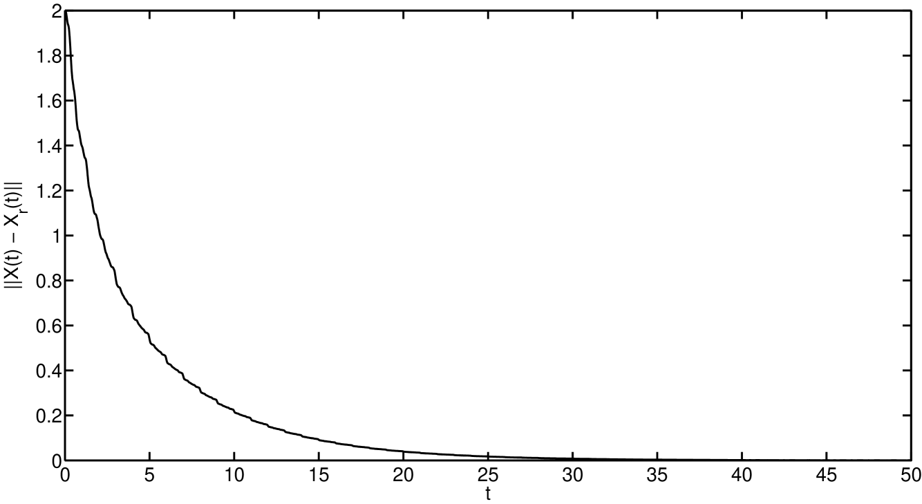
Figure 1: Convergence of the norm of the tracking error to zero.

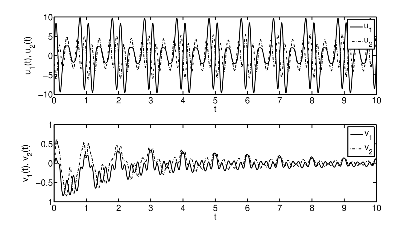
Figure 2: Controls $u_{1},u_{2}$ and “feedbacks” $v_{1},v_{2}$ on the interval $[0,10]$.

IV CONCLUDING REMARKS

In the solution here presented for the periodic motion planning problem, the only needed assumption is that system (1) is regular, which requires that the periodic functions $u_{k}^{T}$ satisfying (3) are explicitly known. Nevertheless, this will hardly be the case in general. For this reason, currently under investigation is the explicit determination of $u_{k}^{r}$ in (2) in a manner that Theorem 1 still holds under assumptions other than the regularity of system (1).

V ACKNOWLEDGMENTS

The authors would like to thank Jean-Michel Coron and Mazyar Mirrahimi for valuable discussions and suggestions.

Appendix A Proof of Lemma 3

In order to prove Theorem 1, we need first a few intermediate definitions and results. For simplicity, we consider throughout this section that $q=(t_{0},W_{t_{0}})\in\mathbb{R}\times\mbox{SU}(n)$ is fixed and that $W_{q}$: $\mathbb{R}\rightarrow\mbox{SU}(n)$ denotes the solution of the auxiliar system (8)–(9) with initial condition $W_{q}(t_{0})=W_{t_{0}}$.

Definition 2

[11] A point $\overline{W}\in M^{n}$ is called a limit point of $W_{q}$ if there exists a real sequence $\{t_{m}\}$ such that $\lim_{m\rightarrow\infty}t_{m}=\infty$ and $\lim_{m\rightarrow\infty}W_{q}(t_{m})=\overline{W}$. The set of all limit points of $W_{q}$ is called the limit set of $W_{q}$ and is denoted by $\Omega(W_{q})$.

Remark 3

Since $\mbox{SU}(n)$ is a compact subset of $M^{n}$, it is clear that $\Omega(W_{q})$ is a non-empty subset of $\mbox{SU}(n)$.

Proposition 1

[11] $\lim_{t\rightarrow\infty}d(W_{q}(t),\Omega(W_{q}))=0$.

The next $2$ lemmas are essential in the proof of the important convergence result of Theorem 3 given below, which was inspired in the periodic version of LaSalle’s invariance principle presented in [11] and in the ad-condition stabilization method of [6].

Lemma 1

Let $W$: $\mathbb{R}\rightarrow M^{n}$ be a continuously differentiable mapping such that $\lim_{t\rightarrow\infty}\dot{W}(t)=0$. Suppose that $\{t_{m}\}$ is a real sequence such that $\lim_{m\rightarrow\infty}t_{m}=\infty$ and $\lim_{m\rightarrow\infty}W(t_{m})=\overline{W}$. Then, for every $\epsilon\in\mathbb{R}$, we have that $\lim_{m\rightarrow\infty}W(t_{m}+\epsilon)=\overline{W}$.

Proof:

Let $\epsilon\geq 0$ and $m\in\mathbb{N}$. We have that $W(t_{m}+\epsilon)-W(t_{m})=\int_{t_{m}}^{t_{m}+\epsilon}\dot{W}(t)\,dt.$ Thus, the inequality $\|W(t_{m}+\epsilon)-W(t_{m})\|\leq|\epsilon|\sup_{t\in[t_{m},t_{m}+\epsilon]}\|\dot{W}(t)\|$ holds. The assumptions then imply that $\lim_{m\rightarrow\infty}W(t_{m}+\epsilon)=\overline{W}$. For $\epsilon<0$, we can proceed in an analogous manner. ∎

Lemma 2

Consider that $\overline{W}\in\Omega(W_{q})$, $j\in\mathbb{N}$ and let $1\leq k\leq m$. Assume that $\lim_{t\rightarrow\infty}\dot{W_{q}}(t)=0$ and that $\lim_{t\rightarrow\infty}\mathrm{V}(W_{q}(t)X^{{\dagger}}_{r}(t)B^{j}_{k}(t)X_{\infty})=0$, where $B^{j}_{k}$ is as in (3). Then, $\mathrm{V}(\overline{W}X^{{\dagger}}_{\infty}B^{j}_{k}(0)X_{\infty})=0$.

Proof:

Let $\overline{W}\in\Omega(W_{q})$. By definition, there exists a real sequence $\{t_{m}\}$ such that $\lim_{m\rightarrow\infty}t_{m}=\infty$ and $\lim_{m\rightarrow\infty}W_{q}(t_{m})=\overline{W}$. Now, for each $m\in\mathbb{N}$, there exists $\ell_{m}\in\mathbb{Z}$ such that $s_{m}=t_{m}-\ell_{m}T\in[0,T)$, where $T>0$ is the period of $X_{r}$ and of $B^{j}_{k}$ (see Remark 1). Since $[0,T]$ is compact, there exists a subsequence $\{s_{m_{i}}\}$ in which $\lim_{i\rightarrow\infty}s_{m_{i}}=\theta\in[0,T]$. Let $\{t_{m_{i}}\}$ be the corresponding subsequence of $\{t_{m}\}$. Define the sequences $\{t^{*}_{m_{i}}\}$ and $\{s^{*}_{m_{i}}\}$ as $t^{*}_{m_{i}}=t_{m_{i}}-\theta$ and $s^{*}_{m_{i}}=s_{m_{i}}-\theta$, respectively. We have that $\lim_{t\rightarrow\infty}\dot{W}_{q}(t)=0$ as well as $\lim_{t\rightarrow\infty}\mathrm{V}(W_{q}(t)X^{{\dagger}}_{r}(t)B^{j}_{k}(t)X_{\infty})=0$ (assumptions). Therefore, by definition, $\lim_{i\rightarrow\infty}s^{*}_{m_{i}}=0$, and Lemma 1 gives that $\lim_{i\rightarrow\infty}W_{q}(t^{*}_{m_{i}})=\lim_{i\rightarrow\infty}W_{q}(t_{m_{i}}-\theta)=\overline{W}$. Hence, the continuity and periodicity of $X_{r}$ and of $B^{j}_{k}$ imply that $\lim_{i\rightarrow\infty}\mathrm{V}(W_{q}(t^{*}_{m_{i}})X^{{\dagger}}_{r}(t^{*}_{m_{i}})B^{j}_{k}(t^{*}_{m_{i}})X_{\infty})=\lim_{i\rightarrow\infty}\mathrm{V}(W_{q}(t^{*}_{m_{i}})X^{{\dagger}}_{r}(s^{*}_{m_{i}})B^{j}_{k}(s^{*}_{m_{i}})X_{\infty})=\mathrm{V}(\overline{W}X^{{\dagger}}_{\infty}B^{j}_{k}(0)X_{\infty})=0$. ∎

Theorem 3

Consider the subset $E=\{W\in\mbox{SU}(n):\mathrm{V}(WX^{{\dagger}}_{\infty}B^{j}_{k}(0)X_{\infty})=0$, for all $j\in\mathbb{N},1\leq k\leq m\}$, where $B^{j}_{k}$ is as in (3). Then, $\lim_{t\rightarrow\infty}d(W_{q}(t),E)=0$ and $E$ is non-empty.

Proof:

Due to Proposition 1, it suffices to prove that the non-empty limit set $\Omega(W_{q})$ of the solution $W_{q}$ is contained in the set $E$. We remark that since $\mathrm{V}$: $M^{n}\rightarrow\mathbb{R}$ is a continuous linear function, there exists $c>0$ such that $|\mathrm{V}(X)|\leq c\|X\|$, for all $X\in M^{n}$. Furthermore, it follows from (2), (8)–(9), Remark 1 and the compactness of $\mbox{SU}(n)$ that each of the mappings $X_{r}$, $X^{\dagger}_{r}$, $W_{q}$, $B^{j}_{k}$, $\dot{X}_{r}$, $\dot{X}^{\dagger}_{r}$, $\dot{W}_{q}$, $\dot{B}^{j}_{k}$ is bounded, for every $j\in\mathbb{N}$, $1\leq k\leq m$.

Consider the functions $\alpha$: $\mathbb{R}\rightarrow\mathbb{R}$, $b^{j}_{k}$: $\mathbb{R}\times M^{n}\rightarrow\mathbb{R}$, $\beta^{j}_{k}$: $\mathbb{R}\rightarrow\mathbb{R}$ defined respectively as

$$\begin{array}[]{ll}\alpha(t)=\mathrm{V}(W_{q}(t)),&\mbox{for all }t\in\mathbb{R},\\ b^{j}_{k}(t,W)=\mathrm{V}(WX^{{\dagger}}_{r}(t)B^{j}_{k}(t)X_{\infty}),&(t,W)\in\mathbb{R}\times M^{n},\\ \beta^{j}_{k}(t)=b^{j}_{k}(t,W_{q}(t)),&\mbox{for all }t\in\mathbb{R},\end{array}$$

for $j\in\mathbb{N}$, $1\leq k\leq m$. We will prove by induction that

$$\lim_{t\rightarrow\infty}\beta^{j}_{k}(t)=\lim_{t\rightarrow\infty}\mathrm{V}(W_{q}(t)X^{{\dagger}}_{r}(t)B^{j}_{k}(t)X_{\infty})=0,$$ (16)

for $j\in\mathbb{N}$, $1\leq k\leq m$. From (8)–(9) and the definition of $b^{0}_{k}$, we have that $\dot{\mathrm{V}}(t,W)=\sum_{k=1}^{m}f_{k}^{2}b^{0}_{k}(t,W)^{2}\geq 0$ and $\ddot{\mathrm{V}}(t,W)=2\sum_{k=1}^{m}f_{k}^{2}\dot{b}^{0}_{k}(t,W)b^{0}_{k}(t,W)$, where $\dot{b}^{0}_{k}(t,W)=\mathrm{V}(WX^{{\dagger}}_{r}(t)\sum_{\ell=1}^{m}f^{2}_{\ell}b^{0}_{\ell}(t,W)H_{\ell}B^{0}_{k}(t)X_{\infty})+b^{1}_{k}(t,W)$ and $f_{1},\dots,f_{m}\in\mathbb{R}$ are non-zero, for $(t,W)\in\mathbb{R}\times M^{n}$. Since $\dot{\mathrm{V}}$ is a non-negative function, we conclude that $\alpha$ is a non-decreasing function bounded from above such that $\ddot{\alpha}$ is bounded. Hence, $\lim_{t\rightarrow\infty}\alpha(t)$ exists and is finite. This relation along with Barbalat’s Lemma (see e.g. [10]) give that $\lim_{t\rightarrow\infty}\dot{\alpha}(t)=\sum_{k=1}^{m}f_{k}^{2}b^{0}_{k}(t,W_{q}(t))^{2}=0$. Thus, $\lim_{t\rightarrow\infty}\beta^{0}_{k}(t)=\lim_{t\rightarrow\infty}\mathrm{V}(W_{q}(t)X^{{\dagger}}_{r}(t)B^{0}_{k}(t)X_{\infty})=0$, for each $1\leq k\leq m$, from which (8)–(9) imply that

$$\lim_{t\rightarrow\infty}\dot{W}_{q}(t)=0.$$ (17)

Now, consider the induction hypothesis

$$\lim_{t\rightarrow\infty}\beta^{j}_{k}(t)=\lim_{t\rightarrow\infty}\mathrm{V}(W_{q}(t)X^{{\dagger}}_{r}(t)B^{j}_{k}(t)X_{\infty})=0,$$ (18)

for some $j\in\mathbb{N}$ and all $1\leq k\leq m$. We have that $\dot{b}^{j}_{k}(t,W)=\mathrm{V}(WX^{{\dagger}}_{r}(t)\sum_{\ell=1}^{m}f^{2}_{\ell}b^{0}_{\ell}(t,W)H_{\ell}B^{j}_{k}(t)X_{\infty})+b^{j+1}_{k}(t,W)$, for all $1\leq k\leq m$, $(t,W)\in\mathbb{R}\times M^{n}$. Straightforward computations show that $\ddot{\beta}^{j}_{k}$ is bounded because $\ddot{\beta}^{j}_{k}(t)=\ddot{b}^{j}_{k}(t,W_{q}(t))$, for all $1\leq k\leq m$, $t\in\mathbb{R}$. Hence, (18) and Barbalat’s Lemma imply that $\lim_{t\rightarrow\infty}\beta^{j+1}_{k}(t)=\lim_{t\rightarrow\infty}\mathrm{V}(W_{q}(t)X^{{\dagger}}_{r}(t)B^{j+1}_{k}(t)X_{\infty})=0$, for $1\leq k\leq m$. We have thus proved that (16) is true. At this moment, it is simple to prove that $\Omega(W_{q})\subset E$. Indeed, assume that $\overline{W}\in\Omega(W_{q})\subset\mbox{SU}(n)$. Then, (16), (17) and Lemma 2 imply that $\mathrm{V}(\overline{W}X^{{\dagger}}_{\infty}B^{j}_{k}(0)X_{\infty})=0$, for each $j\in\mathbb{N}$, $1\leq k\leq m$. ∎

Lemma 3

Consider the subset $F=\{W\in\mbox{SU}(n):V(W)=\sum_{i=1}^{n}\Re(\lambda_{i}),\mbox{ for some }\lambda_{i}\in\mathbb{C}\mbox{ such that }|\lambda_{i}|=1,\prod_{i=1}^{n}\lambda_{i}=1,\Im(\lambda_{1})=\dots=\Im(\lambda_{n})\}$. Then, $I\in F$ and $\lim_{t\rightarrow\infty}d(W_{q}(t),F)=0$.

Proof:

According to Theorem 3, it suffices to show the inclusion $E\subset F$. Let $W\in E\subset\mbox{SU}(n)$. It is a well-known result in linear algebra that $W\in\mbox{SU}(n)$ can be decomposed as $W=M\mbox{diag}(\lambda_{1},\dots,\lambda_{n})M^{\dagger}$, where $M$ is unitary, $\lambda_{1},\dots,\lambda_{n}\in\mathbb{C}$, $|\lambda_{i}|=1$ and $\prod_{i=1}^{n}\lambda_{i}=1$. Thus, $V(W)=\sum_{i=1}^{n}\Re(\lambda_{i})$ and $\mathrm{V}(WX^{{\dagger}}_{\infty}B^{j}_{k}(0)X_{\infty})=\mathrm{V}(\mbox{diag}(\lambda_{1},\dots,\lambda_{n})(X_{\infty}M)^{\dagger}B^{j}_{k}(0)(X_{\infty}M))=0$, for each $1\leq k\leq m$, $j\in\mathbb{N}$. Since $X_{\infty}M$ is unitary, it is clear that $N$: $\mathfrak{su}(n)\rightarrow\mathfrak{su}(n)$ defined by $N(Y)=(X_{\infty}M)^{\dagger}Y(X_{\infty}M)$, for every $Y\in\mathfrak{su}(n)$, is a linear surjective isomorphism. Now, by assumption, system (1) is regular and (3) is satisfied. Hence, $\mathrm{V}(\mbox{diag}(\lambda_{1},\dots,\lambda_{n})X)=0$, for every $X\in\mathfrak{su}(n)$, and thus $\mathrm{V}(\mbox{diag}(\lambda_{1},\dots,\lambda_{n})D_{\ell})=0$, for each $1\leq\ell\leq n$, where $D_{1}=\mbox{diag}(\imath,-\imath,0,\dots,0)$, $D_{2}=\mbox{diag}(0,\imath,-\imath,0,\dots,0),\dots,D_{n-1}=\mbox{diag}(0,\dots,\imath,-\imath)$ and $D_{n}=\mbox{diag}(\imath,0,\dots,0,-\imath)$ are the canonical diagonal matrices of $\mathfrak{su}(n)$. From the diagonal structure of $D_{1},\dots,D_{n}$, we conclude that $\lambda_{1},\dots,\lambda_{n}$ must satisfy $\Im(\lambda_{1})=\dots=\Im(\lambda_{n})$. This implies that $W\in F$ and therefore $E\subset F$. ∎

The proof of Theorem 1 is given below.

Proof:

It is clear that $n=\max{(G)}$ because $I\in F$. We will first show that $G$ is finite. Let $x\in G$. Then, there exist $\lambda_{1},\dots,\lambda_{n}\in\mathbb{C}$ such that $x=\sum_{j=1}^{n}\Re(\lambda_{j})$ with (i) $\prod_{j=1}^{n}\lambda_{j}$, (ii) $|\lambda_{j}|=1$ and (iii) $\Im(\lambda_{1})=\dots=\Im(\lambda_{n})$. Property (ii) implies that $\lambda_{j}=e^{\imath\theta_{j}}$, for some $\theta_{j}\in\mathbb{R}$, and it follows from (iii) that $\lambda_{j}=\lambda_{1}=e^{\imath\theta_{1}}$ or $\lambda_{j}=e^{\imath(\pi-\theta_{1})}$, for each $1\leq j\leq n$. Let $n_{1}$ be the number of $j\in\{1,\dots,n\}$ such that $\lambda_{j}=\lambda_{1}$ and define $n_{2}=n-n_{1}$. Therefore, $x=n_{1}\cos(\theta_{1})+n_{2}\cos(\pi-\theta_{1})=(n_{1}-n_{2})\cos(\theta_{1})$ with $n_{1},(n_{2}+1)\in\{1,\dots,n\}$ and $n_{1}+n_{2}=n$. If $n_{1}=n_{2}$, then $x=0$. Thus, assume that $n_{1}\neq n_{2}$. From property (i) we obtain that $e^{\imath n_{1}\theta_{1}}e^{\imath n_{2}(\pi-\theta_{1})}=1$. Hence, there exists $k\in\mathbb{Z}$ such that $n_{1}\theta_{1}+n_{2}(\pi-\theta_{1})=2k\pi$. This relation implies that $\theta_{1}=(2k-n_{2})\pi/(n-2n_{2})$. Note that $n_{1},n_{2},k$ depend on $x\in G$ and that $n_{2}$, $n_{1}-n_{2}$ can only assume a finite number of values. If we show that $\theta_{1}$ can only assume a finite number of values, we will have shown that the same holds for $x\in G$, which implies that $G$ is finite. It is clear that the function $\eta$: $\mathbb{Z}\rightarrow\mathbb{R}$ defined as $\eta(\ell)=\cos((2\ell-n_{2})\pi/(n-2n_{2}))$, for all $\ell\in\mathbb{Z}$, has period $|n-2n_{2}|>0$. Thus, the values assumed by $\theta_{1}$ must be finite in number.

Now, the convergence result will be shown. Recall that, for all $X\in\mbox{SU}(n)$, we have that $-n\leq V(X)\leq n$ and that $V(X)=n$ if and only if $X=I$. Let $\delta=\max(G\setminus\{n\})$. Since $G$ is finite, we have that

$$\delta<x\leq n\Rightarrow x=n,\hskip 12.0pt\mbox{ for all }x\in G.$$ (19)

Suppose that $V(W_{t_{0}})>\delta$. Since $\mbox{SU}(n)$ is compact and $V$: $M^{n}\rightarrow\mathbb{R}$ is continuous, it follows that $V|\mbox{SU}(n)$ is uniformly continuous. Define the function $\alpha$: $\mathbb{R}\rightarrow\mathbb{R}$ by $\alpha(t)=\mathrm{V}(W_{q}(t))$, for $t\in\mathbb{R}$. Recall that, by construction, we have that $\dot{\mathrm{V}}(t,W)=\sum_{k=1}^{m}a_{k}(t,W)^{2}\geq 0$, for all $(t,W)\in\mathbb{R}\times M^{n}$. Note that $a_{k}$ and $\dot{\mathrm{V}}$ are smooth, for each $1\leq k\leq m$. Since $\dot{\mathrm{V}}$ is a non-negative function, we conclude that $\alpha$ is a smooth non-decreasing function. Therefore, $V(W_{q}(t))\geq V(W_{t_{0}})>\delta$, for all $t\geq t_{0}$. The uniform continuity of $V|\mbox{SU}(n)$ then implies that there exists $\mu>0$ such that

$$\|X-W_{q}(t)\|<\mu\Rightarrow V(X)>\delta,\hskip 12.0pt\mbox{ for }t\geq t_{0},\;X\in\mbox{SU}(n)$$ (20)

(indeed, choose $\epsilon=V(W_{t_{0}})-\delta>0$). The convergence result of Lemma 3 means that

$$\forall\epsilon>0\;\exists\overline{T}\in\mathbb{R}\;\forall t\geq\overline{T}\;\exists\alpha(t)\in F\mbox{ s.t. }\|\alpha(t)-W_{q}(t)\|<\epsilon.$$

Let $\epsilon>0$ and define $\overline{\epsilon}=\min(\epsilon,\mu)$. Thus,

$$\forall t\geq\overline{T}\;\exists\alpha(t)\in F\mbox{ s.t. }\|\alpha(t)-W_{q}(t)\|<\overline{\epsilon}\leq\mu,$$

for some $\overline{T}\in\mathbb{R}$. Define $\widetilde{T}=\max(\overline{T},t_{0})$ and let $t\geq\widetilde{T}$. Since $\alpha(t)\in F\subset\mbox{SU}(n)$ and $V(F)\subset G$, (20) gives that $\delta<V(\alpha(t))\in G$. However, $\delta<V(\alpha(t))\leq n$. Therefore, from (19), we obtain that $V(\alpha(t))=n$, which implies that $\alpha(t)=I$. We have thus shown that $\lim_{t\rightarrow\infty}W_{q}(t)=I$. ∎

References

- [1] F. Albertini and D. D’Alessandro. Notions of controllability for bilinear multilevel quantum systems. IEEE Trans. Automat. Control, 48(8):1399–1403, 2003.
- [2] J.-M. Coron. Linearized control systems and applications to smooth stabilization. SIAM J. Control Optim., 32(2):358–386, 1994.
- [3] J.-M. Coron. Control and Nonlinearity. American Mathematical Society, 2007.
- [4] D. D’Alessandro. Introduction to Quantum Control and Dynamics. Chapman & Hall/CRC, Boca Raton, 2008.
- [5] S. Haroche and J-M. Raimond. Exploring the Quantum: Atoms, Cavities and Photons. Oxford University Press, Oxford, 2006.
- [6] V. Jurdjevic and J. P. Quinn. Controllability and stability. J. Diff. Equations, 28:381–389, 1978.
- [7] M. A. Nielsen and I. L. Chuang. Quantum Computation and Quantum Information. Cambridge Universisty Press, Cambridge, 2000.
- [8] P. S. Pereira da Silva and P. Rouchon. Flatness-based control of a single qubit gate. IEEE Trans. Automat. Control, 53(3):775–779, 2008.
- [9] P. Rouchon. Quantum systems and control. ARIMA, 9:325–357, 2008.
- [10] J.-J. E. Slotine and W. Li. Applied Nonlinear Control. Prentice Hall, New Jersey, 1991.
- [11] M. Vidyasagar. Nonlinear Systems Analysis. Prentice Hall, New Jersey, 2nd edition, 1993.