${\bm{B}}$-mode CMB Polarization from Patchy Screening during Reionization

Abstract

$B$-modes in CMB polarization from patchy reionization arise from two effects: generation of polarization from scattering of quadrupole moments by reionization bubbles, and fluctuations in the screening of $E$-modes from recombination. The scattering contribution has been studied previously, but the screening contribution has not yet been calculated. We show that on scales smaller than the acoustic scale ($\ell\gtrsim 300$), the B-mode power from screening is larger than the B-mode power from scattering. The ratio approaches a constant $\sim$2.5 below the damping scale ($\ell\gtrsim 2000$). On degree scales relevant for gravitational waves ($\ell\lesssim 100$), screening $B$-modes have a white noise tail and are subdominant to the scattering effect. These results are robust to uncertainties in the modeling of patchy reionization.

I Introduction

In linear theory, the presence of a curl or $B$-mode pattern in the polarization of the CMB is an indication that there are contributions from gravitational waves or vector perturbations that, unlike density perturbations, can impart a sense of handedness to the polarization. Beyond linear theory, it is well known that second order effects such as gravitational lensing can produce $B$-modes from density fluctuations Zaldarriaga and Seljak (1998). In fact, any process that modulates the polarization amplitude, direction, or position on the sky can generate $B$-modes from the intrinsic $E$-modes at recombination (e.g. Hu et al. (2003)).

In this Brief Report, we study one such contribution: the amplitude modulation due to patchy screening of the primary polarization due to inhomogeneous reionization. Whereas the analogous effect of patchy generation of polarization from scattering of the quadrupole anisotropy during reionization has been well-studied in the literature Hu (2000a); Weller (1999); Liu et al. (2001); Santos et al. (2003); Mortonson and Hu (2007); Dore et al. (2007), patchy screening is usually neglected as a small contribution. While negligible at large angles, we show here that the two effects are always comparable in magnitude beyond the damping tail with $\sim 2.5$ times as much power in the screening effect.

II Patchy Screening

II.1 Formalism

Scattering of CMB radiation during reionization out of the line of sight suppresses the primary temperature and polarization anisotropy from recombination as $e^{-\tau}$ where $\tau$ is the Thomson optical depth. If $\tau$ varies across the line of sight this suppression itself introduces anisotropy as

$$T(\widehat{\bf n}) = e^{-\tau(\widehat{\bf n})}T^{({\rm rec})}(\widehat{\bf n})\,,$$

$$(Q\pm iU)(\widehat{\bf n}) = e^{-\tau(\widehat{\bf n})}(Q\pm iU)^{({\rm rec})}(\widehat{\bf n})\,,$$ (1)

where $T$ is the temperature fluctuation and $Q$ and $U$ are the polarization Stokes parameters, and we have assumed that the dominant temperature fluctuations from recombination are below the angular scale subtended by the horizon during reionization. These recombination fluctuations can be decomposed in multipole moments in the usual way with the additional assumption that the polarization contains $E$-modes only

$$T^{({\rm rec})}(\widehat{\bf n}) = \sum_{\ell m}T_{\ell m}^{({\rm rec})}Y_{\ell m}(\widehat{\bf n})\,,$$

$$(Q\pm iU)^{(\rm rec)}(\widehat{\bf n}) = -\sum_{\ell m}(E_{\ell m}^{({\rm rec})}\pm iB_{\ell m}^{({\rm rec})})[{}_{\pm 2}Y_{\ell m}(\widehat{\bf n})]$$ (2)

$$= -\sum_{\ell m}E_{\ell m}^{({\rm rec})}[{}_{\pm 2}Y_{\ell m}(\widehat{\bf n})]\,.$$

Decomposing the anisotropic part of the optical depth into multipole moments

$$\tau(\widehat{\bf n}) = \bar{\tau}+\sum_{\ell\geq 1}\sum_{m}\tau_{\ell m}Y_{\ell m}(\widehat{\bf n})\,,$$ (3)

we obtain in the $(\tau(\widehat{\bf n})-\bar{\tau})\ll 1$ limit

$$T_{\ell m}^{({\rm scr})} = -e^{-\bar{\tau}}\sum_{\ell^{\prime}m^{\prime}\ell^{\prime\prime}m^{\prime\prime}}\tau_{\ell^{\prime\prime}m^{\prime\prime}}T_{\ell^{\prime}m^{\prime}}^{({\rm rec})}$$ (7)

$$\times(-1)^{m}\sqrt{2\ell+1}W_{\ell\ell^{\prime}\ell^{\prime\prime}}^{000}\left(\begin{array}[]{ccc}\!\ell\!&\ell^{\prime}\!&\ell^{\prime\prime}\!\\ \!-m\!&m^{\prime}\!&m^{\prime\prime}\!\end{array}\right)\,,$$

$$E_{\ell m}^{(\rm scr)} = -e^{-\bar{\tau}}\sum_{\ell^{\prime}m^{\prime}\ell^{\prime\prime}m^{\prime\prime}}\tau_{\ell^{\prime\prime}m^{\prime\prime}}E_{\ell^{\prime}m^{\prime}}^{(\rm rec)}e_{\ell\ell^{\prime}\ell^{\prime\prime}}$$ (10)

$$\times(-1)^{m}\sqrt{2\ell+1}W_{\ell\ell^{\prime}\ell^{\prime\prime}}^{220}\left(\begin{array}[]{ccc}\!\ell\!&\ell^{\prime}\!&\ell^{\prime\prime}\!\\ \!-m\!&m^{\prime}\!&m^{\prime\prime}\!\end{array}\right)\,,$$

$$iB_{\ell m}^{(\rm scr)} = -e^{-\bar{\tau}}\sum_{\ell^{\prime}m^{\prime}\ell^{\prime\prime}m^{\prime\prime}}\tau_{\ell^{\prime\prime}m^{\prime\prime}}E_{\ell^{\prime}m^{\prime}}^{(\rm rec)}o_{\ell\ell^{\prime}\ell^{\prime\prime}}$$ (13)

$$\times(-1)^{m}\sqrt{2\ell+1}W_{\ell\ell^{\prime}\ell^{\prime\prime}}^{220}\left(\begin{array}[]{ccc}\!\ell\!&\ell^{\prime}\!&\ell^{\prime\prime}\!\\ \!-m\!&m^{\prime}\!&m^{\prime\prime}\!\end{array}\right)\,,$$

where $e_{\ell\ell^{\prime}\ell^{\prime\prime}}=[1+(-1)^{\ell+\ell^{\prime}+\ell^{\prime\prime}}]/2$ and $o_{\ell\ell^{\prime}\ell^{\prime\prime}}=[1-(-1)^{\ell+\ell^{\prime}+\ell^{\prime\prime}}]/2$ picks out even and odd triplets and

$$W_{\ell\ell^{\prime}\ell^{\prime\prime}}^{ss^{\prime}s^{\prime\prime}}=\sqrt{{(2\ell^{\prime}+1)(2\ell^{\prime\prime}+1)\over 4\pi}}\left(\begin{array}[]{ccc}\!\ell\!&\ell^{\prime}\!&\ell"\!\\ \!-s\!&s^{\prime}\!&s^{\prime\prime}\!\end{array}\right)\,.$$ (16)

Here we have given the contribution to the anisotropy from the $\ell>0$ terms in $e^{-\tau}$:

$$X_{\ell m}^{\rm(scr)}=X_{\ell m}-\langle e^{-\tau}\rangle X_{\ell m}^{\rm(rec)}\,,$$ (17)

where $X\in\{T,E,B\}$. The additional power spectra contributions

$$\langle X_{\ell m}^{*}Y_{\ell^{\prime}m^{\prime}}\rangle=\delta_{\ell\ell^{\prime}}\delta_{mm^{\prime}}C_{\ell}^{XY}\,,$$ (18)

become Hu et al. (2003)

$$C_{\ell}^{TT({\rm scr})} = e^{-2\bar{\tau}}\sum_{\ell^{\prime}\ell^{\prime\prime}}C_{\ell^{\prime\prime}}^{\tau\tau}C_{\ell^{\prime}}^{TT({\rm rec})}(W_{\ell\ell^{\prime}\ell^{\prime\prime}}^{000})^{2}\,,$$

$$C_{\ell}^{TE({\rm scr})} = e^{-2\bar{\tau}}\sum_{\ell^{\prime}\ell^{\prime\prime}}C_{\ell^{\prime\prime}}^{\tau\tau}C_{\ell^{\prime}}^{TE({\rm rec})}(W_{\ell\ell^{\prime}\ell^{\prime\prime}}^{000}W_{\ell\ell^{\prime}\ell^{\prime\prime}}^{220})\,,$$

$$C_{\ell}^{EE({\rm scr})} = e^{-2\bar{\tau}}\sum_{\ell^{\prime}\ell^{\prime\prime}}C_{\ell^{\prime\prime}}^{\tau\tau}C_{\ell^{\prime}}^{EE({\rm rec})}e_{\ell\ell^{\prime}\ell^{\prime\prime}}(W_{\ell\ell^{\prime}\ell^{\prime\prime}}^{220})^{2}\,,$$

$$C_{\ell}^{BB({\rm scr})} = e^{-2\bar{\tau}}\sum_{\ell^{\prime}\ell^{\prime\prime}}C_{\ell^{\prime\prime}}^{\tau\tau}C_{\ell^{\prime}}^{EE({\rm rec})}o_{\ell\ell^{\prime}\ell^{\prime\prime}}(W_{\ell\ell^{\prime}\ell^{\prime\prime}}^{220})^{2}\,.$$ (19)

We evaluate the recombination power spectra by setting $\tau=0$. These sums can be efficiently evaluated in position space as shown in the Appendix.

Note that in the decomposition defined in Eqn. (17), the isotropic screening term gains a contribution from the rms fluctuations in $\tau$

$$\langle e^{-\tau}\rangle^{2}\langle X_{\ell m}^{\rm(rec)*}Y_{\ell^{\prime}m^{\prime}}^{\rm(rec)}\rangle\approx\delta_{\ell\ell^{\prime}}\delta_{mm^{\prime}}e^{-2\bar{\tau}}(1+\tau_{\rm rms}^{2})C_{\ell}^{XY({\rm rec})}$$

where

$$\tau_{\rm rms}^{2}=\sum_{\ell\geq 1}{2\ell+1\over 4\pi}C_{\ell}^{\tau\tau}\,.$$ (20)

This term is ordinarily not included in the standard calculation but is a correction that is second order in $(\tau(\widehat{\bf n})-\bar{\tau})$.

II.2 ${\bm{B}}$-Mode Scaling

We now focus on the $B$-mode generation from screening and its relationship to other secondary effects. To extract the large and small angle scaling behavior of the $B$-modes it is useful to take the flat-sky approximation where Fourier moments replace harmonic coefficients

$$(Q\pm iU)(\widehat{\bf n})=\int{d^{2}{{\bm{\ell}}}\over(2\pi)^{2}}[E({{\bm{\ell}}})\pm iB({{\bm{\ell}}})]e^{\pm 2i\phi_{\bm{\ell}}}e^{i{{\bm{\ell}}}\cdot{\widehat{\bf n}}}\,,$$ (21)

where $\phi_{{\bm{\ell}}}$ denotes the angle between ${{\bm{\ell}}}$ and the axis on which $Q$ is defined. The power spectrum

$$\langle B^{*}({{\bm{\ell}}})B({{\bm{\ell}}}^{\prime})\rangle=(2\pi)^{2}\delta({{\bm{\ell}}}-{{\bm{\ell}}}^{\prime})C_{\ell}^{BB}\,,$$ (22)

then becomes for the screening modes

$$C^{BB({\rm scr})}_{\ell}=e^{-2\bar{\tau}}\int{d^{2}{{{\bm{\ell}}}^{\prime}}\over(2\pi)^{2}}C^{EE({\rm rec})}_{{\ell}^{\prime}}C^{\tau\tau}_{|{{\bm{\ell}}}-{{\bm{\ell}}}^{\prime}|}\sin^{2}{(2\phi_{{{\bm{\ell}}^{\prime}}})}\,,$$ (23)

where we have set $\phi_{{\bm{\ell}}}=0$ for convenience.

The $B$-mode power spectrum therefore represents a convolution of recombination and $\tau$ power spectra. Its main properties are defined by the well-determined shape of the primary $E$-mode power spectrum. In particular, the primary $E$-modes have little power above the acoustic scale $\ell<\ell_{A}\approx 300$ and below the damping scale $\ell>\ell_{D}\approx 2000$. In these two limits, the screening $B$-modes take on a particularly simple form. For $\ell\ll\ell_{A}$,

$$C^{BB({\rm scr})}_{\ell}\approx{e^{-2\bar{\tau}}\over 2}\int{d^{2}{{{\bm{\ell}}}^{\prime}}\over(2\pi)^{2}}C^{EE({\rm rec})}_{{\ell}^{\prime}}C^{\tau\tau}_{{\ell}^{\prime}}={\rm const.}$$ (24)

is white noise in form. Note that this property is independent of the amount of low $\ell$ power in $C_{\ell}^{\tau\tau}$. Only optical depth fluctuations on scales comparable to $\ell_{A}$ can modulate the polarization into large angle $B$-modes.

For $\ell\gg\ell_{D}$, the $B$-modes reflect the shape of the $\tau$ power spectrum

$$C^{BB({\rm scr})}_{\ell}\approx{1\over 2}E_{\rm rms}^{2}{C^{\tau\tau}_{\ell}}e^{-2\bar{\tau}}$$ (25)

with an amplitude that is determined by the total power in the primary $E$-modes

$$E_{\rm rms}^{2}=\int{d^{2}{{\bm{\ell}}}\over(2\pi)^{2}}C^{EE({\rm rec})}_{{\ell}}\approx\sum_{\ell}{2\ell+1\over 4\pi}C^{EE({\rm rec})}_{{\ell}}\,.$$ (26)

Under the damping tail, the primary $E$-modes are much smoother than $\tau$ fluctuations and so $E_{\rm rms}$ simply represents the typical level of $E$-mode that is modulated into small scale $B$-mode polarization by $\tau$.

It is useful to compare these scalings with those of the two other well-known sources of secondary $B$-modes: gravitational lensing and patchy scattering of quadrupole anisotropy at reionization. Lensing obeys a similar form with deflection angles playing the role of $\tau$ and polarization gradients playing the role of $E$. In particular, it has a white noise form for $\ell\ll\ell_{A}$ and follows the deflection power spectrum for $\ell\gg\ell_{D}$ with an amplitude set by the total gradient power in the primary polarization Zaldarriaga and Seljak (1998); Hu (2000b).

For patchy scattering of the quadrupole fluctuations during reionization Hu (2000a)

$$C^{BB({\rm sca})}_{\ell}\approx{3\over 100}{C^{\tau\tau}_{\ell}}Q_{\rm rms}^{2}e^{-2\tau_{\rm eff}}$$ (27)

for scales much smaller than the reionization bump $\ell\gg\ell_{R}\approx 20$. Here $Q_{\rm rms}$ is the rms quadrupole at reionization and $\tau_{\rm eff}$ is the typical optical depth between $z=0$ and the scatterers, so that $\tau_{\rm eff}\lesssim\bar{\tau}$. The crucial difference between this effect and the patchy screening effect is that the quadrupole is coherent on large angles $\ell_{R}\ll\ell_{A}$ and so the $B$-modes are in the small scale limit for all relevant scales.

In particular for $\ell\gg\ell_{D}$,

$${C_{\ell}^{BB({\rm scr})}\over C_{\ell}^{BB({\rm sca})}}\approx{50\over 3}{E_{\rm rms}^{2}\over Q_{\rm rms}^{2}}e^{2(\tau_{\rm eff}-\bar{\tau})}\,.$$ (28)

For the WMAP5 cosmology Komatsu et al. (2009), $\Omega_{b}h^{2}=0.02265$, $\Omega_{m}h^{2}=0.137$, $h=0.701$, $\Omega_{\Lambda}=0.721$, $\bar{\tau}=0.084$, $A_{S}=2.16\times 10^{-9}$, $n_{s}=0.96$, the rms fluctuations are $E_{\rm rms}=6.9\mu$K and $Q_{\rm rms}=17.9\mu$K and so the ratio of power approaches a factor of $\sim 2.5$. Independently of the form of $C_{\ell}^{\tau\tau}$, the screening $B$-modes dominate the scattering ones on scales near the damping tail and below.

Conversely, independently of the power in $C_{\ell}^{\tau\tau}$ at multipoles $\ell<\ell_{A}$, the screening $B$-modes fall as white noise whereas the scattering ones can continue to rise if there is large-scale power in $\tau$. Therefore only the scattering $B$-modes are relevant as contamination to the gravitational wave signal at $\ell\sim 100$.

We show examples of these behaviors in Fig. 1. We take two representative models, a “fiducial” model in which $C_{\ell}^{\tau\tau}$ has only small scale power contributed by relatively small ionization patches, and a “maximal” model which has substantial power at $\ell\sim 100$ from patches that are substantially larger than those expected in current models of reionization. The large-bubble model maximizes the scattering $B$-mode contamination to the gravitational wave signal Mortonson and Hu (2007).

More precisely, in both models the ionization history $x_{e}(z)$ is the same as the fiducial model in Dvorkin and Smith (2009), where the parameter $\Delta_{y}$ controls the duration of partial ionization. Specifically, our choice of $\Delta_{y}=19$ gives a range of $6\lesssim z\lesssim 14$. The total optical depth to recombination is taken to be $\bar{\tau}=0.084$. During partial reionization, the ionized regions are represented by spherical bubbles with a log-normal distribution Furlanetto et al. (2004); Zahn et al. (2006) with characteristic size given by $\bar{R}$ (in Mpc) and distribution width given by $\sigma_{\ln R}$. We take $\{\bar{R},\sigma_{\ln R}\}=\{5,\ln(2)\}$ in the fiducial model, and $\{\bar{R},\sigma_{\ln R}\}=\{30,\ln(2)\}$ in the large-bubble model. We assume that the bubbles are linearly biased tracers of the large-scale matter density field, with bias $b=6$ using the construction of Ref. Wang and Hu (2006). Note that rms fluctuations in $\tau$ for the small and large-bubble models are $\tau_{\rm rms}=0.007$ and $\tau_{\rm rms}=0.017$ and so both satisfy the condition that $\tau_{\rm rms}\ll\bar{\tau}$.

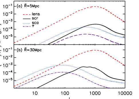
Figure 1: $B$-mode power spectra. Three different contributions are being plotted: lensed $B$-modes, patchy $B$-modes from Thomson scattering, and patchy $B$-modes from screening. The model is the WMAP5 cosmology with (a) the fiducial reionization model of $\{\bar{\tau},\Delta_{y},b,\bar{R},\sigma_{\ln R}\}=\{0.084,19.0,6.0,5\mbox{ Mpc},\ln(2)\}$, and (b) a maximal model with the same parameters except $\bar{R}=30$ Mpc. For reference the $\tau$ power spectrum in dimensionless units is also plotted.

For reference, the small scale limits to the other power spectra for patchy screening can be obtained by replacing $E_{\rm rms}^{2}/2$ with $T_{\rm rms}^{2}$ for temperature in Eqn. (25) where

$$T_{\rm rms}^{2} \approx \sum_{\ell}{2\ell+1\over 4\pi}C^{TT({\rm rec})}_{{\ell}}\,,$$ (29)

whereas the $E$ polarization and $B$ polarization power are equal. The $TE$ cross power spectrum and correlation coefficient is zero in this limit.

III Discussion

Whereas the patchiness of reionization itself remains theoretically uncertain and observationally unconstrained, its effects on CMB polarization are well defined. In addition to the well-known patchy scattering of the quadrupole moment, the patchy screening of primary polarization produces a $B$-mode.

Independently of the form of the patchiness, this contribution is larger than the scattering effect by a factor of $\sim 2.5$ in power on scales below the damping tail. Conversely, on scales above the acoustic scale, the patchy screening effect always falls as white noise unlike the scattering effect. Consequently screening $B$-modes are relatively more important when considering reionization contributions at arcminute scales but are largely unimportant for the degree scales relevant for gravitational wave studies.

Appendix A Efficient Position-space Forms

The harmonic-space forms for the power spectra given in Eqn. (19) naively require computational cost ${\mathcal{O}}(\ell_{\rm max}^{3})$ to compute the power spectrum for all multipoles $\ell\leq\ell_{\rm max}$. For the calculations in this paper (with $\ell_{\rm max}\approx 10^{4}$), we have found it convenient to use position-space forms which are mathematically equivalent but have reduced computational cost ${\mathcal{O}}(\ell_{\rm max}^{2})$:

$$C_{\ell}^{TT({\rm scr})} = 2\pi\int_{-1}^{1}d(\cos{\theta)}d^{\ell}_{00}(\theta)\psi^{TT}(\theta)\psi^{\tau\tau}(\theta)\,,$$

$$C_{\ell}^{TE({\rm scr})} = 2\pi\int_{-1}^{1}d(\cos\theta)\,d^{\ell}_{0,-2}(\theta)\psi^{TE}(\theta)\psi^{\tau\tau}(\theta)\,,$$

$$C_{\ell}^{EE({\rm scr})} = \pi\int_{-1}^{1}d(\cos{\theta)}\big{[}d^{\ell}_{22}(\theta)\psi^{EE}_{+}(\theta)\psi^{\tau\tau}(\theta)$$

$$\quad-d^{\ell}_{2,-2}(\theta)\psi^{EE}_{-}(\theta)\psi^{\tau\tau}(\theta)\big{]}\,,$$

$$C_{\ell}^{BB({\rm scr})} = \pi\int_{-1}^{1}d(\cos{\theta)}\big{[}d^{\ell}_{22}(\theta)\psi^{EE}_{+}(\theta)\psi^{\tau\tau}(\theta)$$ (30)

$$\quad+d^{\ell}_{2,-2}(\theta)\psi^{EE}_{-}(\theta)\psi^{\tau\tau}(\theta)\big{]}\,,$$

where the correlation functions are defined by:

$$\psi^{\tau\tau}(\theta) = e^{-2\bar{\tau}}\sum_{\ell}\left({2\ell+1\over 4\pi}\right)C_{\ell}^{\tau\tau}d^{\ell}_{00}(\theta)\,,$$

$$\psi^{TT}(\theta) = \sum_{\ell}\left({2\ell+1\over 4\pi}\right)C_{\ell}^{TT({\rm rec})}d^{\ell}_{00}(\theta)\,,$$

$$\psi^{TE}(\theta) = \sum_{\ell}\left(\frac{2\ell+1}{4\pi}\right)C_{\ell}^{TE({\rm rec})}d_{02}^{\ell}(\theta)\,,$$

$$\psi^{EE}_{\pm}(\theta) = \pm\sum_{\ell}\left({2\ell+1\over 4\pi}\right)C_{\ell}^{EE({\rm rec})}d^{\ell}_{2,\pm 2}(\theta),$$ (31)

where $d^{\ell}_{2\pm 2}$, $d^{\ell}_{0\pm 2}$ and $d^{\ell}_{00}$ are reduced Wigner $D$-functions. The integrals in Eqn. (30) can be done exactly, using Gauss-Legendre quadrature with $\lceil(3\ell_{\rm max}+1)/2\rceil$ points.

References

• Zaldarriaga and Seljak (1998) M.Β Zaldarriaga and U.Β Seljak, Phys. Rev. D58, 023003 (1998), eprint astro-ph/9803150.
• Hu etΒ al. (2003) W.Β Hu, M.Β M. Hedman, and M.Β Zaldarriaga, Phys. Rev. D67, 043004 (2003), eprint astro-ph/0210096.
• Hu (2000a) W.Β Hu, Astrophys. J. 529, 12 (2000a), eprint astro-ph/9907103.
• Weller (1999) J.Β Weller, Astrophys. J. 527, L1 (1999), eprint astro-ph/9908033.
• Liu etΒ al. (2001) G.-C. Liu, N.Β Sugiyama, A.Β J. Benson, C.Β G. Lacey, and A.Β Nusser (2001), eprint astro-ph/0101368.
• Santos etΒ al. (2003) M.Β G. Santos, A.Β Cooray, Z.Β Haiman, L.Β Knox, and C.-P. Ma, Astrophys. J. 598, 756 (2003), eprint astro-ph/0305471.
• Mortonson and Hu (2007) M.Β J. Mortonson and W.Β Hu, Astrophys. J. 657, 1 (2007), eprint astro-ph/0607652.
• Dore etΒ al. (2007) O.Β Dore etΒ al., Phys. Rev. D76, 043002 (2007), eprint astro-ph/0701784.
• Hu (2000b) W.Β Hu, Phys. Rev. D62, 043007 (2000b), eprint astro-ph/0001303.
• Komatsu etΒ al. (2009) E.Β Komatsu etΒ al. (WMAP), Astrophys. J. Suppl. 180, 330 (2009), eprint 0803.0547.
• Dvorkin and Smith (2009) C.Β Dvorkin and K.Β M. Smith, Phys. Rev. D79, 043003 (2009), eprint 0812.1566.
• Furlanetto etΒ al. (2004) S.Β Furlanetto, M.Β Zaldarriaga, and L.Β Hernquist, Astrophys. J. 613, 1 (2004), eprint astro-ph/0403697.
• Zahn etΒ al. (2006) O.Β Zahn etΒ al., Astrophys. J. 654, 12 (2006), eprint astro-ph/0604177.
• Wang and Hu (2006) X.Β Wang and W.Β Hu, Astrophys. J. 643, 585 (2006), eprint astro-ph/0511141.