The large system asymptotics of persistent currents in mesoscopic quantum rings

Abstract

We consider a one-dimensional mesoscopic quantum ring filled with spinless electrons and threaded by a magnetic flux, which carries a persistent current at zero temperature. The interplay of Coulomb interactions and a single on-site impurity yields a non-trivial dependence of the persistent current on the size of the ring. We determine numerically the asymptotic power law for systems up to $32\,000$ sites for various impurity strengths and compare with predictions from Bethe Ansatz solutions combined with Bosonization. The numerical results are obtained using an improved functional renormalization group (fRG) method. We apply the density matrix renormalization group (DMRG) and exact diagonalization methods to benchmark the fRG calculations. We use DMRG to study the persistent current at low electron concentrations in order to extend the validity of our results to quasi-continuous systems. We briefly comment on the quality of calculated fRG ground state energies by comparison with exact DMRG data.

I Introduction

Quantization of the magnetic flux was first observed in superconducting cylinders Deaver ; Byers . In normal electronic systems the flux quantum $\phi_{0}=hc/e$ determines the period of the persistent currents, which can be observed in mesoscopic one-dimensional disordered metallic rings Buttiker . Persistent currents in metallic rings are induced only if the circumference of the ring is not larger than the electron phase coherence length and/or the electron’s mean-free path. Such conditions can be easily obtained for sufficiently low temperatures at which inelastic scattering from phonons is suppressed. Normally, this happens at temperatures below 1 K and ring sizes of about 1 $\mu$m. Impurities (disorder) in such metallic rings act as elastic scatterers, and it is not surprising that persistent currents can flow despite the non-zero resistance of the rings.

Interest in persistent current phenomena remains strong both experimentally Levy ; Chandrasekhar ; Mailly ; Reulet ; Jariwala ; Rabaut ; Kleemans ; Bouchiat and theoretically  Landauer ; Cheung ; Abraham ; Bouzerar ; Gogolin ; Kato ; Cohen ; Henkel ; Jaimungal ; Meden ; Enss ; Friedrich ; Soroker ; Heinrichs . The main reason for this is the fact that there still is a discrepancy between experiment and theory. Experiments  Levy ; Jariwala show persistent currents which are two orders of magnitude larger than theoretical predictions for rings filled with non-interacting electrons Cheung ; Altshuler ; Henkel . If electron-electron interactions are included, persistent currents increase for repulsive as well as attractive electron interactions Abraham ; Ambegaokar ; Gogolin , however, the calculated currents were still about five times smaller than the experimental data. Recently, Bary-Soroker et al. Soroker provided an explanation for the magnitude of the persistent currents if magnetic impurities and the attractive interactions are considered.

Considerable theoretical effort has been invested into the question whether the interplay between strong electron-electron interactions, electron density, and disorder strength can explain the large persistent currents observed experimentally. Disorder usually gives rise to elastic scattering and consequently should reduce the persistent current. Bouzerar et al. Bouzerar claim that both electron-electron interactions and disorder decrease the persistent current, whereas the self-consistent Hartree-Fock calculations by Cohen et al. Cohen suggest that the current may be enhanced by a moderate disorder due to screening effects. Other theoretical studies conclude that electron-electron interaction could reduce or enhance the current depending on the type of disorder present in the system Abraham ; Cesare ; Gambetti . Abraham and Berkovits Abraham conjectured that the increase would be rather small and one-dimensional spinless models at half-filling cannot explain the results of single ring experiments.

Among the theoretical methods used to study persistent current phenomena are Hartree-Fock approximations Kato ; Cohen , configuration interaction and quantum Monte Carlo simulations Krcmar ; Nemeth , Bosonization Gogolin , conformal field theory Henkel ; Jaimungal , the functional renormalization group (fRG) Meden , and the density matrix renormalization group (DMRG) Meden ; Cesare ; Gambetti .

In the present paper we study the interplay between electron-electron interactions and a single impurity in a one-dimensional system. For one-dimensional interacting systems, the presence of a single impurity is known to affect their physical properties Luther ; Apel ; Kane1 ; Kane2 . We restrict our investigations to the Luttinger liquid phase which is characterized by a power law decay of correlation functions in a sufficiently large system Haldane . Our aim is to investigate the asymptotic behavior of the persistent current $I$ as a function of the ring length $L$, from which the power law exponent may be obtained $I\propto L^{-\alpha_{\rm B}-1}$. The exponent $\alpha_{\rm B}=K^{-1}-1$ is related to the Luttinger liquid parameter $K$ Haldane ; Kane1 ; Kane2 and depends on the electron-electron interaction, but it does not depend on the impurity strength if $L\to\infty$.

It is known that the asymptotics of the currents is reached for smaller system sizes if sufficiently strong impurities are considered Gogolin ; Matveev ; Glazmann . Nevertheless, it is necessary to investigate relatively large systems in order to reach the asymptotics. We therefore need suitable many-body techniques which enable such calculations. We have chosen the functional renormalization group Polchinski ; Wetterich ; Morris ; Salmhofer1 ; Salmhofer2 , which proved to be a rather useful tool in a previous study Meden . However, for numerical reasons the asymptotic regime could not really be reached in that work. In the present paper we improve the fRG technology such that system sizes up to about 32000 lattice sites can be investigated. In order to benchmark the fRG results we use DMRG calculations White1 ; White2 ; Peschel ; Scholl .

We also study the asymptotic power law decay of the persistent current at low electron concentrations in order to clarify differences between discrete lattice models (investigated in this paper) and continuous systems studied by quantum Monte Carlo and configuration interaction methods Nemeth ; Krcmar . For this reason, we apply DMRG to our model away from half-filling ($n=\frac{1}{2}$), in particular, we study the case of quarter-filling ($n=\frac{1}{4}$) as well as $n=\frac{1}{8}$ and $n=\frac{1}{16}$.

The paper is organized as follows. In Sec. 2 we define the model for our calculations and briefly review the theory of the persistent current. We introduce the fRG method in Sec. 3 and related Appendices. Section 4 is devoted to the DMRG method with a short discussion of its limitations. Results are presented in Sec. 5 gathering the numerical data obtained by fRG, DMRG, and exact diagonalization. We calculate the persistent current and extract the effective exponent $\alpha_{\rm eff}$ related to the power law decrease with respect to the ring size $L$. Finally we show DMRG results for systems with low-filling. The results are summarized in Sec. 6.

II Model for spinless Fermions

We consider a quantum ring of interacting spinless electrons at zero temperature. The ring is pierced by a magnetic flux $\phi$ and contains one single impurity. This system is modelled by the tight-binding Hamiltonian

$${\cal H}=-t\sum\limits_{\ell=1}^{L}\left(c^{\dagger}_{\ell}c_{\ell+1}e^{-i\phi/L}+{\rm h.c.}\right)+U\sum\limits_{\ell=1}^{L}n_{\ell}n_{\ell+1}+V\,n_{1}\,,$$ (1)

written in terms of the electron creation and annihilation operators $c^{\dagger}_{\ell}$ and $c_{\ell}$ as well as the electron density operator $n_{\ell}=c_{\ell}^{\dagger}c_{\ell}$.

The Peierls factor $e^{-i\phi/L}$ with $\phi=2\pi\Phi/\Phi_{0}$ describes the influence of the magnetic field in terms of the magnetic flux $\Phi$ Peierls . The flux quantum $\Phi_{0}=hc/e$ is set to one in the following. The hopping amplitude $t$ between neighboring sites is also set to one in order to define the energy scale. The nearest-neighbor Coulomb interaction is denoted by $U$. An (external) on-site impurity potential with strength $V$ is placed on the lattice site $\ell=1$ along the ring ($\ell=1,2,...,L$). Periodic boundary conditions are imposed by $L+1\equiv 1$.

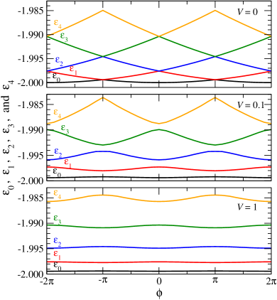
Figure 1: (Color online) The five lowest-laying single-particle energy levels for a non-interacting system as functions of the magnetic flux $\phi$ for a ring of size $L=128$. The three panels correspond to $V=0$, $V=0.1$, and $V=1.0$, respectively.

Without electron-electron interaction ($U=0$) and impurity ($V=0$) the single particle energy levels $\epsilon_{m}$ calculated from the Hamiltonian Eq. (1) depend quadratically on the magnetic flux $\phi$. The persistent current $I_{m}=-v_{m}/L$ at energy level $m$ with the wave vector $k=2\pi\left(\phi+m\right)/L$ is calculated from the electron velocity $v_{m}$,

$$v_{m}(\phi)=2\pi\frac{\partial\epsilon_{m}(\phi)}{\partial k(\phi)}=L\frac{\partial\epsilon_{m}(\phi)}{\partial\phi}\,.$$ (2)

Summation over all occupied energy levels then yields the total persistent current at temperature $T=0$,

$$I(\phi)=-\sum_{m=0}^{m_{\rm max}}\frac{\partial\epsilon_{m}(\phi)}{\partial\phi}\,.$$ (3)

The upper panel in Fig. 1 shows the parabolic energy band structure ($V=0,~{}U=0$). Consequently, the persistent current is proportional to the magnetic flux $\phi$ and inversely proportional to the length $L$ of the ring. For an odd number of electrons in the ring one finds

$$I(\phi)=-\frac{v_{F}}{\pi L}\phi\,,\qquad-\pi\leq\phi<\pi\,,$$ (4)

whereas for an even filling the current is given by

$$I(\phi)=-\frac{v_{F}}{\pi L}\times\left\{\begin{array}[]{ll}\phi+\pi\,,&-\pi\leq\phi<0,\\ \\ \phi-\pi\,,&0\leq\phi<\pi\end{array}\right.$$ (8)

with $v_{\rm F}$ being the Fermi velocity.

An impurity in the ring rounds off the cusps seen in this function as shown in the central and lower panels of Fig. 1 for a weak and an intermediate impurity, respectively. For strong impurities and odd filling, one finds $I\propto-{v_{\rm F}}\sin(\phi)/{\pi L}$ Gogolin . The coupling strength $V$ of an on-site impurity can be related to the physically more relevant transmission coefficient at the Fermi wave vector $k_{\rm F}$

$$T(k_{\rm F})=\frac{4t^{2}}{4t^{2}+V^{2}}\,,$$ (9)

which holds at half-filling in the non-interacting limit SCH98 . With this relation, the strengths of various impurities $V$ used in this paper may be compared.

If the electron-electron interaction $U$ is switched on, the many-body energy levels are shown in Fig. 2 for $U=1$ and various impurity strengths $V$. The persistent currents are obtained from the relation

$$I(\phi)=-\frac{\partial E_{0}(\phi)}{\partial\phi}\,,$$ (10)

where $E_{0}(\phi)$ is the many-body ground-state energy at zero temperature as plotted in Fig. 2. In general the system is a Luttinger liquid. However, at half-filling it is in the Luttinger liquid phase only for $|U|\leq 2$. At $U=2$, the system exhibits a charge-density wave instability, and phase separation characterizes the system for $U<-2$.

In this paper we focus on the Luttinger liquid phase for which Bosonization techniques and additional approximations predict that asymptotically (i.e. for large $L$) the persistent current decays algebraically with increasing system size,

$$I\propto L^{-1-\alpha_{\rm B}}\,.$$ (11)

The exponent $\alpha_{\rm B}$ is a function of the electron-electron interaction (regardless of the impurity strength $V$). Only at half-filling, the exponent $\alpha_{\rm B}$ can be obtained analytically from a Bethe Ansatz solution Haldane ; Meden ; And

$$\alpha_{\rm B}=\frac{2}{\pi}\arccos\left(-\frac{U}{2}\right)-1\,.$$ (12)

Throughout this paper we often consider the case $U=1$ with the corresponding $\alpha_{\rm B}=\frac{1}{3}$. We determine $\alpha_{\rm B}$ from the Hamiltonian Eq. (1) using three different many-body techniques: fRG, DMRG, and exact diagonalization (ED).

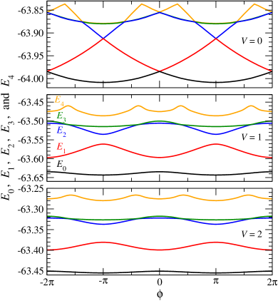
Figure 2: (Color online) The five lowest-laying many-body energy levels obtained by DMRG as a function of the magnetic flux $\phi$ for a ring of size $L=128$ at half-filling and electron-electron interaction $U=1$. Upper panel: $V=0$, center panel: $V=1$, lower panel: $V=2$.

III Functional RG scheme for interacting Fermions

A scheme for one-dimensional Fermionic systems based on the functional renormalization group, has been developed by Meden, Metzner, Schönhammer, and collaborators MED02a based on seminal work by Wetterich Wetterich and Morris Morris . It has been applied to study transport properties of quantum wires MED02a ; MED02b ; AND04 and rings Meden .

The fRG scheme of the present work is similar to the one applied in the references cited above, but uses a somewhat different truncation procedure. Details of our method have been presented recently WEY08 . Here we review the essential steps relevant for a system of spinless interacting Fermions.

The effective average action $\Gamma_{k}$ Wetterich for interacting Fermions evolves according to the fRG equation Wetterich ; BER00

$$\frac{\partial}{\partial k}\Gamma_{k}[\phi^{*},\phi]=-\frac{1}{2}{\rm Tr}\left\{[{\Gamma}_{k}^{(2)}[\phi^{*},\phi]+R_{k}]^{-1}\frac{\partial{R}_{k}}{\partial k}\right\}.$$ (13)

The system of $L$ spinless electrons is described by an $L$-component vector of Grassmann variables $\phi(\tau)=(\phi_{1}(\tau),\ldots,\phi_{L}(\tau))$, which describes the evolution of the interacting Fermionic system in imaginary time $\tau$. The functional derivative of $\Gamma_{k}$ with respect to $\phi^{*}$ and $\phi$ is denoted by $\Gamma_{k}^{(2)}$. The trace in Eq. (13) is to be performed over the Fermionic states $j=1,\ldots,L$. The regulator ${R}_{k}$ is introduced in order to suppress thermal and quantum fluctuations at energy or momentum scales $k$ larger than any physical scale relevant for our problem. With decreasing $k$, the regulator gradually “switches on” such fluctuations until they are fully included at $k=0$, i.e. at $k=0$ the regulator $R_{k}$ vanishes. As a regulator we choose $R_{k}=Ck\theta(k^{2}-\omega^{2})$ with $C$ a large constant and it satisfies all requirements for a useful regulator as discussed in more detail in Ref. WEY08 . It has an additional advantage that the integration over the frequencies $\omega$ can be done analytically.

In order to solve the functional differential equation (13) a particular functional form for $\Gamma_{k}$ in terms of the Grassmann variables $\phi^{*},\phi$ is assumed

$$\Gamma_{k}[\phi^{*},\phi]=\int_{0}^{\beta}{\rm d}\tau\sum_{\alpha=1}^{L}\phi_{\alpha}^{*}(\tau)\frac{\partial}{\partial\tau}\phi_{\alpha}(\tau)+\mathcal{U}_{k}\left(\phi^{*}(\tau),\phi(\tau)\right),$$ (14)

where the ‘effective potential’ $\mathcal{U}_{k}$ does not depend on derivatives of the Grassmann variables with respect to the imaginary time $\tau$, i.e. it is represented as a Grassmann polynomial in terms of $\phi^{*}$ and $\phi$

$$\mathcal{U}_{k}(\phi^{*},\phi) = a_{k,0}+\sum_{j=1}^{L}a_{k,jj}\phi_{j}^{*}\phi_{j}+a_{k,j,j+1}\phi_{j}^{*}\phi_{j+1}$$ (15)

$$+ a_{k,j,j-1}\phi_{j}^{*}\phi_{j-1}$$

$$+ U_{k}\sum_{j=1}^{L}\phi^{*}_{j}\phi_{j}\phi^{*}_{j+1}\phi_{j+1}$$

with the understanding that $\phi_{0}=\phi_{L}$ and $\phi_{L+1}=\phi_{1}$. Of course, in general this polynomial should have higher order terms, but those are neglected in the hope they are small.

For half-filling, the density-density interaction strength $U_{k}$ renormalizes according to

$$U_{k}=\frac{U}{1+\frac{U}{2\pi}\left(k-\frac{2+k^{2}}{\sqrt{4+k^{2}}}\right)}$$ (16)

as was suggested in Ref. And . This result can be easily derived within the fRG scheme applied here by using analogous approximations for the two-particle vertex as in Ref. And . (The interaction parameter $U$ is given in the Hamiltonian Eq. (1)).

Inserting this Ansatz for the effective average action on both sides of the flow equation, performing the integration over the frequencies $\omega$, and comparing terms with the same Grassmann structure, it is straightforward to obtain the flow equations for the coefficients $a_{k,0}$ and $a_{k,jj^{\prime}}$

$$a_{k,0}^{\prime} = \frac{1}{2\pi}\sum_{\lambda=\pm k}e^{i\lambda 0^{+}}\ln{\rm det}\left(\frac{1}{i\lambda}\mathbf{g}_{k}^{-1}(i\lambda)\right),$$

$$a_{k,jj}^{\prime} = \frac{U_{k}}{2\pi}\sum_{\lambda=\pm k}\sum_{s=\pm 1}e^{i\lambda 0^{+}}g_{k,(j+s)(j+s)}(i\lambda),$$

$$a_{k,j(j\pm 1)}^{\prime} = -\frac{U_{k}}{2\pi}\sum_{\lambda=\pm k}e^{i\lambda 0^{+}}g_{k,j(j\pm 1)}(i\lambda)$$ (17)

with $\mathbf{g}_{k}(i\lambda)=\left(\mathbf{a}_{k}+i\lambda\mathbf{1}\right)^{-1}$ and $\mathbf{a}_{k}=(a_{k,jj^{\prime}})$. The convergence factor $e^{i\lambda 0^{+}}$ is only needed at the beginning of the flow from infinity down to a large constant $k_{0}$.

At $k=\infty$ the effective average action $\Gamma_{k}$ is given by the classical action ${\cal S}$ Wetterich ; BER00 , which is determined by the Hamiltonian Eq. (1). Therefore, the initial conditions at $k=\infty$ for the solution of the flow equations (III) are directly obtained from Eq. (1),

$$a_{\infty,0} = 0,$$

$$a_{\infty,jj} = -V\delta_{j1}+\mu\delta_{jj},$$ (18)

$$a_{\infty,j(j\pm 1)} = e^{\mp i\phi/L},$$

with the understanding that $a_{L,L+1}=a_{L,1}$ and $a_{1,0}=a_{1,L}$. For convenience we have added a chemical potential term $-\mu n_{\ell}$ to the Hamiltonian. Our initial conditions differ from those of Ref. Meden : in the present work the dependence on the magnetic flux $\phi$ resides in the initial conditions for the off-diagonal $a_{jj^{\prime}}$ only, while in Ref. Meden this dependence partly resides in the free propagator, corresponding to a different definition of the kinetic energy. Moreover, here we also include the chemical potential into the $a_{jj^{\prime}}$ and not in the free propagator.

In practice we must start the renormalization flow at a finite $k=k_{0}$. The initial flow from $k=\infty$ to $k=k_{0}$ is obtained from an analytical solution of the Eqs. (III). For convenience this calculation is briefly reviewed in Appendix A with the result

$$a_{k_{0},0} = \frac{V}{2}+\frac{L}{2}\left(\frac{U}{2}-\mu\right),$$

$$a_{k_{0},jj} = (\mu-U)\delta_{jj}-V\delta_{j1},$$ (19)

$$a_{k_{0},j(j\pm 1)} = e^{\mp i\phi/L}.$$

At half-filling the chemical potential is given by $\mu=U$ because of particle-hole symmetry. From the ground state energy $E_{0}(\phi)=a_{0}(k=0)+\mu\langle n\rangle$, the persistent current is calculated using Eq. (3).

For given $L$, Eq. (III) represents a (large) set of $3L-1$ non-linear coupled complex-valued ordinary differential equations. The calculation of the right-hand side of these equations requires the inversion of a (potentially) large cyclic tridiagonal matrix as well as the computation of the logarithm of the determinant of such a matrix at each step of the numerical integration of the differential equations. To accomplish this in an efficient manner is described in some detail in Appendix B.

IV DMRG

The density matrix renormalization group is a numerical technique for the diagonalization of the very large matrices typically encountered in quantum many-body calculations. The technique is described in detail in Refs White1 ; White2 ; Peschel ; Scholl . We use DMRG for the calculation of the ground-state energy $E_{0}(\phi)$. In our case, the matrices to be diagonalized are complex-valued due to the Peierls factor $e^{-i\phi/L}$ entering Eq. (1). Treating such complex-valued systems by DMRG does not lead to numerical instabilities, apart from a few rare cases which occur at very low electron fillings. Here, however, the numerical diagonalization routines for complex matrices experience convergence difficulties for very large system sizes. Also, the superblock diagonalization routines seldom require more than $10^{4}$ cycles for convergence as compared to the standard $\sim 10^{2}$ cycles typically necessary for real-valued matrices. The memory requirements increase by a factor of $1.8$ and the calculation time raises by a factor of $2.1$ compared to a standard real-valued DMRG.

We kept the DMRG truncation error as small as $\varepsilon<10^{-9}$ for system sizes $L\geq 128$, for smaller systems $\varepsilon\approx 10^{-15}$ could be achieved. The number of states kept are left to vary such that the above truncation error condition could be satisfied. It is well known that the efficiency and accuracy of DMRG decreases substantially if periodic boundary conditions are imposed. We checked the accuracy of our results comparing with data obtained from the exact diagonalization of the Hamiltonian for systems with up to $L=24$ sites at various fillings.

We would like to point out that the calculations for strong impurities $V>10$ and for large rings with $L>100$ require an extremely careful treatment because differences between the ground state energies for different magnetic flux values are extremely small $|E_{0}(\phi=0)-E_{0}(\phi=\pi)|/|E_{0}(\phi=0)|<10^{-6}$. For this reason, both the number of states kept and the number of the finite-size method sweeps must be sufficiently large.

V Results

In this section we present and analyze numerical data obtained by three different methods: fRG, DMRG, and ED. We study the dependence of the persistent currents on the ring size $L$, the impurity strength $V$, the magnetic flux $\phi$, and on the electron concentration $n$. Varying the electron-electron interaction $U$ within the Luttinger liquid regime $-2\leq U\leq 2$ does not change physical properties qualitatively as we shall see below. However, the weaker the electron-electron interaction the larger is the system size $L$ needed to reach the asymptotic power law decay of the persistent current Meden ; Krcmar .

The ground state energies $E_{0}(\phi)$ are calculated for $0\leq\phi\leq\pi$ and extended to the first Brillouin zone $-\pi\leq\phi\leq\pi$ using the reflection symmetry of the energy around the origin $\phi=0$ (cf. Figs. 1 and 2). The persistent current in Eq. (10) obtained by DMRG and ED is calculated using numerical differentiation. The Fourier coefficients $I_{k}$ of the currents

$$I(\phi)=\sum_{k=1}^{\infty}I_{k}\sin(k\phi)$$ (20)

can be calculated without numerical differentiation using an integration by parts

$$I_{k}=\frac{2k}{\pi}\int_{0}^{\pi}{\rm d}\phi E_{0}(\phi)\cos(k\phi).$$ (21)

Nevertheless, small numerical errors in the calculation of the ground state energy may significantly affect the calculation of the power law exponent $\alpha_{B}$ (cf. Eq. (11)). The Fourier analysis for strong impurity strengths in Eq. (20) is well justified due to the sine-like shape of the current, and the higher coefficients $I_{k}$, $k\geq 2$ decay to zero with increasing $L$ faster than $I_{1}$. However, if the impurity $V\ll 1$, the first Fourier coefficient $I_{1}$ may not suffice to characterize the decay of the persistent current accurately.

For system sizes $L\leq 24$ and for impurities $V<100$, ED and DMRG yield essentially exact ground state energies in mutual agreement. The ground state energy calculated from fRG differs from the exact results of ED and DMRG at large interactions, as shown in Fig. 3 for interactions within the Luttinger liquid regime. This deviation signals the drastic approximations involved in the fRG method used here, in particular, the discarding of higher order vertex functions. However, the shape of the ground state energy as a function of the magnetic flux can be reproduced quite well by this method as can be seen from Fig. 4. Therefore, we can use fRG calculations in order to obtain the persistent currents for systems as large as $L=3\cdot 10^{4}$. For very strong impurities ($V\gg 10$) DMRG and fRG may run into numerical difficulties and we analyzed such cases by ED as is discussed in more detail below.

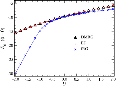
Figure 3: (Color online) Ground state energies at $\phi=0$ calculated by DMRG (filled triangles), ED (open circles), and fRG (crosses) as functions of $U$ within the Luttinger liquid regime for $L=16$ and $V=1$.

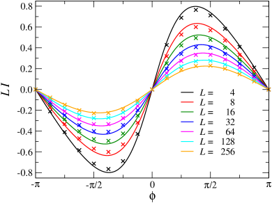
Figure 4: (Color online) Persistent currents calculated by fRG (lines) and DMRG (symbols $\times$) at half-filling for $U=1$, $V=2$, and various ring lengths $L$. The currents with the largest amplitude correspond to $L=4$ and then the amplitudes decrease with increasing $L$.

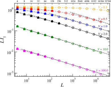
Figure 5: (Color online) The first Fourier coefficient $I_{1}$ versus the length of the ring $L$ for $U=1$ and various $V$. The open circles and the filled triangles, respectively, correspond to the fRG and DMRG data. The dashed straight lines show the asymptotics $\alpha_{\rm B}=\frac{1}{3}$. The upper $x$-axis shows the exact number of the sites $L$ at which the calculations were performed.

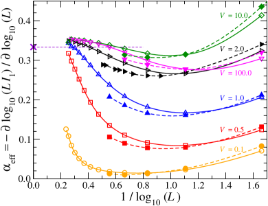
Figure 6: (Color online) The effective exponent $\alpha_{\rm eff}$ versus the inverse of $\log_{10}(L)$ for the interaction $U=1$ and various impurities $V$. The open and filled symbols correspond to fRG and DMRG data, respectively.

V.1 fRG and DMRG analysis at half-filling

Figure 4 shows persistent currents as functions of the flux calculated at half-filling ($n=\frac{1}{2}$) using DMRG and fRG for various ring lengths $L$ and for an intermediate impurity strength $V=2$ (corresponding to transmission $T=\frac{1}{2}$). The data indicate that for small and intermediate ring lengths $L$, the DMRG and fRG calculations agree rather well. DMRG calculations are hardly feasible for $L>256$, and only fRG data are available in order to study the large $L$ limit.

Bosonization theory including additional approximations predict a power law decay of the persistent current at large $L$, cf. Eq. (11). In Fig. 5 we compare this asymptotic decay (dashed lines) with the numerically determined first Fourier coefficient of the persistent current $LI_{1}$ in a logarithmic plot. From Bosonization one expects that $LI_{1}$ decays asymptotically as $L^{-\alpha_{\rm B}}$. The open circles represent the fRG data and the filled triangles the DMRG results. Again we see the good agreement between both methods, and it is obvious that the asymptotic decay does not depend on the impurity strength (if at least $V>0.1$), which ranges from rather weak $V=0.1$ ($T=0.9975$) to very strong $V=100$ ($T=0.0004$). The asymptotic regime is reached at smaller $L$ for stronger impurities.

Notice a tiny deviation of the fRG data from the dashed lines with the common power-law exponent $\alpha_{\rm B}$ at large $L$. This is due to the approximations involved in the fRG method and is known from studies of quantum wires Enss . However, there are also numerical limitations: for large systems the differences between currents calculated for different magnetic fluxes are so tiny that they can not be resolved by the floating point data representation of the computer, and the current cannot be calculated reliably. This numerical limitation also prevents us to calculate even larger systems.

In order to quantify the deviation of the numerical data from the expected power law, we define an effective exponent

$$\alpha_{\rm eff}=-\frac{\partial\log_{10}(LI_{1})}{\partial\log_{10}(L)}\,,$$ (22)

which is shown in Fig. 6 as a function of $1/\log_{10}(L)$. The data labeled by the open and filled symbols are obtained from the fRG and DMRG results shown in Fig. 5 using a numerical derivative. If the impurity is weak ($V=0.1$), the effective exponent $\alpha_{\rm eff}$ deviates significantly from $\alpha_{\rm B}=\frac{1}{3}$ (the horizontal dashed line). It is expected that substantially larger systems would need to be considered to approach the asymptotics in this case. For $V\geq 0.5$, the numerically determined exponents tend to saturate at $\alpha_{\rm eff}\approx 0.35$ which is about 5% larger than the expected $\alpha_{\rm B}=\frac{1}{3}$. Our result is in good agreement with the leading $U$-behavior, where the correction to the exponent for the quantum wire is known to be $\frac{U}{\pi}=0.318$ Enss . As already stated, we attribute this deviation to the approximations involved in the fRG. Similar results were obtained in a study on open chains AND04 , where the same power law decay is extracted from the decay of the spectral weight near the impurity site.

From our data analysis it emerges that the effective exponents for larger $L$ are also non-negligibly influenced by the numerical limitations discussed above, which are seen in the figure as small irregularities in the approach of the numerical data to saturation. Notice that we are dealing with extremely tiny effects observed in the exponent $\alpha_{\rm eff}$. Thus, extremely accurate calculations of the ground state energy is the key to the analysis of the effective exponent. There is another feature of the effective exponent worth mentioning: it shows a characteristic minimum at lengths $8\lesssim L\lesssim 100$ within the range of $V$.

The effective exponent determined from the DMRG data (full symbols) is systematically below the fRG results for all but the very small systems. Since the DMRG data are expected to be accurate, one may conjecture that $\alpha_{\rm eff}$ approaches $\alpha_{\rm B}=\frac{1}{3}$ for $L\to\infty$, if DMRG calculations for such large systems would be feasible.

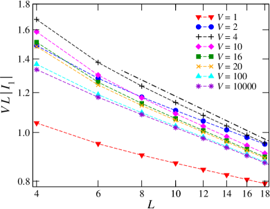
Figure 7: (Color online) The persistent current versus $L$ for a variety of $V$’s obtained by ED at $U=1$ and half-filling.

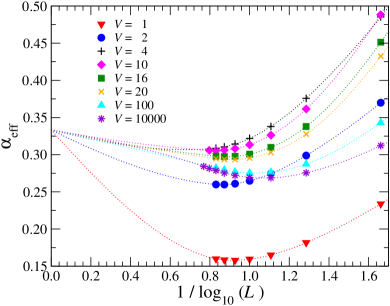
Figure 8: (Color online) Dependence of the effective exponent on $1/\log_{10}(L)$ for the same parameters as in Fig. 7.

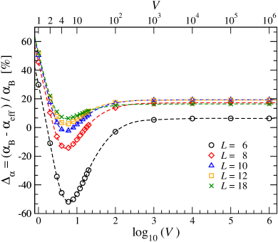
Figure 9: (Color online) Relative difference between the effective and asymptotic exponents as a function of the impurity strength $V$ for several sizes $L$.

V.2 Non-monotonous behavior of the effective exponent

Another interesting feature can be seen in Fig. 6. Both fRG and DMRG data show that the result for the strongest impurity $V=100$ appears to be out of sequence if compared to the other $V$’s. To elucidate this further, we performed a series of calculations using ED at smaller sizes $L$. Figure 7 shows the first Fourier coefficient of the persistent current $I_{1}$ as a function of $L$ on a logarithmic scale for on-site impurities in the range $1\leq V\leq 10^{4}$. In order to gather the data, the Fourier coefficient is scaled with $VL$ in Fig. 7. Furthermore, we plot the absolute value of the Fourier coefficient in order to remove the even-odd effect discussed in Section II. The straight dot-dashed line corresponds to $\alpha_{\rm B}=\frac{1}{3}$.

Figure 8 shows corresponding calculations of the effective exponent $\alpha_{\rm eff}$ for the same set of impurity strengths. The dotted lines only serve as guides to the eye and should not be taken as extrapolations. Again, it is obvious that the data for the cases $V\geq 10^{2}$ appear to be out of sequence as in Fig. 6. In Fig. 9 we plot the relative difference $\Delta_{\alpha}=(\alpha_{\rm B}-\alpha_{\rm eff})/\alpha_{\rm B}$ in order to quantify the dependence of the effective exponent on the impurity strength $V$ for several system sizes $L$. A minimum of $\Delta_{\alpha}$ appears at $V\approx 4$ for $U=1$. We, therefore, identify three regions in the figure (for reachable system sizes): in the first region, $0<V\lesssim 4$, we observe the standard behavior, i.e., the stronger the impurity, the faster the convergence of $\alpha_{\rm eff}$ to $\alpha_{\rm B}$. In the the second region which starts at around $V\approx 4$ and ends around $V=10^{3}$, this behavior is reversed. In the third region $V>10^{3}$ the effective exponent $\alpha_{\rm eff}$ saturates and does not change any more with increasing impurity strength.

V.3 DMRG study at low fillings

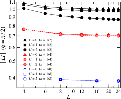
Figure 10: (Color online) Persistent currents as a function of the system size $L$ for magnetic flux $\phi=\frac{\pi}{2}$, various electron concentrations $n$, and interactions $U$. Plotted is the absolute value of the persistent current in order to remove the sign change between even and odd electron fillings.

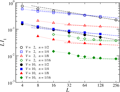
Figure 11: (Color online) Persistent currents versus system size $L$ for $U=1$ at various electron fillings $n$. The open and full symbols correspond to the impurity $V=2$ and $V=10$, respectively. The slopes of the dashed lines coincide with the asymptotic exponents $\alpha_{\rm B}$.

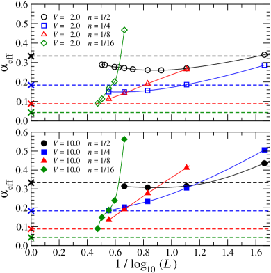
Figure 12: (Color online) The effective exponents versus the inverse of $\log_{10}(L)$ for the data displayed in Fig. 11. The horizontal dashed lines correspond to the asymptotic exponents $\alpha_{\rm eff}(n)$ with $n$ as listed in the legend.

Studies of the persistent current at low fillings try to address the question of differences between discrete lattice models and continuous models of one-dimensional systems. Such questions have been addressed in a recent comprehensive numerical study Nemeth ; Krcmar . Discrete models mimic continuous electron gas models if the electron concentration $n$ is such that the cosine dispersion of the discrete system can reasonably well approximate the parabolic dispersion of the electron gas. Moreover, lattice models violate Galilean invariance Schick . In a Galilean invariant model without impurity ($V=0$) the persistent current should not depend on the interaction $U$.

First we check whether the interaction dependence of the current really disappears at lower fillings: Figure 10 shows persistent currents as a function of system size $L$ for $U=0$, $U=1$, and $U=2$ at various fillings $n=\frac{1}{2}$, $\frac{1}{4}$, and $\frac{1}{8}$. The currents at half-filling (full symbols) strongly depend on the electron-electron interaction, while the electron gas is better approximated at quarter-filling (shaded symbols). A negligibly small dependence on $U$ is found at $n=\frac{1}{8}$ (open symbols) where Galilean invariance is almost satisfied.

Figure 11 shows the decay of the persistent current as a function of the ring size $L$ for electron concentrations $n=\frac{1}{2}$, $\frac{1}{4}$, $\frac{1}{8}$, and $\frac{1}{16}$ on a logarithmic scale for $V=2$ (open symbols) and $V=10$ (full symbols). The asymptotic values $\alpha_{\rm B}(n)$ expected from the Bosonization analysis Haldane ; Qin ; And are indicated by the dashed straight lines corresponding to exponents $\alpha_{\rm B}(n=\frac{1}{2})=\frac{1}{3}$, $\alpha_{\rm B}(\frac{1}{4})=0.18383$, $\alpha_{\rm B}(\frac{1}{8})=0.08825$, $\alpha_{\rm B}(\frac{1}{16})=0.042940$. On the scale of the figure the data seemingly reach the asymptotics. A more detailed picture of how the effective power-law exponents $\alpha_{\rm eff}$ approach the expected asymptotic values $\alpha_{\rm B}$ is shown in Fig. 12. The upper and lower panels show the effective exponent calculated for $V=2$ and $V=10$, respectively, at various fillings $n$. It is obvious that the $\alpha_{\rm eff}(n)$ do not converge to $\alpha_{\rm B}(n)$, and substantially larger system sizes $L$ would need to considered in order to see convergence. From our data we, therefore, cannot support the suggestion Nemeth ; Krcmar that the asymptotic regime can be reached at a small number of electrons $nL$ in continuous models.

VI Summary

We studied the asymptotic power law decay of persistent currents using three different numerical methods (fRG, DMRG, ED). To this end we improved the fRG method so that systems with up to $3\cdot 10^{4}$ sites could be treated. We used DMRG and ED in order to benchmark the fRG results and confirmed a sufficiently good agreement between fRG, DMRG, and ED calculations. We confirmed that the fRG is a suitable method for extracting the asymptotic Luttinger power law exponent $\alpha_{\rm B}$.

We found that $\alpha_{\rm B}$ which describes the decay of the persistent current is about 5% overestimated by the fRG results compared to expectations from Bosonization and additional approximation. This deviation we attribute to the approximation of the fRG method, and the effective exponent is known to be correct to the leading order in the electron-electron interaction from the calculations of the same exponent for quantum wires. The accurate DMRG analysis cannot, unfortunately, be extended to sufficiently large systems. However, there are indications that the expected asymptotic values could be reached, if larger systems could be calculated. It is found that the effective exponent for a fixed impurity strength $V$ shows a typical minimum for lengths $8\lesssim L\lesssim 100$ at half-filling.

Generally, it is known that the stronger the impurity, the faster the asymptotic regime is reached. However, we identified three regions for $U=1$: in the first region, $0<V\lesssim 4$, we observed the standard behavior. (The case $V=4$ corresponds to $T=\frac{1}{5}$.) In the the second region $4\lesssim V\lesssim 10^{3}$ this behavior is reversed. In the third region $V>10^{3}$ the dependence of the effective exponent $\alpha_{\rm eff}$ on the impurity strength $V$ saturates.

Since discrete lattice models are not Galilean invariant, we decreased the electron filling down to $n=\frac{1}{16}$ such that the discrete Hamiltonian mimics a continuous electron gas with a quadratic dispersion law. From our data we see that even at low fillings, i.e. for quasi-continuous models, we need large systems in order to reach the expected power law exponents.

Appendix A Solution of the fRG equations for large $k$

Here we show how the initial conditions given in Eqs. (III) are determined. We start from the equations (III) for the coefficients $a_{k}$ for large $k$

$$a_{k,jj}^{\prime}=\frac{2U}{\pi}\frac{\sin(k~{}0^{+})}{k},\quad a_{k,j(j\pm 1)}^{\prime}=0,$$ (23)

noting that $U_{k}=U$ for large $k$ ($0^{+}$ denotes a positive infinitesimal increment). This equation is easily solved using the initial conditions at $k=\infty$ given in Eq. (III) with the result

$$a_{k,jj} = -U\left(1-\frac{2}{\pi}{\rm Si}(k~{}0^{+})\right)\delta_{jj}-V\delta_{j1}+\mu\delta_{jj},$$

$$\quad a_{k,j(j\pm 1)} = 0.$$ (24)

Here, ${\rm Si}(z)$ is the sine integral function. The impurity with strength $V$ is placed at site $j=1$. This result can now be used in order to solve the equation for $a_{k,0}$ for large k,

$$a_{k,0}^{\prime}=\frac{L\mu-V}{\pi}\frac{\sin(k~{}0^{+})}{k}-\frac{LU}{\pi}\frac{\sin(k~{}0^{+})}{k}\left(1-\frac{2}{\pi}{\rm Si}(k~{}0^{+})\right)$$ (25)

where the expansion $\ln(1+x)\approx x$ for $x<1$ has been used. Integration of Eq. (25) yields

$$a_{k,0}=\frac{V}{2}+\frac{L}{2}\left(\frac{U}{2}-\mu\right).$$ (26)

where the limit $0^{+}\rightarrow 0$ has been performed.

Appendix B Numerical solution of the flow equations for the self energies and the ground state energy

The solution of the flow equations for the self-energies and ground state energy (III) requires the calculation of the inverse and determinant of (potentially) large cyclic tridiagonal matrices at each step of the integration of a set of ordinary differential equations. Of course, this could be achieved with standard library routines. However, due to the special form of the Eqs. (III) we only need to determine the cyclic tridiagonal part of these matrices. Therefore, in the following we will develop methods adapted to our special needs. As a consequence we achieve a significant speed-up of the numerical calculation as well as considerable reduction of the computer memory requirements. Such improvements enable us to treat large system sizes.

B.1 Inversion of cyclic tridiagonal matrices

For matrices $\mathbf{M}$ which can be represented as the sum of a tridiagonal matrix $\mathbf{T}$ and a direct product of two vectors $\mathbf{u}$ and $\mathbf{v}$,

$$\mathbf{M}=\mathbf{T}+\mathbf{u}\otimes\mathbf{v},$$ (27)

the inverse can be obtained using the Sherman-Morrison formula rec

$$\mathbf{M}^{-1}=\mathbf{T}^{-1}-\frac{\mathbf{z}\otimes\mathbf{w}}{1+\mathbf{v}\cdot\mathbf{z}}$$ (28)

with

$$\mathbf{z}=\mathbf{T}^{-1}\mathbf{u},\quad\quad\quad\mathbf{w}=(\mathbf{T}^{-1})^{T}\mathbf{v}.$$ (29)

A general cyclic tridiagonal matrix

$$\mathbf{M}=\left(\begin{array}[]{ccccc}a_{1}&b_{1}&0&\cdots&c_{1}\\ c_{2}&a_{2}&b_{2}&&0\\ 0&\ddots&\ddots&\ddots&\vdots\\ \vdots&&c_{n-1}&a_{n-1}&b_{n-1}\\ b_{n}&\cdots&0&c_{n}&a_{n}\end{array}\right)$$ (30)

can be written in the form (27) with the tridiagonal part $\mathbf{T}$ given by

$$\mathbf{T}=\left(\begin{array}[]{ccccc}\alpha_{1}&b_{1}&0&\cdots&0\\ c_{2}&\alpha_{2}&b_{2}&&0\\ 0&\ddots&\ddots&\ddots&\vdots\\ \vdots&&c_{n-1}&\alpha_{n-1}&b_{n-1}\\ 0&\cdots&0&c_{n}&\alpha_{n}\end{array}\right)$$ (31)

with $\alpha_{1}=2a_{1}$, $\alpha_{n}=a_{n}+c_{1}b_{n}/a_{1}$ and $\alpha_{i}=a_{i}$ for $1<i<n$. The vectors $\mathbf{u}$ and $\mathbf{v}$ are defined by

$$\mathbf{u}=\left(-a_{1},0,\cdots,0,b_{n}\right),\quad\mathbf{v}=\left(1,0,\cdots,0,-c_{1}/a_{1}\right).$$ (32)

For the inversion of the tridiagonal part $\mathbf{T}$, we use a method inspired by Andergassen et al. And , which is based on Ref. meu . However, in our case the tridiagonal matrix is not complex symmetric, therefore, we have to use an $\mathbf{LU}$ decomposition of $\mathbf{T}$ instead of the $\mathbf{LDU}$ decomposition employed in Ref. And . Details are described in the following subsection.

B.2 Implementation

According to Eq. (28) the inversion of a general cyclic tridiagonal matrix requires two essential steps: (i) the inversion of a tridiagonal matrix and (ii) the determination of the vectors $\mathbf{z}$ and $\mathbf{w}$.

(i) A tridiagonal matrix can be represented as a product of two matrices $\mathbf{T}=\mathbf{LU}=\tilde{\mathbf{U}}\tilde{\mathbf{L}}$, where $\mathbf{U}$, $\tilde{\mathbf{U}}$ are upper diagonal and $\mathbf{L}$, $\tilde{\mathbf{L}}$ are lower diagonal matrices. From the $\mathbf{L}\mathbf{U}$ decomposition

$$\mathbf{T}=\mathbf{L}\mathbf{U}=$$ (33)

$$\left(\begin{array}[]{ccccc}d_{1}&&&&\\ c_{2}&d_{2}&&\\ &\ddots&\ddots&&\\ &&c_{n-1}&d_{n-1}&\\ &&&c_{n}&d_{n}\end{array}\right)\left(\begin{array}[]{ccccc}1&u_{1}&&&\\ &1&u_{2}&\\ &&\ddots&\ddots&\\ &&&1&u_{n-1}\\ &&&&1\end{array}\right)$$ (44)

with

$$d_{1}=\alpha_{1},\quad d_{i}=\alpha_{i}-u_{i-1}c_{i},\quad u_{i}=b_{i}/d_{i}$$ (45)

one easily finds for $1<i<j<n$ the relations

$$(\mathbf{T}^{-1})_{n,n}=1/d_{n},\quad(\mathbf{T}^{-1})_{i,j}=-u_{i}(\mathbf{T}^{-1})_{i+1,j}.$$ (46)

Similarly, from the $\tilde{\mathbf{U}}\tilde{\mathbf{L}}$ decomposition of $\mathbf{T}$,

$$\mathbf{T}\!=\!\tilde{\mathbf{U}}\tilde{\mathbf{L}}=$$ (47)

$$\left(\begin{array}[]{ccccc}1&\tilde{u}_{1}&&&\\ &1&\tilde{u}_{2}&\\ &&\ddots&\ddots&\\ &&&1&\tilde{u}_{n-1}\\ &&&&1\end{array}\right)\!\!\left(\begin{array}[]{ccccc}\tilde{d}_{1}&&&&\\ c_{2}&\tilde{d}_{2}&&\\ &\ddots&\ddots&&\\ &&c_{n-1}&\tilde{d}_{n-1}&\\ &&&c_{n}&\tilde{d}_{n}\end{array}\right)$$ (58)

with

$$\tilde{d}_{n}=\alpha_{n}\quad\tilde{d}_{i}=\alpha_{i}-\tilde{u}_{i}c_{i+1}\quad\tilde{u}_{i}=b_{i}/\tilde{d}_{i+1},$$ (59)

one obtains for $1<i<j<n$ the relations

$$(\mathbf{T}^{-1})_{1,1}=1/\tilde{d}_{1},\quad(\mathbf{T}^{-1})_{i,j}=-\tilde{u}_{j-1}(\mathbf{T}^{-1})_{i,j-1}.$$ (60)

Combining Eqs. (46) and (60) yields a recursion relation for the diagonal elements of $\mathbf{T}^{-1}$

$$(\mathbf{T}^{-1})_{i+1,i+1}=\frac{\tilde{u}_{i}}{u_{i}}(\mathbf{T}^{-1})_{i,i}$$ (61)

with the initial condition given in Eq. (60). From the diagonal elements one then generates the upper diagonal as well as the upper corner element using the relations given above. Alternatively, the $\tilde{\mathbf{U}}\tilde{\mathbf{L}}$ decomposition yields the relation

$$(\mathbf{T}^{-1})_{i,j}=-\frac{c_{i}}{\tilde{d}_{i}}(\mathbf{T}^{-1})_{i-1,j}~{}~{}~{}~{}{\rm for}~{}1<j<i<n,$$ (62)

which is used to generate the lower diagonal and corner element, respectively.

(ii) The vector $\mathbf{z}$ is obtained from Eq. (29), $\mathbf{Tz}=\mathbf{LUz}=\mathbf{u}$, as follows: first we solve recursively $\mathbf{L}\mathbf{z}^{\prime}=\mathbf{u}$ for $\mathbf{z}^{\prime}$

$$z_{1}^{\prime}=u_{1}/d_{1},\quad z^{\prime}_{i}=(u_{i}-c_{i}z^{\prime}_{i-1})d_{i}~{}~{}~{}~{}{\rm for}~{}1<i\leq n,$$ (63)

and then obtain $\mathbf{z}$ recursively from $\mathbf{U}\mathbf{z}=\mathbf{z}^{\prime}$

$$z_{n}=z_{n}^{\prime},\quad z_{i}=z_{i}^{\prime}-u_{i}z_{i+1}~{}~{}~{}~{}{\rm for}~{}1\leq i<n.$$ (64)

In a similar way one determines $\mathbf{w}$ from $\mathbf{T}^{T}\mathbf{w}=\mathbf{v}$.

B.3 Determinant of a cyclic tridiagonal matrix

The determinant of a cyclic tridiagonal matrix is calculated using a formula given in Ref. moli

$$\det\left(\begin{array}[]{ccccc}a_{1}&b_{1}&0&\cdots&c_{1}\\ c_{2}&a_{2}&b_{2}&&0\\ 0&\ddots&\ddots&\ddots&\vdots\\ \vdots&&c_{n-1}&a_{n-1}&b_{n-1}\\ b_{n}&\cdots&0&c_{n}&a_{n}\end{array}\right)=$$ (70)

$$\quad(-1)^{n+1}\left(\prod_{i=1}^{n}b_{i}+\prod_{i=1}^{n}c_{i}\right)+{\rm Tr}\prod_{i=1}^{n}\left(\begin{array}[]{cc}a_{i}&-b_{i-1}c_{i}\\ 1&0\end{array}\right)$$ (73)

with $b_{0}=b_{n}$. For large systems, the products in this formula can easily underflow or overflow. This must be carefully controlled appropriately.

References

References

- (1) B.S. Deaver Jr. and W. M. Fairbank. Phys. Rev. Lett., 7:43, 1961.
- (2) N. Byers and C. N. Yang. Phys. Rev. Lett., 7:46, 1961.
- (3) M. Büttiker, Y. Imry, and R. Landauer. Phys. Lett., 96A:365, 1983.
- (4) L.P. Lévy, G. Dolan, J. Dunsmuir, and H. Bouchiat. Phys. Rev. Lett., 64:2074, 1990.
- (5) V. Chandrasekhar, R. A. Webb, M. J. Brady, M. B. Ketchen, W. J. Gallagher W J, and A. Kleinsasser. Phys. Rev. Lett., 67:3578, 1991.
- (6) D. Mailly, C. Chapelier, and A. Benoit. Phys. Rev. Lett., 70:2020, 1993.
- (7) B. Reulet, M. Ramin, H. Bouchiat, and D. Mailly D. Phys. Rev. Lett., 75:124, 1995.
- (8) E. M. Q. Jariwala, P. Mohanty, M. B. Ketchen, and R. A. Webb. Phys. Rev. Lett., 86:1594, 2001.
- (9) W. Rabaout, L. Saminadayar, D. Mailly, K. Hasselbach, A. Benot, and B. Etienne. Phys. Rev. Lett., 86:3124, 2001.
- (10) N. A. J. M. Kleemans et al. Phys. Rev. Lett., 99:146808, 2007.
- (11) H. Bouchiat. Physics, 1:7, 2008.
- (12) R. Landauer and M. Büttiker. Phys. Rev. Lett., 54:2049, 1985.
- (13) H. F. Cheung, Y. Gefen, E. K. Riedel, and W. H. Shih. Phys. Rev. B, 37:6050, 1988.
- (14) M. Abraham and R. Berkovits. Phys. Rev. Lett., 70:1509, 1993.
- (15) G. Bouzerar, D. Poiblanc, and G. Montambaux. Phys. Rev. B, 49:8258, 1994.
- (16) A. O. Gogoglin and Prokof’ev. Phys. Rev. B, 50:4921, 1994.
- (17) H. Kato and D. Yoshioka. Phys. Rev. B, 50:4943, 1994.
- (18) A. Cohen, K. Richter, and R. Berkovits. Phys. Rev. B, 57:6223, 1998.
- (19) M. Henkel and D. Karevski. Eur. Phys. J. B, 5:787, 1998.
- (20) S. Jaimungal, M. H. S. Amin, and G. Rose. Int. J. Mod. Phys. B, 13:3171, 1999.
- (21) V. Meden and U. Schollwöck. Phys. Rev. B, 67:035106, 2003.
- (22) T. Enss, V. Meden, S. Andergassen, X. Barnabé-Thériault, W. Metzner, and K. Schönhammer. Phys. Rev. B, 71:155401, 2005.
- (23) S. Friederich and V. Meden. Phys. Rev. B, 77:195122, 2008.
- (24) H. Bary-Soroker, O. Entin-Wohlmann, and Y. Imry. Phys. Rev. Lett., 101:057001, 2008.
- (25) J. Heinrichs. J. Phys.: Condens. Matter, 20:345232, 2008.
- (26) B. L. Altshuler, Y. Gefen, and Y. Imry Y. Phys. Rev. Lett., 66:88, 1991.
- (27) V. Ambegaokar and U. Eckern. Europhys. Lett., 13:733, 1990.
- (28) E. Gambetti-Césare, D. Weinmann, R. A. Jalabert, and Ph. Brune. Eurphys. Lett., 60:120, 2005.
- (29) E. Gambetti. Phys. Rev. B, 72:165338, 2005.
- (30) R. Krčmár, A. Gendiar, M. Moško, R. Németh, P. Vagner, and L. Mitas. Physica E, 40:1507, 2008.
- (31) R. Németh, M. Moško, R. Krčmár, A. Gendiar, M. Indlekofer, and L. Mitas. arXiv:0902.2225.
- (32) A. Luther and I. Peschel. Phys. Rev. B, 9:2911, 1974.
- (33) W. Apel and T. M. Rice. Phys. Rev. B, 26:7063, 1982.
- (34) C. L. Kane and M. P. A. Fisher. Phys. Rev. Lett., 68:1220, 1992.
- (35) C. L. Kane and M. P. A. Fisher. Phys. Rev. B, 46:15233, 1992.
- (36) F. D. M. Haldane. Phys. Rev. Lett., 45:1358, 1980.
- (37) K. A. Matveev, D. Yue, and L. I. Glazmann. Phys. Rev. Lett., 71:3351, 1993.
- (38) D. Yue, L. I. Glazmann, and K. A. Matveev. Phys. Rev. B, 49:1966, 1994.
- (39) J. Polchinski. Nucl. Phys. B, 231:269, 1984.
- (40) C. Wetterich. Phys. Lett. B, 301:90, 1993.
- (41) T. R. Morris. Int. J. Mod. Phys. A, 9:2411, 1994.
- (42) M. Salmhofer. Commun. Math. Phys., 194:249, 1998.
- (43) M. Salmhofer and C. Honerkamp. Prog. Theor. Phys., 105:1, 2001.
- (44) S. R. White. Phys. Rev. Lett., 69:2863, 1992.
- (45) S. R. White. Phys. Rev. B, 48:10345, 1993.
- (46) I. Peschel, X. Wang, M. Kaulke, and K. Hallberg (Eds.). Lecture Notes in Physics 528 Density-Matrix Renormalization, A New Numerical Method in Physics. Springer, Berlin, 1999.
- (47) U. Schollwöck. Rev. Mod. Phys., 77:259, 2005.
- (48) R. E. Peierls. Z. Phys. B: Condens. Matter, 80:763, 1933.
- (49) V. Meden, P. Schmitteckert, and N. Shannon. Phys. Rev. B, 57:8878, 1998.
- (50) S. Andergassen, T. Enss, V. Meden, W. Metzner, U.Schollwöck, and K. Schönhammer. Phys. Rev. B, 70:075102, 2004.
- (51) V. Meden, W. Metzner, U. Schollwöck, and K. Schönhammer. Phys. Rev. B, 65:045318, 2002.
- (52) V. Meden, W. Metzner, U. Schollwöck, and K. Schönhammer. J. Low Temp. Phys., 126:1147, 2002.
- (53) S. Andergassen, T. Enss, V. Meden, W. Metzner, U. Schollwöck, and K. Schönhammer. Phys. Rev. B, 70:075102, 2004.
- (54) M. Weyrauch and D. Sibold. Phys. Rev. B, 77:125309, 2008.
- (55) J. Berges, N. Tetradis, and C. Wetterich. Phys. Rep., 363:223–386, 2002.
- (56) M. Schick. Phys. Rev., 166:144, 1967.
- (57) S. Qin, M. Fabrizio, L. Yu, M. Oshikawa, and I. Affleck. Phys. Rev. B, 56:9766, 1997.
- (58) S.A. Teukolsky, W. T. Vetterling, and B.P.Flannery. Numerical Recipes in Fortran 77. Cambrige University Press, Cambridge, MA, 1986.
- (59) G. Meurant. SIAM J. Matrix Anal. Appl., 13:707, 1992.
- (60) L. G. Molinari. arXiv:0712.0681v3.