Coulomb-gauge ghost and gluon propagators in $\boldsymbol{SU(3)}$ lattice Yang-Mills theory

Abstract

We study the momentum dependence of the ghost propagator and of the space and time components of the gluon propagator at equal time in pure $SU(3)$ lattice Coulomb gauge theory carrying out a joint analysis of data collected independently at RCNP Osaka and Humboldt University Berlin. We focus on the scaling behavior of these propagators at $\beta=5.8,\ldots,6.2$ and apply a matching technique to relate the data for the different lattice cutoffs. Thereby, lattice artifacts are found to be rather strong for both instantaneous gluon propagators at large momentum. As a byproduct we obtain the respective lattice scale dependences $a(\beta)$ for the transversal gluon and the ghost propagator which indeed run faster with $\beta$ than two-loop running, but slightly slower than what is known from the Necco-Sommer analysis of the heavy quark potential. The abnormal $a(\beta)$ dependence as determined from the instantaneous time-time gluon propagator, $D_{44}$, remains a problem, though. The role of residual gauge-fixing influencing $D_{44}$ is discussed.

I Introduction

Lattice investigations of the gluon and ghost propagator have become an important topic over the last ten years after the pioneering lattice studies in the Landau gauge appeared in the late eighties and nineties Mandula and Ogilvie (1987); Marenzoni et al. (1995); Suman and Schilling (1996); Nakamura et al. (1995); Leinweber et al. (1998); Becirevic et al. (1999); Mandula (1999) and after the coupled solutions to the corresponding Dyson-Schwinger equations in the deep infrared momentum region were found von Smekal et al. (1997, 1998). Since then, the available amount of lattice data on these propagators has grown (see, e.g., Bonnet et al. (2000, 2001); Bowman et al. (2004); Sternbeck et al. (2005); Ilgenfritz et al. (2007); Sternbeck et al. (2006, 2007); Bogolubsky et al. (2007); Bowman et al. (2007); Kamleh et al. (2007); Cucchieri and Mendes (2007)) and also studies based on functional methods have made considerable progress Lerche and von Smekal (2002); Zwanziger (2002); Pawlowski et al. (2004); Fischer and Pawlowski (2007) such that in Landau gauge one is nowadays in the comfortable situation to confront continuum results with a broad set of independent lattice data (see, e.g., Fischer et al. (2008); Sternbeck and von Smekal (2008) for recent discussions).

In Coulomb gauge, comparably few lattice investigations of the aforementioned propagators have been performed. For example, Langfeld and Moyaerts Langfeld and Moyaerts (2004) as well as Cucchieri and Zwanziger Cucchieri and Zwanziger (2002), and very recently also Burgio, Quandt and Reinhardt Quandt et al. (2007); Burgio et al. (2008) have carried out such computations for the gauge group $SU(2)$. In fact, the Coulomb gauge provides an interesting alternative to the Landau gauge since the resulting Hamiltonian approach allows to apply the variational principle to get analytic results for the QCD vacuum wave functional and for the spectrum of hadronic bound states. This approach has been mainly pursued by the Tübingen group Reinhardt and Feuchter (2005) in recent years. Their investigations of (truncated) systems of Dyson-Schwinger equations in the Coulomb gauge provided various solutions in the infrared, including also asymptotic “conformal” or “scaling” solutions that are characterized in the infrared by a singular power-law behavior of the ghost propagator and a powerlike vanishing transversal gluon propagator Schleifenbaum et al. (2006); Epple et al. (2006, 2008), very similar to what was found in Landau gauge.

Among us, the authors from Japan have done several lattice investigations before, concentrating on the Coulomb gauge for $SU(3)$ gauge fields. The instantaneous gluon propagators and the ghost propagator were computed in Nakagawa et al. (2007a), and correlators of incomplete Polyakov-loops were also determined. The latter was studied in order to interpolate between the confinement potential $V_{c}$ (derived from Wilson loops) and the Coulomb potential $V_{\mathrm{Coul}}$ (known to restrict $V_{c}$ from above Zwanziger (1998, 2003)). Furthermore, it was possible in this way to extract potentials for the quark-antiquark singlet and octet channels, as well as for the quark-quark symmetric sextet and antisymmetric anti-triplet channels Nakagawa et al. (2006, 2008). The eigenvalue spectrum of the Coulomb-gauge Faddeev-Popov (FP) operator was studied in Greensite et al. (2005); Nakagawa et al. (2007b).

Recently, some of us have also computed the gluon and ghost propagators as well as the Coulomb potential $V_{\mathrm{Coul}}$, the latter directly from the FP operator, however Voigt et al. (2007). For $V_{\mathrm{Coul}}$ very strong Gribov-copy effects were reported, and it still remains difficult to give a final answer for the infrared momentum limit Voigt et al. (2008). Independent of that, the factorization assumption proposed in Zwanziger (2004) relating $V_{\mathrm{Coul}}$ to the square of the ghost propagator was found to be strongly violated at low momenta.

In this paper we present a joint analysis of data from Berlin and Osaka for the instantaneous propagators of both ghost and gluons. For the transverse gluon propagator as well as for the ghost propagator similar infrared properties as for the Landau gauge are expected also for the Coulomb gauge. In Landau gauge, e.g., a gluon propagator vanishing in the zero-momentum limit (or a infrared-diverging ghost dressing function) is crucial from the point of view of the Gribov-Zwanziger confinement scenario Gribov (1978); Zwanziger (1991) or the Kugo-Ojima confinement criterion Kugo and Ojima (1979). In Coulomb gauge, the instantaneous time-time gluon correlator should become singular and be related to the effective Coulomb potential.

This study provides a comprehensive set of lattice data on the instantaneous gluon and ghost propagators in the Coulomb gauge of pure $SU(3)$ lattice gauge theory. We discuss their momentum dependence and analyze in detail apparent scaling violations of the space and time components of the gluon propagator. We show that these violations can be ameliorated if different cuts are applied on the data. In fact, they are effectively eliminated by a matching procedure that provides us also with the running of the lattice scale $a(\beta)$, separately for each propagator. With the exception of the time-time propagator $D_{44}$, we find these runnings to be in good agreement with other prescriptions. The behavior of the renormalization coefficients, that are also provided by the matching procedure, is smooth a long as $\beta\geq 6.0$.

The structure of the paper is as follows: In Sect. II we describe the setup of our lattice simulation including details on our gauge-fixing algorithms. Sect. III introduces the relevant lattice observables. The data for the propagators is discussed in Sect. IV where we report on obvious scaling violations for the gluon propagators. We then use a matching procedure to relate the propagators for different lattice cutoffs to each other and discuss the outcome of this for the instantaneous gluon propagators and the ghost propagator in Sects. V, VI and VII. We present in detail the interplay of the matching procedure with the necessity of an additional momentum cutoff that restricts the reliability of the data to relatively small momenta $|pa|<\alpha$. The lattice scale dependence $a(\beta)$, as determined thereby, is compared to what is known from the literature in Sect. VIII. Finally, in Sect. IX, we discuss the momentum dependence of the propagators in both the ultraviolet and infrared region. We draw our conclusions in Sect. X. To make the paper self-consistent, we give a brief outline of the matching procedure for the Coulomb-gauge propagators in Appendix A. Fit and matching tables are presented in Appendix B.

II Lattice field ensembles and gauge fixing

The results discussed below are based on an extensive set of quenched gauge configurations generated in Osaka and Berlin. At both places we employed Wilson’s one-plaquette action and a standard heatbath algorithm (including microcanonical steps) for thermalization, but used different values of the inverse coupling $\beta$ and different lattice sizes $L^{4}$. Those, together with a couple of other useful parameters, are listed in Table 1 that can be found in Appendix B.

In our analysis below we combine the data from Osaka with the data obtained in Berlin. Both sets are nicely consistent with each other as we checked by comparing data at $\beta=5.8$ and $6.0$.

Configurations were fixed to Coulomb gauge via maximizations of the Coulomb gauge functional

$$F_{U}[g]=\sum_{i=1}^{3}\sum_{\vec{x},t}\frac{1}{3}\operatorname{\mathfrak{Re}}\operatorname{Tr}U^{g}_{i}(\vec{x},t)\,,$$ (1)

where $U^{g}_{i}(\vec{x},t)=g(\vec{x},t)\,U_{i}(\vec{x},t)\,g^{\dagger}(\vec{x}+\hat{i},t)$. For a fixed $U$ this was done by iteratively changing $g$ using a standard overrelaxation (OR) algorithm in Osaka and the simulated annealing method combined with subsequent overrelaxation (SA+OR) as in Refs. Voigt et al. (2007, 2008) in Berlin. Strictly speaking, different gauge-fixing methods may cause variations in the data of gauge-variant observables due to the Gribov ambiguity. This is, in particular, true for the ghost propagator at very low momentum (with deviations up to $5\%$, see Ref. Voigt et al. (2008) for a detailed account on that).

Each maximum of $F_{U}[g]$ automatically satisfies the lattice Coulomb gauge condition

$$\nabla_{i}A_{i}^{c}=0$$ (2)

for all color components ($c=1,\ldots,8$). Here $\nabla_{i}$ is the lattice backward derivative in one of the three spatial directions $i$, and $A_{i}^{c}$ is the lattice gluon field. Via $A_{\mu}=\sum_{c}A^{c}_{\mu}T^{c}$, with the eight generators $T^{c}$ of $SU(3)$ in the fundamental representation, the gauge field components are defined in terms of the gauge-fixed links $U_{\mu}(\vec{x},t)$ through

$$A_{\mu}=\frac{1}{2iag_{0}}\Big{[}U_{\mu}(\vec{x},t)-U^{\dagger}_{\mu}(\vec{x},t)\Big{]}_{\mathrm{traceless}}\,,$$ (3)

where $g_{0}$ is the bare coupling (related to $\beta=6/g^{2}_{0}$) and $a$ denotes the lattice spacing. Note that we follow the midpoint definition which defines $A_{\mu}$ at the midpoint of a link $U_{\mu}(\vec{x},t)$, i.e., $A_{i}\equiv A_{i}(\vec{x}+\frac{1}{2}\hat{i},t)$ and $A_{4}\equiv A_{4}(\vec{x},t+\frac{1}{2})$.

Obviously, maximization of $F_{U}[g]$ proceeds independently in each time slice, as neither the Coulomb gauge functional (1) nor the resulting gauge condition (2) fixes a link in temporal direction. We observe that the time slices of a given configuration may behave very differently during the iterative gauge-fixing process. In fact, we find that the number of necessary iterations may differ by a factor of 10 to 20 between the individual time slices of a given configuration. This obstruction reflects that a topological tunneling might happen within one or a few subsequent time slices. In some cases there were time slices which could not be fixed within a certain predefined number of iterations. Then, the gauge-fixing process was repeated for those time slices starting from a different randomly chosen gauge transformation $g$ restricted to that slice, while leaving the “well-behaved” (already gauge-fixed) time slices untouched. In the majority of cases, time slices did not show any recalcitrancy during gauge fixing, though.

Figure 1: Mean link values $\langle\frac{1}{3}\operatorname{\mathfrak{Re}}\operatorname{Tr}U_{\mu}\rangle$ for different directions $\mu$ on a $18^{4}$ lattice. Within errors the spatial links $\langle\operatorname{\mathfrak{Re}}\operatorname{Tr}U_{i}\rangle\,,~{}i=2,3$ (not shown) are equal to $\langle\operatorname{\mathfrak{Re}}\operatorname{Tr}U_{1}\rangle$. $\langle\frac{1}{3}\operatorname{\mathfrak{Re}}\operatorname{Tr}U_{4}\rangle$ refers to the time-like links before and after residual gauge-fixing (RGF).

After all the individual time slices were maximized, the original configuration $U$ was gauge-transformed

$$U_{i}(\vec{x},t) \to g(\vec{x},t)\,U_{i}(\vec{x},t)\,g^{\dagger}(\vec{x}+\hat{i},t)\,,$$ (4a)

$$U_{4}(\vec{x},t) \to g(\vec{x},t)\,U_{4}(\vec{x},t)\,g^{\dagger}(\vec{x},t+1)\;,$$ (4b)

i.e., including also the time-like links.

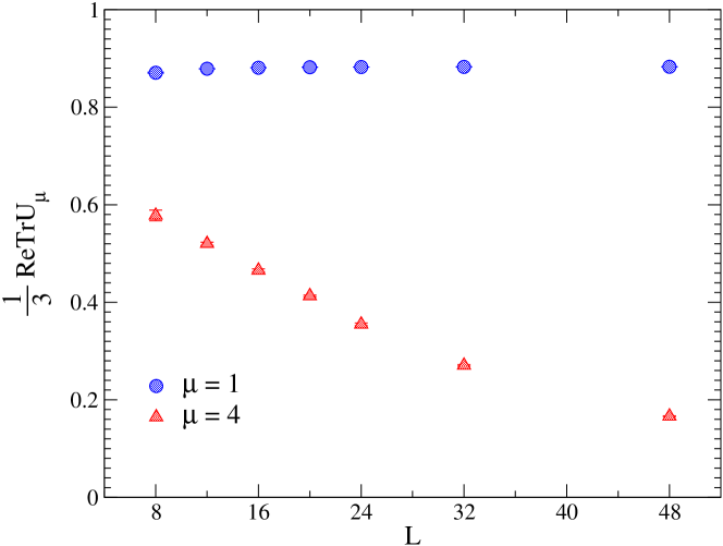
Figure 2: Mean link values $\langle\frac{1}{3}\operatorname{\mathfrak{Re}}\operatorname{Tr}U_{\mu}\rangle$ for different directions $\mu$ at $\beta=6.0$ as function of the linear lattice size $L$. Notice the strong volume dependence of $\langle\frac{1}{3}\operatorname{\mathfrak{Re}}\operatorname{Tr}U_{4}\rangle$ after residual gauge-fixing (RGF).

After having fixed the Coulomb gauge by maximizing the functional $F_{U}[g]$ there is still freedom to carry out gauge transformations $h_{t}\in SU(3)$ which only depend on time. One way to fix this residual gauge freedom is to maximize the functional

$$\widetilde{F}_{U}[h]=\sum_{t}\frac{1}{3}\operatorname{\mathfrak{Re}}\operatorname{Tr}\left\{h(t)\left[\sum_{\vec{x}}U_{4}(\vec{x},t)\right]h^{\dagger}(t+1)\right\}$$ (5)

where $U$ is the Coulomb-gauge transformed configuration (Eqs. 4). Links in time direction are finally gauge-transformed under $h(t)$ as

$$U_{4}(\vec{x},t)\to h(t)U_{4}(\vec{x},t)h^{\dagger}(t+1)$$ (6a)

whereas spatial links are transformed as

$$U_{i}(\vec{x},t)\to h(t)U_{i}(\vec{x},t)h^{\dagger}(t)\,,$$ (6b)

which preserves the Coulomb gauge. Equal-time observables involving only spatial links, i.e., the transversal gluon or the ghost propagator, are not affected by this residual gauge freedom.

If the transversal or the time-time gluon propagator was to be defined for non-equal time, the residual gauge would have to be fixed as well. For equal times, however, it is not clear to what extent, if at all, the results for the instantaneous time-time gluon propagator $D_{44}^{ab}(\vec{x})$ would change if the remaining gauge freedom was fixed. We will check this in Sect. VI by comparing data for $D_{44}$ for fixed residual gauge freedom (Berlin data) to that where this freedom was left unfixed (Osaka data).

In Fig. 1 we show the average trace $\langle\frac{1}{3}\operatorname{\mathfrak{Re}}\operatorname{Tr}U_{j}\rangle$ for spatial links after Coulomb gauge fixing (invariant under residual gauge fixing) and also the average $\langle\frac{1}{3}\operatorname{\mathfrak{Re}}\operatorname{Tr}U_{4}\rangle$ before and after residual gauge fixing as function of $\beta$. The data is taken for a $18^{4}$ lattice. Without residual gauge-fixing the average trace of time-like links vanishes, whereas after residual gauge-fixing the expectation value is finite and increases with increasing $\beta$. Fig. 2 demonstrates that the average $\langle\frac{1}{3}\operatorname{\mathfrak{Re}}\operatorname{Tr}U_{4}\rangle$ after residual gauge-fixing (shown for $\beta=6.0$) steeply decreases with increasing lattice volume, in contrast to $\langle\frac{1}{3}\operatorname{\mathfrak{Re}}\operatorname{Tr}U_{j}\rangle$ for spatial links.

In Sect. VI we will demonstrate that the difference of $D_{44}$ measured with and without residual gauge-fixing can be completely accounted for by a multiplicative, momentum-independent rescaling, e.g., by normalizing the matched $D_{44}$ propagator from both versions at some reference scale $p=\mu$. Apart from this, the residual gauge fixing has an impact only on the value of the propagator at zero momentum but this is not of importance for our present study.

III Coulomb-gauge propagators on the lattice

The space and time components of the gluon field evaluated in momentum space enter the bare instantaneous transversal and time-time gluon propagator as the Monte Carlo correlators

$$D^{ab}_{ij}(\vec{k}) =\left\langle\tilde{A}^{a}_{i}({\vec{k}})\tilde{A}^{b}_{j}({-\vec{k}})\right\rangle\,,$$ (7a)

$$D^{ab}_{44}(\vec{k}) =\left\langle\tilde{A}^{a}_{4}({\vec{k}})\tilde{A}^{b}_{4}({-\vec{k}})\right\rangle\,.$$ (7b)

Here $\tilde{A}_{i}$ and $\tilde{A}_{4}$ denote the spatial Fourier transforms of the lattice gluon fields at a fixed time $t$ with integer momenta $k_{i}\in\left(-L/2,L/2\right]$. An average over all time slices is understood. $D^{ab}_{ij}$ is diagonal in color space and transverse in momentum space. On the lattice it takes the form

$$D^{ab}_{ij}(\vec{k})=\delta^{ab}\left(\delta_{ij}-\frac{p_{i}(\vec{k})p_{j}(\vec{k})}{p^{2}}\right)D_{\rm tr}(p)$$ (8)

with

$$p_{i}(\vec{k})\equiv\frac{2}{a}\sin\left(\frac{\pi k_{i}}{L}\right)\,.$$ (9)

This is simply due to the lattice Coulomb gauge condition which in momentum space translates into

$$\sum_{i=1}^{3}p_{i}(\vec{k})\tilde{A}_{i}(\vec{k})=0\,$$ (10)

for all ${\vec{k}}$. In the following we use $p\equiv\big{\lvert}\,\vec{p}(\vec{k})\,\big{\rvert}$ to simplify the notation wherever applicable.

When analyzing data on $D^{ab}_{ij}$ it is natural to associate the physical momentum with $p$. Lattice results then reproduce the continuum tensor structure of $D^{ab}_{ij}$. Deviations from its tree-level form are described by the dimensionless dressing function $Z_{\mathrm{tr}}(p)$, defined by

$$Z_{\mathrm{tr}}=p\,D_{\mathrm{tr}}(p)\,.$$ (11)

Analogously, the time-time gluon propagator $D^{ab}_{44}$ may be presented in the form of either $D_{44}(p)$ or $Z_{44}(p)$. Both are related to the full propagator through

$$D^{ab}_{44}(\vec{k})=\delta^{ab}\,D_{44}(p)=\delta^{ab}\frac{Z_{44}(p)}{p}\,.$$ (12)

Depending on the particular focus, data below is presented in either one or the other form.

The ghost propagator is defined as the expectation value of the inverse Faddeev-Popov (FP) operator $M$

$$\left\langle\left(M^{-1}\right)^{ab}_{xx^{\prime}}\right\rangle=\delta_{tt^{\prime}}\delta^{ab}G(\vec{x}-\vec{x}^{\prime})$$ (13)

at a fixed time $t=t^{\prime}$ (subsequently averaged over all time-slices). The FP operator is local in time and, by virtue of the chosen Coulomb gauge functional (1), has on the lattice the dimensionless form

$$M^{ab}_{xx^{\prime}}=\delta_{tt^{\prime}}\sum_{i=1}^{3}\operatorname{\mathfrak{Re}}\operatorname{Tr}\Big{[}\left\{T^{a}\!,T^{b}\right\} \left(U_{i}(\vec{x},t)+U_{i}(\vec{x}-\hat{i},t)\right)\delta_{\vec{x}\vec{x}^{\prime}}$$

$$-2\,T^{b}T^{a}\,U_{i}(\vec{x},t)\,\delta_{\vec{x}+\hat{i},\vec{x}^{\prime}}-2\,T^{a}T^{b}\,U_{i}(\vec{x}-\hat{i},t)\,\delta_{\vec{x}-\hat{i},\vec{x}^{\prime}}\Big{]}$$ (14)

where $\hat{i}$ is a unit vector in spatial direction, $x\equiv(\vec{x},t)$ and $T^{a}$ is a generator of $SU(3)$ in the fundamental representation.

We are particularly interested in the momentum dependence of the ghost dressing function

$$J(p^{2})=\left({\vec{p}}({\vec{k}})\right)^{2}~{}G({\vec{p}}({\vec{k}}))\,,$$ (15)

where

$$G(\vec{p}({\vec{k}}))=\frac{a^{2}}{8L^{3}}\sum_{c,\vec{x},\vec{y}}e^{2\pi i\vec{k}\cdot(\vec{x}-\vec{y})/L}\left\langle\left(M^{-1}\right)^{cc}_{\vec{x},t;\vec{y},t}\right\rangle\,.$$ (16)

Working in momentum space, it is convenient to invert $M$ for a selection of momenta and colors $c$ forming right-hand side plane-wave sources $\xi^{c}(k)=\delta^{ac}e^{2\pi ik\cdot x/L}$ with $k=(\vec{k},0)\neq 0$. We use a preconditioned conjugate-gradient algorithm described in Ref. Sternbeck et al. (2005), adapted to Coulomb gauge, to accelerate the inversion of $M$. Alternatively, we could have used a selection of point sources $\xi$ and Fourier-transformed the vectors $[M^{-1}\xi](x)$ providing an estimator for the ghost propagator at once for all momenta, however with less statistical accuracy. The plane-wave method automatically ensures that $J(p^{2})$ is averaged over all time slices. Moreover, translational invariance is exploited to improve the estimator. Note that $M$ cannot be inverted for $\vec{k}=0$ due to its eight trivial (constant) zero eigenmodes.

Multiplicative renormalizability is a well-established property of the gluon and ghost propagators in Landau gauge. In Coulomb gauge, to our knowledge, this has been proven yet only up to one-loop by Watson and Reinhardt quite recently Watson and Reinhardt (2008). Their result for the bare dressing functions obtained in the 4D momentum space, formally translated from dimensional to lattice regularization looks as follows (omitting possible lattice corrections)

$$Z^{L}_{\mathrm{tr}} =1+g_{0}^{2}\,C_{\mathrm{tr}}\left[\log\left(a^{2}(x+y)\right)+H_{\mathrm{tr}}(\zeta)\right]+O(g_{0}^{4}),$$

$$Z^{L}_{44} =1+g_{0}^{2}\,C_{44}\left[\log\left(a^{2}(x+y)\right)+H_{44}(\zeta)\right]+O(g_{0}^{4}),$$

$$J^{L} =1+g_{0}^{2}\,C_{J}\left[\log(a^{2}y)+H_{J}\right]+O(g_{0}^{4}),$$ (17)

where the momentum variables are $x=p_{4}^{\,2},y=\vec{p}^{\,2},\zeta=x/y$, and the lattice cutoff is $a^{-1}$. $C_{\mathrm{tr}},C_{44},C_{J}$ and $H_{J}$ denote constants. Note the non-trivial dependence on $\zeta$ for both the Coulomb-gauge gluon dressing functions. When multiplicatively renormalizing the dressing functions, e.g., in a momentum subtraction (MOM) scheme at some scale $\mu$, this dependence has to be carefully taken into account (see also Burgio et al. (2008)), in particular for equal-time correlators which according to Eq. (17) require an integration over $p_{4}$ or $\zeta$. Of course, $a^{-1}\gg\mu$ has to be ensured for that which, admittedly, is very difficult to achieve in nowadays lattice computations. Even more, lattice computations are typically carried out at several values of $\beta$, i.e., at different cutoff-values. In general one should expect, that the corresponding dressing functions at different lattice spacings, say $a$ and $\overline{a}$, are related to each other by a finite renormalization of the $Z$-factors which will obviously depend only on the ratio $\overline{a}/a$ and not on the momenta. This will then hold also for the dressing functions Eq. (17) and correspondingly also for the equal-time correlators.

In the case of Landau gauge those $Z$-factors turned out to be close to unity for the gluon and ghost dressing functions at similar values of $\beta$. Therefore, it is more or less sufficient for them to express the various lattice spacings by a unique physical scale, e.g., via the Sommer-scale parameter $r_{0}=0.5~{}\text{fm}$ and the interpolation formula of Necco and Sommer Necco and Sommer (2002)

$$\ln(a/r_{0}) =-1.6804-1.7331(\beta-6.0)$$

$$+0.7849(\beta-6.0)^{2}-0.4428(\beta-6.0)^{3}$$ (18)

obtained from the lattice analysis of the static quark-antiquark potential and applicable in the range $5.7\leq\beta\leq 6.92$. The remaining lattice artifacts were sufficiently dealt with by applying cone and cylinder cuts to the momenta Leinweber et al. (1999). While a cone cut addresses finite-volume effects, the cylinder cut is an easy and effective method to reduce artifacts due to the broken rotational symmetry. We shall apply both these cuts also to our data shown below. However, in what follows we will demonstrate that the approach, even if sufficient for Landau gauge, is not quite enough for the case of Coulomb gauge. In fact, beside applying the usual cone and cylinder cuts one has to restrict momentum components to also satisfy $ap_{i}\leq\alpha<2$ and to apply non-trivial finite renormalizations between the different cutoff values.

Also, we shall not use a priori the Necco-Sommer scaling relation [Eq. (18)] but instead find the specific scaling behavior for each of the propagators defined above and present their data in terms of the finest available lattice scale at either $\beta=6.20$ or $6.10$. For this we employ the matching procedure of Ref. Leinweber et al. (1999) adapted here to Coulomb gauge. A detailed outline of this method applied to our propagators is given in Appendix A.

IV Discretization errors of the bare lattice data

We start our discussion by revisiting the strong scaling violations we reported for the transversal and the time-time gluon propagator in Nakagawa et al. (2007a); Voigt et al. (2007). There, we used the interpolation formula Eq. (18) to assign physical units to the lattice momenta and applied a multiplicative normalization at $\mu=2\mathrm{~{}GeV}$ for all values of $\beta$. This procedure, however, leads to serious disretization errors for both the instantaneous transversal and the time-time gluon propagator (see Fig. 3), whereas the ghost propagator looks much more satisfactory in this respect (see Fig. 4).

    

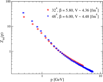
Figure 3: The instantaneous transverse gluon propagator (left) and the dressing function of the instantaneous time-time gluon propagator (right) using the Necco-Sommer scaling relation and normalized at $\mu=2~{}\textrm{GeV}$. The data refers to approximately equal physical volumes and has been cylinder and cone cut. Data was produced at HU Berlin.

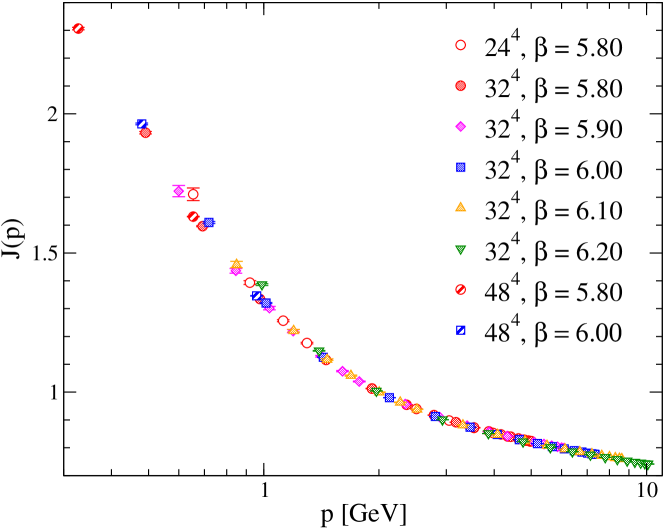
Figure 4: The ghost dressing function using the Necco-Sommer scaling relation and normalized at $\mu=2\mathrm{~{}GeV}$. The data has been cylinder and cone cut. Data at $\beta=5.8,6.0,6.2$ was collected at HU Berlin, data at $\beta=5.9,6.1$ at RCNP Osaka.

Challenged by these scaling violations, in the next sections we shall perform a matching procedure that merges the data for different $\beta$ into one bare lattice propagator associated with the highest available lattice cutoff.

    
    

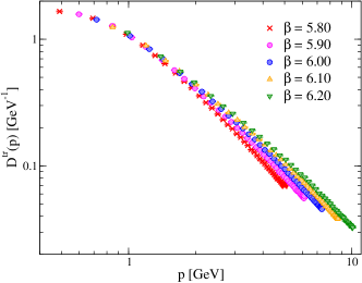
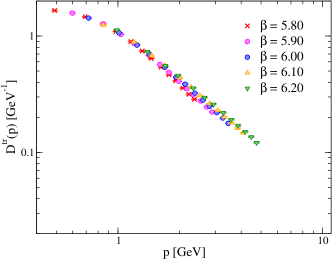
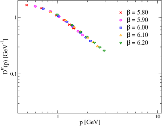
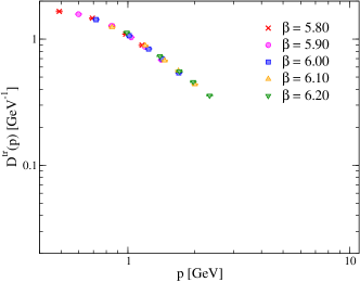
Figure 5: Effect of the $\alpha$-cut on the bare lattice data of the instantaneous transverse gluon propagator. The data (all for a $32^{4}$ lattice) is presented imposing different $\alpha$-cuts: no $\alpha$-cut (top left), $\lvert p_{i}a\rvert\leq 1$ (top right), $\lvert p_{i}a\rvert\leq 0.6$ (bottom left), $\lvert p_{i}a\rvert\leq 0.5$ (bottom right). Cylinder and cone cuts have been applied as before. Necco-Sommer scaling (with $r_{0}=0.5~{}\textrm{fm}$) has been used to get $a(\beta)$ and physical momenta $p$. The data for $\beta=5.8$, 6.0, 6.2 (5.9, 6.1) was obtained at HU Berlin (RCNP Osaka).

In a first step, however, we consider here the scaling violations and argue them to indicate that the admissible range of lattice momenta needs to be restricted even further than what the cylinder and cone cuts would do. For this, we introduce a new momentum cut that will be applied in addition to those two cuts. Basically, not the full Brillouin zone should be eligible when analyzing the corresponding propagator data, but only that at momenta (Eq. (9)) whose components are restricted to $\lvert p_{i}a\rvert\leq\alpha<2$. For the sake of brevity we will refer to this cut as the “$\alpha$-cut” in what follows.

Fig. 5 illustrates the effect of the $\alpha$-cut on the instantaneous transversal gluon propagator. Note that in this figure (as in Nakagawa et al. (2007a); Voigt et al. (2007)) we have used the Necco-Sommer formula (18) (and $r_{0}=0.5~{}\textrm{fm}$) to assign physical units to momenta and propagator. Obviously, when decreasing $\alpha$ less and less data points survive this cut but those that do show a much better overlap than before (see, in particular, the lower panels of Fig. 5).

V Matching the transversal gluon propagator

Still, the disagreement between data from different $\beta$ does not completely disappear. Therefore, in a next step, we relax the a priori universal $a(\beta)$ dependence (e.g., that according to Eq. (18)) and apply the matching procedure of Ref. Leinweber et al. (1999) as explained in Appendix A. It provides us with multiplicative renormalization factors depending on the ratios of the lattice spacings and with the specific dependence of the lattice spacing $a=a(\beta)$ separately for each propagator.

We start with the instantaneous transversal gluon propagator and first match data obtained on two lattices with approximately the same physical volume, i.e., data on a $L^{4}=32^{4}$, $\beta=5.8$ lattice with data on a $L^{4}=48^{4}$, $\beta=6.0$ lattice. Besides the cone and cylinder cuts we apply two different $\alpha$-cuts (with $\alpha=0.6$ and $\alpha=0.5$) before performing the matching procedure. Our aim is to compare the influence of the $\alpha$-cut on the quality of matching. The result, with $L^{4}=32^{4}$, $\beta=5.8$ being the coarse and $L^{4}=48^{4}$, $\beta=6.0$ being the fine lattice, is shown in Fig. 6 for both $\alpha$-cuts.

    

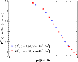
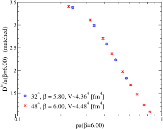
Figure 6: The instantaneous transverse gluon propagator obtained by matching data from two lattices with approximately equal physical volume. Besides cylinder and cone cuts, an $\alpha$-cut has been imposed with $\alpha=\lvert p_{i}a\rvert\leq 0.6$ (left) and $\alpha=\lvert p_{i}a\rvert\leq 0.5$ (right). Data collected at HU Berlin.

We obtain good matching of both data sets with a better result for $\alpha=0.5$ (see the $\chi^{2}/dof$ listed in Table 2). There is hardly any difference between the best result of the matching procedure on one hand and directly imposing the Necco-Sommer scaling relation on the other (Fig. 5). Indeed, our matching procedure nearly reproduces the lattice-spacing ratios as given through Eq. (18) (see Table 2) in Appendix B.

Next we extend the matching to all values of $\beta=5.8\ldots 6.2$ using data obtained on $32^{4}$ and $48^{4}$ lattices. Since $\beta=6.2$ has the finest lattice spacing, the matching is performed between data at $\beta=6.2$ (setting the reference scale) and data at all other $\beta=5.8\ldots 6.1$. We also compare the result for four different $\alpha$-cuts. The results are summarized in Table 3.

We not only find the ratios of lattice spacings to rise monotonously upon decreasing $\beta$, but also the ratios of the renormalization constants to be about the same (somewhat below $1.0$), i.e., almost independent on $\beta$.

As a general rule, smaller values for $\alpha$ result in lower $\chi^{2}/dof$ values and hence better matching. We also see that the matching procedure nearly always results in a lattice-spacing ratio smaller than that given through Eq. (18), although the discrepance decreases with $\alpha$ taken smaller. As shown in Fig. 7 for the best $\alpha$-cut ($\alpha=0.5$), we achieve a virtually perfect matching of the instantaneous transversal gluon propagator over all data obtained at $\beta=5.8\ldots 6.2$. Comparing with the $\chi^{2}/dof$ for $\alpha=1.0$, we conclude that applying the $\alpha$-cut is essential to achieve a good overlap of the data. Our combined final result indicates a flattening of the propagator in the infrared region which is worth to be explored further. We expect a tendency to show a plateau as recently seen in the Landau gauge case Bogolubsky et al. (2009), which excludes a vanishing gluon propagator in the infrared limit.

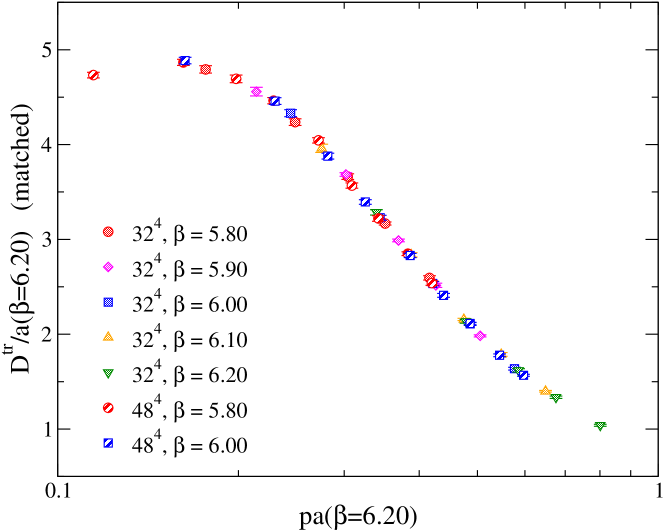
Figure 7: The instantaneous transverse gluon propagator obtained by matching all data from $32^{4}$ and $48^{4}$ lattices, including data from both Osaka and Berlin collected at five different $\beta$ values. The result is shown for a fixed $\alpha$-cut with $\lvert p_{i}a\rvert\leq 0.5$. Data are cylinder and cone cut.

VI Matching the time-time gluon propagator

  

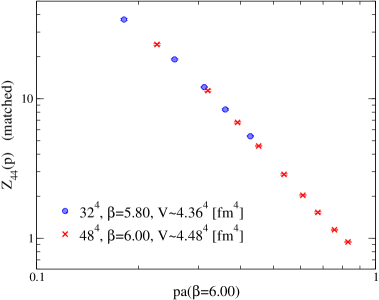
Figure 8: The instantaneous time-time gluon dressing function after matching Berlin data from two lattices of approximately equal physical volume and applying cylinder and cone cuts. Two $\alpha$-cuts are compared: $\lvert p_{i}a\rvert\leq 0.6$ (left) and $\lvert p_{i}a\rvert\leq 0.5$ (right).

We now apply the matching procedure to the instantaneous time-time gluon propagator $D_{44}$. As for the transversal propagator $D_{tr}$, we first match data obtained on two lattices with approximately the same physical volume, i.e., data for $L^{4}=32^{4}$, $\beta=5.8$ with data for $L^{4}=48^{4}$ and $\beta=6.0$, respectively. We also compare the effect of two different $\alpha$-cuts ($\alpha=0.6$ and $\alpha=0.5$) in addition to the usual cylinder and cone cuts.

Whereas the matching seems to work reliably as shown in Fig. 8 and as demonstrated in Table 4 by the low $\chi^{2}/dof$ value for $\alpha=0.5$, the obtained lattice spacing ratio is now significantly larger than predicted by the Necco-Sommer scaling relation (see Table 4). This is in striking contrast to what we have observed in the case of the transversal gluon propagator.

We now merge all data for $D_{44}$ in the interval $\beta=5.8\ldots 6.2$ obtained on $32^{4}$ and $48^{4}$ lattices. However, since the instantaneous time-time gluon propagator is more sensitive to Gribov copies Voigt et al. (2007) and since we have employed different gauge fixing procedures at HU Berlin and at RNCP Osaka, we first match the corresponding data sets separately. The resulting fit parameters are summarized in Table 5 (Osaka) and Table 6 (Berlin).

Matching the Osaka data one finds that the ratios $R_{a}$ of lattice spacings rise monotonously upon decreasing $\beta$ but much stronger than in Eq. (18). The ratio of renormalization constants is still compatible with unity for $\beta=6.0$ if compared to $\beta=6.1$ (providing the reference scale), but it decreases abruptly between $\beta=6.0$ and $\beta=5.9$. The $\chi^{2}/dof$ value is acceptable only for an $\alpha$-cut where $\alpha=0.5$.

The Berlin data allows only to compare $\beta=6.0$ and $\beta=5.8$ to $\beta=6.2$ (which sets the reference scale). The ratios of the lattice spacings are compatible with the results for the Osaka data. The ratio of the renormalization constants is still compatible with unity for $\beta=6.0$, if compared to $\beta=6.2$, but drops between $\beta=6.0$ and $\beta=5.8$ similar to the Osaka data. The $\chi^{2}/dof$ is unacceptably large.

In Fig. 9 we show our final result for the instantaneous time-time gluon propagator having matched and combined all the Osaka and Berlin data. We have now used a unique scale set by $a(\beta=6.0)$ to give all momenta in physical units. The quality of the fits in this case is worse compared with the fits of the transverse gluon propagator. Nevertheless, the scaling behavior does look quite reasonable and there is an improvement compared to the results presented in Table 4. The reason is probably that we have moved closer to the continuum limit by including data from $\beta=6.1$ and $\beta=6.2$. In the infrared region the data points obtained in Berlin and Osaka split. We interprete this as a consequence of the use of different gauge fixing techniques. The more efficient simulated annealing method weakens the singular behavior as seen also for the ghost propagator Voigt et al. (2008).

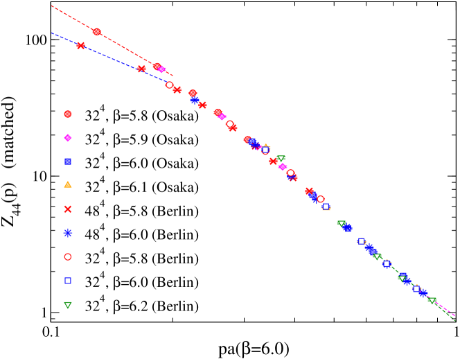
Figure 9: The dressing function of the instantaneous time-time gluon propagator after matching Berlin and Osaka data separately on $32^{4}$ and $48^{4}$ lattices for five different $\beta$ values. Fit parameters underlying the matching are listed in Tabs. 5 and 6. Data has been cylinder and cone cut and results are shown for a fixed $\alpha$-cut with $|p_{i}a|\leq 0.5$. The two fits for the momentum dependence in the IR are described in Sect. IX.

In passing, we revisit the question whether there is a difference between the instantaneous time-time gluon propagator if one is applying the residual gauge-fixing (Berlin data) or not (Osaka data). Fig. 10 shows the results for $\beta=6.0$. The propagator at momentum $pa\neq 0$ seems not to depend on the volume, but on the procedure (cf. the left panel). The latter is understandable if one looks back at Fig. 1 and there at the difference for the time-like links. It is remarkable that the difference between the two cases can be eliminated by a uniform multiplicative rescaling. This is accomplished by normalizing the propagator $D_{44}/a$ at $pa=2.0$ to 1.0 (cf. the right panel). The residual gauge fixing has only an impact on the value of the propagator at zero momentum, $D_{44}(ap=0)/a$. With residual gauge fixing this value is obviously smaller as expected.

    

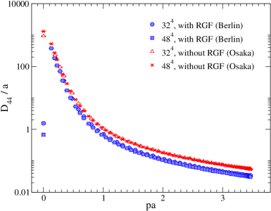
Figure 10: Left: comparison between the unrenormalized instantaneous time-time gluon propagator $D_{44}$ with and without the residual gauge fixing. Right: the same but formally normalized at $pa=2$. The cylinder cut has applied. Berlin and Osaka data for $\beta=6.0$ and lattice sizes $32^{4}$ and $48^{4}$ are shown together.

VII Matching the ghost propagator

Finally we apply the matching procedure to the ghost propagator. As we have seen in Fig. 4, Necco-Sommer scaling is only weakly violated. Therefore, we expect a matching result that closely follows this behavior.

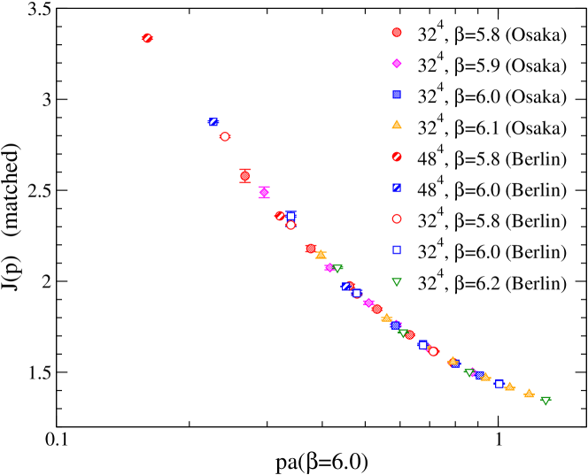
Figure 11: The ghost dressing function after matching data from $32^{4}$ and $48^{4}$ lattices including data from both Osaka and Berlin at five different $\beta$ values. For the fits see Table 7 and Table 8. The result is shown for a fixed $\alpha$-cut: $\lvert p_{i}a\rvert\leq 0.5$. Both the cylinder and the cone cut are applied as usual.

The fitting results (respectively for the Osaka and Berlin data) are presented in Tabs. 7 and 8, there relative to the highest $\beta_{\rm max}=6.1$ and $\beta_{\rm max}=6.2$ in both cases. For no $\alpha$-cut ($\alpha=2.0$) the ratios of lattice spacing $a(\beta)/a(\beta_{\rm max})$ reproduce almost perfectly the corresponding ratios according to Eq. (18). Nevertheless, we notice that a smaller $\alpha$ leads to some deviation from that scaling, in particular at the lowest $\beta$. Including the results of the separate fits, the Osaka and Berlin data are afterwards combined in Fig. 11 showing there the result only for the most restrictive $\alpha$-cut ($\alpha=0.5$).

Matching the Osaka data yields an overall very good $\chi^{2}/dof$. The ratios of the renormalization constants are all compatible with unity, and the ratios of lattice spacings rise monotonously upon decreasing $\beta$. When no $\alpha$-cut is applied the fitted $R_{a}$ rise in accordance with Eq. (18), while restricted $\alpha$-cuts lead to $R_{a}$’s which grow slightly slower. Matching the Berlin data results in the same tendencies, but the $\chi^{2}/dof$ turned out to be very large. Probably due to the fact that the Berlin ghost data are averaged over all time slices and the Osaka data are not, the errors of the Berlin data are smaller by an order of magnitude.

VIII The scaling behavior of the propagators

  

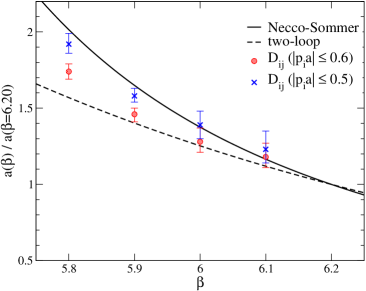
Figure 12: The scaling relation as it emerges from matching the data obtained in simulations with the Wilson action. Left: for the transversal gluon propagator with two $\alpha$-cuts for comparison. Right: for the ghost propagator with no $\alpha$-cut ($\alpha=2.0$) and an $\alpha$-cut with $\alpha=0.6$ for comparison, and for the time-time gluon propagator with an $\alpha$-cut with $\alpha=0.6$, a rather conservative momentum cut.

At this point we can check now if our individual results on $a(\beta)$ reproduce a unique running lattice scale. We had started with Necco-Sommer scaling, but abandoned this, fully relying on the matching procedure to produce the “correct” lattice scale function. Let us remind that the lattice scales as found may deviate from asymptotic scaling (which of course is strictly valid only for $\beta\to\infty$) and also from that derived for other observables (e.g., Necco-Sommer scaling derived for the static quark-antiquark force in pure $SU(3)$ gauge theory).

With Fig. 12 we summarize our results on the fitted scaling behavior of the lattice spacing in terms of the finest lattice spacing available in our study. For all the propagators considered we have plotted the ratios of the lattice spacings relative to the finest lattice (at $\beta=6.2$ for the transverse gluon propagator in the left panel, and at $\beta=6.1$ for $D_{44}$ and the ghost propagators in the right panel, respectively) as a function of $\beta$ as found through the matching procedure with two choices of the $\alpha$-cut. For the transversal gluon propagator the data points (corresponding to both choices of $\alpha$-cuts) fit very well between the curves corresponding to two-loop running of the lattice spacing,

$$a=\frac{1}{\Lambda_{\textrm{Lat}}}\left(\frac{8\pi^{2}}{11N_{c}}\beta\right)^{\frac{51}{121}}\exp\left(-\frac{4\pi^{2}}{11N_{c}}\beta\right)\,.$$ (19)

and to the relation (Eq. (18)). The same is observed for the ghost propagator. In this case, also applying no cut ($\alpha=2.0$) results in a reasonable result.

On the other hand, the $a(\beta)$ dependence as found from the matching procedure of the instantaneous time-time gluon propagator is not only much stronger than in Eq. (18), but also inconsistent with the scaling law for the other propagators. We cannot say to which extent such a faster running is beyond some general bound and unfortunately have to conclude that the problem of the bad scaling behavior for the instantaneous time-time gluon propagator remains unsolved yet.

IX Fitting the behavior at large and small momentum

Having successfully merged data for the propagators from simulations at different $\beta$ values, one may try to fit their ultraviolet (UV) behavior and partly also to extract some infrared (IR) exponents.

For the transverse gluon propagator we try a power-law ansatz

$$D^{\rm tr}(\lvert\vec{p}\rvert)^{\mathrm{UV}}=\frac{1}{|\vec{p}|}\left(\frac{c_{\rm tr}}{|\vec{p}|}\right)^{\eta_{\rm tr}},$$ (20)

to describe the behavior at large momenta. For the UV fitting we use the data points above some minimal momentum ($\lvert\vec{p}\rvert_{\mathrm{min}}$ in units of $a^{-1}(\beta=6.2)$) and investigate the dependence of the anomalous dimension $\eta_{\rm tr}$ on the fitting range and the $\alpha$-cut. Fit results are collected in Table 9 and our best fits (with $\alpha=0.5$) give $\eta_{\rm tr}=0.40(2)$. Qualitatively, the behavior we find is similar to the UV fit given in Ref. Langfeld and Moyaerts (2004), though there [for $SU(2)$] a somewhat bigger exponent $\eta_{\rm tr}=0.5(1)$ was found.

For the longitudinal gluon dressing function $Z_{44}$ we try power law ansatzes both in the UV and in the IR regions

$$Z_{44}(|\vec{p}|)^{\mathrm{UV}}=\left(\frac{c_{44}}{|\vec{p}|}\right)^{\eta_{44}}\,,~{}~{}~{}Z_{44}(|\vec{p}|)^{\mathrm{IR}}=\left(\frac{d_{44}}{|\vec{p}|}\right)^{\kappa_{44}}\,.$$ (21)

The results are collected in Tabs. 10 and 11, respectively. This dressing function was not studied in Ref. Langfeld and Moyaerts (2004).

For the ghost dressing function, analogous to Ref. Langfeld and Moyaerts (2004), we adopt a logarithmic ansatz in the UV region

$$J(|\vec{p}|)^{\mathrm{UV}}=\frac{c_{\rm gh}}{\ln(|\vec{p}|/\Lambda_{\textrm{Coul}})^{\gamma}}\,,$$ (22)

and a power-law ansatz for the IR behavior

$$J(|\vec{p}|)^{\mathrm{IR}}=\left(\frac{d_{\rm gh}}{|\vec{p}|}\right)^{\kappa_{\rm gh}}\,.$$ (23)

Fits results for either momentum region are given in Tabs. 12 and 13, respectively. The UV fits scatter with $\alpha$ (the additional momentum cut), though, the most stable results are obtained for no $\alpha$-cut ($\alpha=2.0$). With a suitably restricted fit interval fits are stable and give $\Lambda_{\rm Coul}a(\beta=6.0)=0.275(20)$ or $\Lambda_{\rm Coul}r_{0}=1.37(10)$ and $\gamma=0.33(1)$. For $SU(2)$ this exponent was found to be $\gamma=0.26(2)$ Langfeld and Moyaerts (2004).

The IR fits are quite stable and give $\kappa_{\rm gh}=0.435(6)$ without applying $\alpha$-cuts, even though we admit that the $\chi^{2}/dof$ values are rather large. In Ref. Langfeld and Moyaerts (2004) a value $\kappa_{\rm gh}=0.49(1)$ was found (corresponding to $2\kappa$ there).

X Conclusions

We have investigated the momentum dependence of the instantaneous ghost and gluon propagators of pure $SU(3)$ lattice Coulomb gauge theory. Our study represents a joint analysis of data from lattice simulations independently performed at Berlin and Osaka for the Wilson gauge action in the range $\beta=5.8,\ldots,6.2$.

For these values of $\beta$, we find apparent scaling violations for both the spatially transversal and the time-time gluon propagator, while for the ghost propagator such violations are surprisingly mild. Our inspection of the gluon propagator data shows that the violations there are basically due to data that survives a cylinder cut but involves momentum components close to the upper end of the Brillouin zone. Consequently, if additionally an $\alpha$-cut like $\lvert p_{i}a\rvert\leq 0.5$ is applied to the data, scaling violations are under much better control. The price to pay are strong restrictions of allowed momenta which, in our opinion, should not only satisfy the cylinder and cone cuts but also $\lvert p_{i}a\rvert\leq 0.5$ ($\alpha$-cut). This is the first result of our paper.

Second, we find that the scaling violations can be sufficiently reduced if, in addition to the aformentioned cuts, a matching procedure (see Appendix A) is used to merge data. That is, instead of imposing one particular $a(\beta)$ dependence (e.g., that of Ref. Necco and Sommer (2002)) and normalizing the data for the different lattice cutoffs such that they coincide at a particular reference scale, both the $a(\beta)$ dependence and the relative normalization factors are determined through an optimization method that seeks the best overlap of data. It turns out, that the matching procedure applied to either the transversal gluon or the ghost propagator provides us with a $a(\beta)$ dependence only slightly different from what is known from Necco and Sommer (2002), somewhere in between Necco-Sommer scaling and asymptotic two-loop scaling. Note that the matching procedure would allow us to fix the lattice spacing if we were to simulate also beyond the interval $5.7\leq\beta\leq 6.92$ covered by the Necco-Sommer analysis.

Generally we can say that the matching analysis results in ratios of the renormalization constants closer to unity at $\beta\geq 6.0$. Future lattice studies of gluon and ghost propagators should be performed in that region. The fact that – except for the ghost propagator – the matching performs better the more restrictive $\alpha$-cuts are applied shows that the momenta with components close to the upper end of the Brillouin zone are far from the continuum limit. This might signal a more general effect, namely that observables closer to the infrared region have better scaling properties.

Unfortunately, we could not correct the scaling violations for the instantaneous time-time gluon propagator. For this, these violations are so strong that the $a(\beta)$ dependence as found through the matching is far from what we find for the other propagators. In fact, $a(\beta)$ in this case is found running too fast. Moreover, for $\beta\leq 5.9$ the ratio of renormalization constants drops compared to the behavior at $\beta\geq 6.0$ such that the assumptions and results of the matching analysis for the $D_{44}$ propagator must be considered with caution.

We mention that for the $SU(2)$ transversal gluon propagator it has been argued Burgio et al. (2008) that the correct instantaneous propagator can be reconstructed only from the full 4-dimensional space-time propagator. There, a residual gauge-fixing was applied that enforces $A_{4}=\mathrm{const}$. Therefore, it needs to be scrutinized whether the scaling violations, that we have seen here for the transversal gluon propagator, are really due to the alleged (multiplicative) non-renormalizability of the Coulomb gauge Watson and Reinhardt (2007) when residual gauge-fixing is applied or not. Our results for the transversal propagator suggest a more mundane resolution: exclude too large momenta from the analysis and allow for an independently determined running lattice spacing, then data within a very restricted range of momenta (in units $a$) can be successfully merged and gives a $a(\beta)$ dependence that agrees with what is known form the literature.

We stress again that our result for the time-time gluon propagator is non-acceptable. The $a(\beta)$ dependence as found for this is far from the running scale for the other propagators. In the light of this, the argument of non-renormalizability might still be valid for the $A_{4}$ component of the gluon field.

When applying fits to the data at either low or large momenta (though restricted by quite stringent bounds) we obtain qualitatively similar UV and IR fits as reported for the $SU(2)$ theory in Langfeld and Moyaerts (2004).

Appendix A Matching procedure

    

Figure 13: Details of matching $Z^{\mathrm{tr}}$ measured on a $L^{4}=32^{4}$, $\beta=5.8$ lattice with the data obtained on a $L^{4}=48^{4}$, $\beta=6.0$ lattice. An $\alpha$-cut with $\lvert p_{i}a\rvert\leq 0.5$ was applied before matching. Left: $\chi^{2}/dof$ as a function of the ratio of lattice spacings $R_{a}=a_{c}(5.8)/a_{f}(6.0)$. Right: the 68.3% confidence region spanned by ratios of lattice spacing $R_{a}=a_{c}(5.8)/a_{f}(6.0)$ and renormalization constants $R_{Z}=Z(5.8)/Z(6.0)$ determined through the matching procedure.

In this appendix we describe the matching procedure of Leinweber et al. (1999) applied to Coulomb gauge. The procedure does not rely on any given lattice scale dependence $a(\beta)$ but allows us to extract this for each propagator individually.

Under the assumption that the fixed-time gluon and ghost propagators in Coulomb gauge can be renormalized multiplicatively (see Sect. III and Ref. Watson and Reinhardt (2008)), we aim at an optimal overlap of bare propagator data from a coarse lattice (with unknown lattice spacing $a_{c}$) and a fine lattice (with a lattice spacing $a_{f}$ that might be known). Using the fact that the bare and dimensionless lattice propagator $D^{L}$ is a function of the product of the three-momentum $p$ with the lattice spacing $a$ only (the dependence on $\beta$ is of course kept in mind), and assuming that multiplicative renormalization is valid, the bare propagators on the fine and coarse lattice are related by

$$a_{f}D^{L}_{f}(pa_{f})=R_{Z}(a_{f}/a_{c})~{}\cdot~{}a_{c}D^{L}_{c}(pa_{c})$$ (24)

The renormalization factor $R_{Z}$ only depends on the ratio of the lattice cutoffs $R_{a}=a_{f}/a_{c}$. Taking the logarithm gives

$$\ln D^{L}_{f}(pa_{f})=\ln D^{L}_{c}(pa_{c})-\ln R_{a}+\ln R_{Z}\,.$$ (25)

Expressing the momentum on the coarse lattice in terms of the momentum on the fine lattice by

$$a_{c}=\frac{a_{f}}{R_{a}}\quad\Longleftrightarrow\quad\ln(pa_{c})=\ln(pa_{f})-\ln R_{a}\,,$$ (26)

we arrive at

$$\ln D^{L}_{f}[\ln(pa_{f})] =\ln D^{L}_{c}[\ln(pa_{f})-\ln R_{a}]-\ln R_{a}+\ln R_{Z}$$

$$=\ln D^{L}_{c}[\ln(pa_{f})+\Delta_{a}]+\Delta_{Z}\,,$$ (27)

where $R_{a}=e^{-\Delta_{a}}$ and $R_{Z}=e^{-\Delta_{a}+\Delta_{Z}}$.

Notice that $\Delta_{a}$ and $\Delta_{Z}$ are positive. We find the values for $R_{a}$ and $R_{Z}$ from a fitting procedure as follows.

Suppose that we have one data set $\{x=pa_{f},D^{L}_{f},\sigma_{f}\}_{i}$ with $i=1,\ldots,n_{f}$ for the fine lattice and one data set $\{y=pa_{c},D^{L}_{c},\sigma_{c}\}_{j}$ with $j=1,\ldots,n_{c}$ for the coarse lattice with $\sigma$ denoting the statistical error of the propagator $D^{L}$, and $n_{f}$ resp. $n_{c}$ denoting the number of data points for the propagator on the fine and coarse lattice, respectively. Then, we use a $\chi^{2}$ fit to optimally match both data sets, i.e., to find the optimal overlap of the bare lattice propagator from the fine and the coarse lattice. To be specific, we minimize

$$\chi^{2}=\sum_{i=1}^{n_{f}}\left(\frac{D^{L}_{\textrm{f}}(x_{i})-\frac{R_{Z}}{R_{a}}D^{L~{}\textrm{int}}_{\textrm{c}}\left(\frac{x_{i}}{R_{a}}\right)}{\sigma_{\textrm{f},i}}\right)^{2}+\sum_{j=1}^{n_{c}}\left(\frac{D^{L}_{\textrm{c}}(y_{j})-\frac{R_{a}}{R_{Z}}D^{L~{}\textrm{int}}_{\textrm{f}}\left(y_{j}R_{a}\right)}{\sigma_{\textrm{c},j}}\right)^{2}\,.$$ (28)

In the first term $D^{L}_{\textrm{f}}$ is represented by the measured values at the momenta $p_{i}$ (expressed as function of $x_{i}=p_{i}a_{f}$) and the corresponding error $\sigma_{\textrm{f},i}$, while $D_{\textrm{c}}^{L~{}\textrm{int}}$ is evaluated at these momenta by a cubic spline interpolation of the data for $D_{\textrm{c}}^{L}$ . In the second term, the rôle of $D_{\textrm{f}}^{L}$ and $D_{\textrm{c}_{L}}$ is interchanged with respect to genuine data ($y_{j}=p_{j}a_{c}$ in $D_{\textrm{c}_{L}}$) and interpolation of $D_{\textrm{f}}^{L}$. With this definition of $\chi^{2}$ the matching is done as follows:

1. Vary $\Delta_{a}$ over an interval $(0,1]$ with step size $0.001$ and determine the optimal $\Delta_{Z}$ giving the lowest $\chi^{2}/dof$ for each value of $\Delta_{a}$ considered,

2. Identify the best overall combination of $\Delta_{a}$ and $\Delta_{Z}$ by searching for the global minimum of $\chi^{2}/dof$.

This provides us with the optimal choice of $R_{a}$ and $R_{Z}$. The error of $R_{a}$ and $R_{Z}$ are given by the 68.3% confidence region, i.e., the region of fit parameters $R_{a}$ and $R_{Z}$ with $\chi^{2}/dof<\chi^{2}_{\mathrm{min}}/dof+1$. An illustration of this is given in Fig. 13 for matching the instantaneous transversal gluon propagator measured on a $L^{4}=32^{4}$, $\beta=5.8$ lattice with data obtained on a $L^{4}=48^{4}$, $\beta=6.0$ lattice (cf. Sect. V, Fig. 6 and Table 2).

Note that applying this procedure to several combinations of fine and coarse lattices provides us with an optimal scaling relation $a=a(\beta)$ for each propagator.
 

Appendix B Tables

In this appendix we present an overview of the data sets produced in Osaka and Berlin, the results of all matching fits according to Secs. V, VI, VII and Appendix A as well as of the fits in the infrared (IR) and ultraviolet (UV) limits as described in Sect. IX.

Table 1: Lattice parameters used in this study. Configurations were generated at RCNP Osaka and HU Berlin.

$L^{4}$	$\beta$	$a^{-1}$ [GeV]	$a$ [fm]	$V$[fm4]	#conf	group
$12^{4}$	5.8	1.446	0.1364	1.644	100	Berlin
$16^{4}$	:	:	:	2.184	40	Berlin
$18^{4}$	:	:	:	2.464	80	Osaka
$24^{4}$	:	:	:	3.274	40	Osaka
$24^{4}$	:	:	:	3.274	30	Berlin
$32^{4}$	:	:	:	4.364	20	Osaka
$32^{4}$	:	:	:	4.364	30	Berlin
$48^{4}$	:	:	:	6.554	20	Berlin
$18^{4}$	5.9	1.767	0.1116	2.094	80	Osaka
$24^{4}$	:	:	:	2.784	40	Osaka
$32^{4}$	:	:	:	3.714	20	Osaka
$12^{4}$	6.0	2.118	0.0932	1.124	100	Berlin
$16^{4}$	:	:	:	1.494	60	Berlin
$18^{4}$	:	:	:	1.684	80	Osaka
$24^{4}$	:	:	:	2.244	40	Osaka
$24^{4}$	:	:	:	2.244	40	Berlin
$32^{4}$	:	:	:	2.984	20	Osaka
$32^{4}$	:	:	:	2.984	30	Berlin
$48^{4}$	:	:	:	4.484	20	Berlin
$18^{4}$	6.1	2.501	0.0788	1.424	80	Osaka
$24^{4}$	:	:	:	1.894	40	Osaka
$32^{4}$	:	:	:	2.524	20	Osaka
$12^{4}$	6.2	2.914	0.0677	0.814	100	Berlin
$16^{4}$	:	:	:	1.084	40	Berlin
$24^{4}$	:	:	:	1.624	30	Berlin
$32^{4}$	:	:	:	2.174	20	Berlin

Table 2: Fit parameters obtained upon matching $D^{\mathrm{tr}}$ data from a $(L^{4},\beta)=(32^{4},5.8)$ and a $(48^{4},6.0)$ lattice for two different $\alpha$-cuts (see Fig. 6). For comparison we also show the lattice spacing ratios according to Eq. (18).

$\lvert p_{i}a\rvert\leq\alpha$	$\frac{a(5.8)}{a(6.0)}$	$\frac{a^{\mathrm{NS}}(5.8)}{a^{\mathrm{NS}}(6.0)}$	$R_{Z}\left(\frac{a(5.8)}{a(6.0)}\right)$	$\chi^{2}/dof$
$\alpha=0.6$	$1.37^{+3}_{-4}$	$1.46$	$0.989^{+10}_{-10}$	$3.28$
$\alpha=0.5$	$1.41^{+4}_{-5}$	$1.46$	$0.998^{+11}_{-11}$	$0.92$

Table 3: Matching the transversal gluon propagator for five $\beta$ values (see Fig. 7): shown are the ratios of lattice spacings relative to the finest one obtained either by the matching procedure or according to Eq. (18); the ratios of the renormalization constants and the corresponding $\chi^{2}/dof$ of the fit that accomplishes the matching, for four choices of the $\alpha$-cut. The lattice size is $32^{4}$.

$|p_{i}a|\leq\alpha$	$\beta$	$\frac{a(\beta)}{a(6.2)}$	$\frac{a^{\mathrm{NS}}(\beta)}{a^{\mathrm{NS}}(6.2)}$	$R_{Z}(\frac{a(\beta)}{a(6.2)})$	$\chi^{2}/dof$
$\alpha=1.0$	$5.8$	$1.51^{+4}_{-4}$	$2.01$	$0.982^{+12}_{-13}$	$5.56$
	$5.9$	$1.31^{+5}_{-5}$	$1.65$	$0.990^{+19}_{-18}$	$3.83$
	$6.0$	$1.19^{+7}_{-7}$	$1.38$	$0.993^{+34}_{-26}$	$2.39$
	$6.1$	$1.12^{+10}_{-20}$	$1.17$	$0.984^{+108}_{-36}$	$6.30$
$\alpha=0.8$	$5.8$	$1.68^{+4}_{-6}$	$2.01$	$0.961^{+12}_{-10}$	$2.16$
	$5.9$	$1.43^{+5}_{-6}$	$1.65$	$0.970^{+16}_{-15}$	$2.98$
	$6.0$

References

- Mandula and Ogilvie (1987) J. E. Mandula and M. Ogilvie, Phys. Lett. B185, 127 (1987).
- Marenzoni et al. (1995) P. Marenzoni, G. Martinelli, and N. Stella, Nucl. Phys. B455, 339 (1995), eprint hep-lat/9410011.
- Suman and Schilling (1996) H. Suman and K. Schilling, Phys. Lett. B373, 314 (1996), eprint hep-lat/9512003.
- Nakamura et al. (1995) A. Nakamura, H. Aiso, M. Fukuda, T. Iwamiya, T. Nakamura, and M. Yoshida (1995), eprint hep-lat/9506024.
- Leinweber et al. (1998) D. B. Leinweber, J. I. Skullerud, A. G. Williams, and C. Parrinello (UKQCD), Phys. Rev. D58, 031501 (1998), eprint hep-lat/9803015.
- Becirevic et al. (1999) D. Becirevic et al., Phys. Rev. D60, 094509 (1999), eprint hep-ph/9903364.
- Mandula (1999) J. E. Mandula, Phys. Rept. 315, 273 (1999), eprint hep-lat/9907020.
- von Smekal et al. (1997) L. von Smekal, R. Alkofer, and A. Hauck, Phys. Rev. Lett. 79, 3591 (1997), eprint hep-ph/9705242.
- von Smekal et al. (1998) L. von Smekal, A. Hauck, and R. Alkofer, Ann. Phys. 267, 1 (1998), eprint hep-ph/9707327.
- Bonnet et al. (2000) F. D. R. Bonnet, P. O. Bowman, D. B. Leinweber, and A. G. Williams, Phys. Rev. D62, 051501 (2000), eprint hep-lat/0002020.
- Bonnet et al. (2001) F. D. R. Bonnet, P. O. Bowman, D. B. Leinweber, A. G. Williams, and J. M. Zanotti, Phys. Rev. D64, 034501 (2001), eprint hep-lat/0101013.
- Bowman et al. (2004) P. O. Bowman, U. M. Heller, D. B. Leinweber, M. B. Parappilly, and A. G. Williams, Phys. Rev. D70, 034509 (2004), eprint hep-lat/0402032.
- Sternbeck et al. (2005) A. Sternbeck, E.-M. Ilgenfritz, M. Müller-Preussker, and A. Schiller, Phys. Rev. D72, 014507 (2005), eprint hep-lat/0506007.
- Ilgenfritz et al. (2007) E.-M. Ilgenfritz, M. Müller-Preussker, A. Sternbeck, A. Schiller, and I. L. Bogolubsky, Braz. J. Phys. 37, 193 (2007), eprint hep-lat/0609043.
- Sternbeck et al. (2006) A. Sternbeck, E.-M. Ilgenfritz, M. Müller-Preussker, A. Schiller, and I. L. Bogolubsky, PoS LAT2006, 076 (2006), eprint hep-lat/0610053.
- Sternbeck et al. (2007) A. Sternbeck, L. von Smekal, D. B. Leinweber, and A. G. Williams, PoS LAT2007, 340 (2007), eprint 0710.1982.
- Bogolubsky et al. (2007) I. L. Bogolubsky, E.-M. Ilgenfritz, M. Müller-Preussker, and A. Sternbeck, PoS LAT2007, 290 (2007), eprint 0710.1968.
- Bowman et al. (2007) P. O. Bowman et al., Phys. Rev. D76, 094505 (2007), eprint hep-lat/0703022.
- Kamleh et al. (2007) W. Kamleh, P. O. Bowman, D. B. Leinweber, A. G. Williams, and J. Zhang, Phys. Rev. D76, 094501 (2007), eprint 0705.4129.
- Cucchieri and Mendes (2007) A. Cucchieri and T. Mendes, PoS LAT2007, 297 (2007), eprint 0710.0412.
- Lerche and von Smekal (2002) C. Lerche and L. von Smekal, Phys. Rev. D65, 125006 (2002), eprint hep-ph/0202194.
- Zwanziger (2002) D. Zwanziger, Phys. Rev. D65, 094039 (2002), eprint hep-th/0109224.
- Pawlowski et al. (2004) J. M. Pawlowski, D. F. Litim, S. Nedelko, and L. von Smekal, Phys. Rev. Lett. 93, 152002 (2004), eprint hep-th/0312324.
- Fischer and Pawlowski (2007) C. S. Fischer and J. M. Pawlowski, Phys. Rev. D75, 025012 (2007), eprint hep-th/0609009.
- Fischer et al. (2008) C. S. Fischer, A. Maas, and J. M. Pawlowski (2008), eprint 0810.1987.
- Sternbeck and von Smekal (2008) A. Sternbeck and L. von Smekal (2008), eprint 0811.4300.
- Langfeld and Moyaerts (2004) K. Langfeld and L. Moyaerts, Phys. Rev. D70, 074507 (2004), eprint hep-lat/0406024.
- Cucchieri and Zwanziger (2002) A. Cucchieri and D. Zwanziger, Phys. Rev. D65, 014001 (2002), eprint hep-lat/0008026.
- Quandt et al. (2007) M. Quandt, G. Burgio, S. Chimchinda, and H. Reinhardt, PoS LAT2007, 325 (2007), eprint 0710.0549.
- Burgio et al. (2008) G. Burgio, M. Quandt, and H. Reinhardt (2008), eprint 0807.3291.
- Reinhardt and Feuchter (2005) H. Reinhardt and C. Feuchter, Phys. Rev. D71, 105002 (2005), eprint hep-th/0408237.
- Schleifenbaum et al. (2006) W. Schleifenbaum, M. Leder, and H. Reinhardt, Phys. Rev. D73, 125019 (2006), eprint hep-th/0605115.
- Epple et al. (2006) D. Epple, H. Reinhardt, and W. Schleifenbaum (2006), eprint hep-th/0612241.
- Epple et al. (2008) D. Epple, H. Reinhardt, W. Schleifenbaum, and A. P. Szczepaniak, Phys. Rev. D77, 085007 (2008), eprint 0712.3694.
- Nakagawa et al. (2007a) Y. Nakagawa, H. Toki, A. Nakamura, and T. Saito, PoS LAT2007, 319 (2007a).
- Zwanziger (1998) D. Zwanziger, Nucl. Phys. B518, 237 (1998).
- Zwanziger (2003) D. Zwanziger, Phys. Rev. Lett. 90, 102001 (2003), eprint hep-lat/0209105.
- Nakagawa et al. (2006) Y. Nakagawa, A. Nakamura, T. Saito, H. Toki, and D. Zwanziger, Phys. Rev. D73, 094504 (2006), eprint hep-lat/0603010.
- Nakagawa et al. (2008) Y. Nakagawa, A. Nakamura, T. Saito, and H. Toki, Phys. Rev. D77, 034015 (2008), eprint 0802.0239.
- Greensite et al. (2005) J. Greensite, S. Olejnik, and D. Zwanziger, JHEP 05, 070 (2005), eprint hep-lat/0407032.
- Nakagawa et al. (2007b) Y. Nakagawa, A. Nakamura, T. Saito, and H. Toki, Phys. Rev. D75, 014508 (2007b), eprint hep-lat/0702002.
- Voigt et al. (2007) A. Voigt, E.-M. Ilgenfritz, M. Müller-Preussker, and A. Sternbeck, PoS LAT2007, 338 (2007), eprint 0709.4585.
- Voigt et al. (2008) A. Voigt, E.-M. Ilgenfritz, M. Müller-Preussker, and A. Sternbeck, Phys. Rev. D78, 014501 (2008), eprint 0803.2307.
- Zwanziger (2004) D. Zwanziger, Phys. Rev. D70, 094034 (2004), eprint hep-ph/0312254.
- Gribov (1978) V. N. Gribov, Nucl. Phys. B139, 1 (1978).
- Zwanziger (1991) D. Zwanziger, Nucl. Phys. B364, 127 (1991).
- Kugo and Ojima (1979) T. Kugo and I. Ojima, Prog. Theor. Phys. Suppl. 66, 1 (1979).
- Watson and Reinhardt (2008) P. Watson and H. Reinhardt, Phys. Rev. D77, 025030 (2008), eprint 0709.3963.
- Necco and Sommer (2002) S. Necco and R. Sommer, Nucl. Phys. B622, 328 (2002), eprint hep-lat/0108008.
- Leinweber et al. (1999) D. B. Leinweber, J. I. Skullerud, A. G. Williams, and C. Parrinello (UKQCD), Phys. Rev. D60, 094507 (1999), eprint hep-lat/9811027.
- Bogolubsky et al. (2009) I. L. Bogolubsky, E. M. Ilgenfritz, M. Müller-Preussker, and A. Sternbeck (2009), eprint 0901.0736.
- Watson and Reinhardt (2007) P. Watson and H. Reinhardt, Phys. Rev. D76, 125016 (2007), eprint 0709.0140.